A flexible and easy-to-use open-source tool for designing functionally graded 3D porous structures

ABSTRACT

Advances in additive manufacturing technologies are leading to an increased interest in the design of intricate 3D geometries for applications ranging from aerospace to biomedical engineering. In this paper, we present ASLI (A Simple Lattice Infiller), a cross-platform tool for the generation of cellular solid structures that allows users to provide implicitly defined lattice infills to 3D objects by specifying the desired local unit cell type, size and feature. It is written in C++ and relies on the open-source libraries Mmg and CGAL to handle the implicit domain discretisation. Although developed to design lattice infills for skeletal tissue engineering applications, ASLI can be used for any application that requires the user to provide lattice infills to 3D objects. Its capabilities are shown through a series of examples that demonstrate complex designs can easily be accomplished. The code is published under an open-source license and is available for download at github.com/tpms-lattice/ASLI.

KEYWORDS:

• Tissue engineering
• scaffolds
• functional materials
• TPMS
• additive manufacturing

1. Introduction

Cellular solids can be found everywhere, some common examples being bees honeycombs, wood and synthetic foams. Their main characteristic is their cellular structure formed by an interconnected network of struts or sheets (Gibson and Ashby 1997). This structure allows cellular solids to have unique combinations of properties that make them invaluable for a wide range of engineering applications where competing requirements need to be fulfilled, or tailoring the material to meet local requirements is essential (Schaedler and Carter 2016). Uses of cellular solids include insulation materials, light-weight structures and catalysts carriers (Gibson and Ashby 1997; Schaedler and Carter 2016). Cellular solids have also attracted attention in the field of skeletal tissue engineering (Hollister 2005; Gibson, Ashby, and Harley 2010; Savio et al. 2018). Here, they are at the centre of an ongoing shift that will ultimately see traditional implants and tissue grafts replaced by (biodegradable) functionally graded cellular solids (Hollister 2005; Tan et al. 2013; Zhao et al. 2017), often seeded with cells and enhanced with antibacterial and/or osteoinductive coatings (Van Bael et al. 2012; Cloutier, Mantovani, and Rosei 2015; Goodman et al. 2013; Raphel et al. 2016).

There are many types of cellular solids (Tang and Zhao 2016; Yang et al. 2014). Based on the degree of order, they range from disordered to periodic. Disordered structures have randomly distributed cells of randomly varying geometry and dimensions, while periodic structures are characterised by a regular pattern that is repeated, where the smallest representative sample of the structure is referred to as the unit cell. Periodic cellular solids can be further subdivided into homogeneous and heterogeneous. In homogeneous structures, the unit cells remain identical while in heterogeneous structures unit cells retain the same topology and size, but vary in volume fraction. There are also pseudo-periodic structures, where the unit cell topology and volume fraction remain fixed, but size and shape vary. Finally, there are the hybrid structures where unit cell topology varies. Unit cells are comprised of straight or curved, beam or surface elements. The well-known open-cell cubic and octahedron lattice families are prime examples of beam unit cells structures, while closed-cell polyhedrals and Triply Periodic Minimal Surface (TPMS)-based lattices are good examples of surface unit cell structures.

Unlike many other types of lattices, TPMS-based lattices can be used to obtain biomorphic environments suitable for biological cell attachment, migration and proliferation (Rajagopalan and Robb 2006). This makes them a particularly good choice for Skeletal Tissue Engineering (STE) applications where the main role of these lattice structures, also referred to as scaffolds in the field, is aiding tissue growth. To fulfill this role successfully scaffolds need to provide structural support and an adequate environment for tissues to grow (Hollister 2005; O'Brien 2011). Achieving this requires balancing a range of competing mechanical and biological requirements. Yield strength, fatigue strength, bio-compatibility and adequate conditions for cell proliferation and bone tissue formation, like adequate mechanical stimulus and permeability, are just a few of them. The complexity of the problem is further increased when the scaffolds are temporary, as requirements related to biodegradability will also need to be considered (Tan et al. 2013; Shuai et al. 2019). All these requirements not only depend on each other, but also on the scaffold's architecture, making the design of scaffolds for STE applications a far from trivial problem that remains unsolved and is generally tackled using a trial-and-error approach considering only a handful of classical unit cell designs.

Until recently, manufacturing the kind of complex functionally graded scaffolds needed to meet the requirements of STE applications, even partially, was not possible. However, the relatively recent advances in Additive Manufacturing (AM) technologies, such as Electron Beam Melting, Selective Laser Melting, robocasting and, more recently, 3D-bioprinting, are changing this (Schaedler and Carter 2016; Heinl et al. 2008; Yan et al. 2015; Peltola et al. 2008; Sanjairaj et al. 2018; Ng et al. 2018). The unprecedented control over the material's micro-structure that these AM techniques offer, makes it possible to nowadays manufacture complex scaffold designs that meet the mechanical and biological requirements demanded by the field of STE.

Despite the large potential of TPMS-based scaffolds, and the available technology to manufacture them, there still seems to be lacking a simple, easy-to-use, and affordable (free) open-source tool to design functionally graded TPMS-based scaffolds. There are a few freeware and free-and-open-source options available (Dinis et al. 2014; Hsieh and Valdevit 2020; Al-Ketan and Abu Al-Rub 2020; Maskery et al. 2022), with varying functionality, while more capable commercial tools can be prohibitively expensive (NTopology 2021; McNeel et al. 2021; Synopsys 2021).

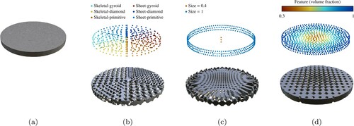
In this paper, we present ASLI (A Simple Lattice Infiller), a cross-platform tool that allows users to provide 3D objects with a functionally graded lattice infill (see Figure 1). The generated functionally graded infills can be hybrid, pseudo-periodic and heterogeneous. The resulting structure is provided to the user in the form of an STL file suitable for 3D printing purposes. If needed, it is also possible to generate volume meshes that can be used for computer simulations.

Figure 1. ASLI can assign functionally graded lattice infills to randomly shaped 3D objects.

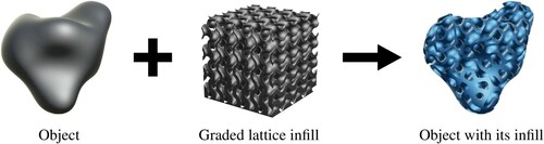
Although developed due to a need to design functionally graded scaffolds for STE applications, ASLI is not application-specific and can therefore be used for any application that requires generating lattice infills. Moreover, even though we have limited ourselves to the implementation of TPMS-based infills, ASLI itself does not have this limitation.

2. Materials and methods

ASLI generates functionally graded scaffold designs following the workflow shown in Figure 2. The process starts by loading the user-provided inputs. Details concerning the user inputs are discussed in Section 2.2. Once the input files are loaded, the preprocessing takes place which, depending on the provided inputs, can include the filtering of data and the construction of linear Radial Basis Function (RBF) interpolation models. Specifics regarding the filtering are found in Section 2.1.1, while the interested reader is referred to Buhmann (2004) for detailed background information on RBF interpolation. The preprocessing is followed by the discretisation step, i.e. the step where the object with its infill is converted into a surface triangulation or volume mesh. The discretisation is performed using the Mmg library (Dapogny et al. 2020) or the Computational Geometry Algorithms Library (CGAL) (CGAL Project 2020). As a result, the user can choose between two workflows in ASLI, the Mmg workflow and the CGAL workflow. The discretised surface is automatically saved as an STL or MESH file, depending on whether it is a surface triangulation or volume mesh.

Figure 2. Schematic representation of the ASLI workflow. Users can provide the inputs either by modifying the configuration file or making use of the graphical user interface. Moreover, they can chose between two different workflows, the Mmg workflow and the CGAL workflow, each with its own advantages and disadvantages.

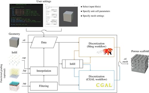
Regardless of the workflow, ASLI uses level-set equations to describe the lattice infill. Their implementation in ASLI is discussed in detail in Section 2.1. A level-set equation provides an implicit description of the infill. In three dimensions, the level-set function ψ will describe an isosurface through an equality of the form $\psi (x,y,z)=l$, where x, y and z are the coordinates of a point in space and l is the isovalue. Isosurfaces are the three-dimensional equivalent of contour lines, while the isovalue is the parameter that determines the isosurface being considered. To provide arbitrary geometries of their infill, the Mmg workflow first generates a volume mesh of the external geometry using the TetGen library (Si 2015). Subsequently, the infill of the geometry is determined by computing the isovalues at the nodes of this volume mesh before the discretisation of the object with its infill starts. The main drawback of this approach is that this mesh needs to be fine enough to capture all features of the level-set. As will be seen in Section 3.1, this means that discretising times will increase exponentially with decreasing feature sizes. The CGAL workflow, on the other hand, uses the Poisson Surface reconstruction method (Kazhdan, Bolitho, and Hoppe 2006) to first compute an implicit function of the geometry that is to be provided with an infill. The infill ${\psi }_{infill}$ is then inscribed to this implicitly described geometry ${\psi }_{geometry}$ by computing the Boolean intersection of them (Yoo 2011). (1) ${\psi }_{geometry}\cap {\psi }_{infill}=min({\psi }_{geometry},{\psi }_{infill})$(1) The implicit surface resulting from this Boolean intersection is then discretised by evaluating the implicit function during the discretisation process. As a result, the time required to evaluate the implicit function has a direct impact on the total discretising time. In ASLI, this can be very detrimental when discretising hybrid, pseudo-periodic or heterogeneous designs with the CGAL workflow, as will be discussed in Section 3.1.

2.1. Unit cells

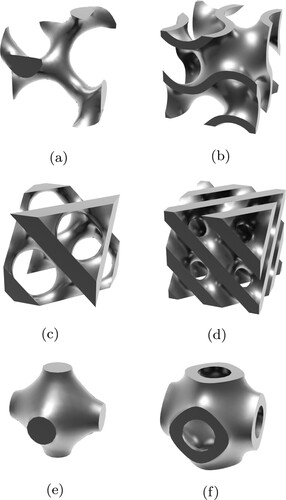
Developed with STE applications in mind, ASLI has a few TPMS-based unit cells commonly used in the field already implemented, i.e. the skeletal and sheet variants of the Gyroid (G), Diamond (D) and Primitive (P) unit cells. An example of each is shown in Figure 3. To describe these TPMS-based unit cells in ASLI, the level-set approximations given by Wohlgemuth et al. (2001) are used. (2) ${\psi }_G\left(\overrightarrow{x}\right)=\sin k_1{x}_1\cos k_2{x}_2+\sin k_2{x}_2\cos k_3{x}_3+\sin k_3{x}_3\cos k_1{x}_1-l$(2) (3) $\begin{array}{rl}{\psi }_D\left(\overrightarrow{x}\right)& =\sin k_1{x}_1\sin k_2{x}_2\sin k_3{x}_3\\ +\sin k_1{x}_1\cos k_2{x}_2\cos k_3{x}_3\\ & +\cos k_1{x}_1\sin k_2{x}_2\cos k_3{x}_3\\ & +\cos k_1{x}_1\cos k_2{x}_2\sin k_3{x}_3-l\end{array}$(3) (4) ${\psi }_P\left(\overrightarrow{x}\right)=\cos k_1{x}_1+\cos k_2{x}_2+\cos k_3{x}_3-l$(4)

In these equations, $\overrightarrow{x}$ is a vector containing the x, y and z coordinate, l is the isovalue, and k is the scaling given by $k_i=2\pi /s_i$ where s is the unit cell size. We have chosen to take $s_1=s_2=s_3$ such that unit cells are always scaled uniformly.

Figure 3. ASLI has six different unit cells already implemented, i.e. the (a) skeletal-gyroid, (b) sheet-gyroid, (c) skeletal-diamond, (d) sheet-diamond, (e) skeletal-primitive and (f) sheet-primitive.

In ASLI, it is possible to specify the unit cell type, size and isovalue¹. Since the isovalue is not an ideal parameter from a designers point of view, there is also the possibility to instead specify the isovalue related parameter of volume fraction $V_{frac}$, wall size $t_{wall}$ or pore size $d_{pore}$. The equations relating these parameters to the isovalue were determined empirically. The approach followed and the equations implemented can be found in Appendix 1. From this point onward, the isovalue and isovalue-related parameters will collectively be referred to as the feature value $v_{feature}$.

While the level-set equations presented above can describe the lattice infill, the infill described is a uniform infill. To introduce unit cell size and feature values that vary throughout the volume, these parameters were simply made dependent on $\overrightarrow{x}$, i.e. $s\left(\overrightarrow{x}\right)$ and $v_{feature}\left(\overrightarrow{x}\right)$. Variation in unit cell type throughout the volume, although a little more involved, can also be achieved. The approach taken to introduce it in ASLI is described in Section 2.1.1.

2.1.1. Unit cell type grading

Designs with more than one unit cell type can be described by considering the weighted sum of the level-set functions in the design (Yang et al. 2014). (5) ${\psi }_{hybrid}\left(\overrightarrow{x}\right)=\sum _{j=1}^n{w}_j\left(\overrightarrow{x}\right)\cdot {\psi }_j\left(\overrightarrow{x}\right)$(5) Here, n is the number of different unit cell types in the design and w is a weight such that  w =1 in the region of unit cell type j, i.e. $R_j$, and 0 otherwise. (6) $w_j\left(\overrightarrow{x}\right)=\{\begin{array}{cc}1& \overrightarrow{x}\in R_j\\ 0& \overrightarrow{x}\notin R_j\end{array}$(6) While such a weighted sum allows to introduce any number of unit cell types in the design, the use of binary weights causes abrupt changes that can lead to discontinuities between regions. A grading strategy, also called hybridisation, can be employed to avoid these abrupt changes. This strategy allows the unit cells to gradually morph from one type to the next by temporarily becoming a hybrid of the unit cells in its surroundings. Although different strategies have already been proposed to this end (Yang et al. 2014; Yoo and Kim 2015; Yang et al. 2017), a slightly different approach is used in ASLI. We use a Gaussian function φ to filter the weights in the neighbourhood $N_p$ of point $\overrightarrow{x}$. (7) $\begin{array}{rl}& w_j^{\ast }(\mathbf{x},\overrightarrow{x})=\frac{\underset{{\displaystyle \sum _{k\in N_p}}}{\phi }\left(\Vert {\mathbf{x}}_k-\overrightarrow{x}\Vert \right)\cdot w_j\left({\mathbf{x}}_k\right)}{\underset{{\displaystyle \sum _{k\in N_p}}}{\phi }\left(\Vert {\mathbf{x}}_k-\overrightarrow{x}\Vert \right)}\\ & \mathrm{w}\mathrm{i}\mathrm{t}\mathrm{h}:\\ & N_p=k\mid \Vert {\mathbf{x}}_k-\overrightarrow{x}\Vert \le r\\ & \phi \left(x\right)=e^{-{\left(\frac{2x}{r}\right)}^2}\end{array}$(7) where r controls the filter radius and $\mathbf{x}$ is a matrix containing the points in the transition region. Filtering the weights with a Gaussian function constitutes a simple mechanism to create a gradual transition and provide direct control over the size of the filtered region. However, as Maskery et al. (2018) called to attention, hybrid unit cells can suffer from a thinning effect that can lead to weakened or disconnected regions. As they proposed, a correction c is used to compensate for this. In ASLI, this correction is applied to the feature value. We base this correction on a user defined correction factor $c_{factor}$ and the filtered weights $w^{\ast }$. (8) $\begin{array}{r}{v}_{feature,j}^{\ast }(\mathbf{x},\overrightarrow{x})=c_j(\mathbf{x},\overrightarrow{x})\cdot v_{feature}\left(\overrightarrow{x}\right)\\ & \mathrm{w}\mathrm{i}\mathrm{t}\mathrm{h}:\\ & c_j(\mathbf{x},\overrightarrow{x})=1+c_{factor}\cdot (1-{(2\frac{w_j^{\ast }(\mathbf{x},\overrightarrow{x})}{\Vert {\overrightarrow{w}}^{\ast }(\mathbf{x},\overrightarrow{x})\Vert }-1)}^2)\end{array}$(8) By using the filtered weights, we ensure both that the correction taking place is limited to the transition region, and that the correction will be largest at the centre of the transition region while gradually decreasing to zero as it approaches the transition boundary. The correction factor to be provided is a scalar value equal to or larger than zero. The higher the correction factor, the stronger the correction that will take place.

By considering the filtered weights and the corrected feature value, a corrected level-set function ${\psi }^{\ast }$ can be obtained that provides a smooth continuous transition. (9) ${\psi }_{hyb}^{\ast }(\mathbf{x},\overrightarrow{x})=\sum _{j=1}^n\frac{w_j^{\ast }(\mathbf{x},\overrightarrow{x})}{\Vert {\overrightarrow{w}}^{\ast }(\mathbf{x},\overrightarrow{x})\Vert }\cdot {\psi }_j^{\ast }(\mathbf{x},\overrightarrow{x})$(9) Note that the filtered weights in Equations (8(8) $\begin{array}{r}{v}_{feature,j}^{\ast }(\mathbf{x},\overrightarrow{x})=c_j(\mathbf{x},\overrightarrow{x})\cdot v_{feature}\left(\overrightarrow{x}\right)\\ & \mathrm{w}\mathrm{i}\mathrm{t}\mathrm{h}:\\ & c_j(\mathbf{x},\overrightarrow{x})=1+c_{factor}\cdot (1-{(2\frac{w_j^{\ast }(\mathbf{x},\overrightarrow{x})}{\Vert {\overrightarrow{w}}^{\ast }(\mathbf{x},\overrightarrow{x})\Vert }-1)}^2)\end{array}$(8) ) and (9(9) ${\psi }_{hyb}^{\ast }(\mathbf{x},\overrightarrow{x})=\sum _{j=1}^n\frac{w_j^{\ast }(\mathbf{x},\overrightarrow{x})}{\Vert {\overrightarrow{w}}^{\ast }(\mathbf{x},\overrightarrow{x})\Vert }\cdot {\psi }_j^{\ast }(\mathbf{x},\overrightarrow{x})$(9) ) are normalised to ensure the sum of the weight vector components remains 1.

2.2. Using ASLI

ASLI requires users to specify the STL file containing the object that is to be provided with an infill. The STL file should contain a watertight closed surface. In addition, users have to specify some settings and parameters. This can be done by directly modifying the configuration file located by default in the main folder. Alternatively, users can make use of the Graphical User Interface (GUI) of ASLI shown in Figure 4 to provide the input settings.

Figure 4. Graphical user interface of ASLI: (a) main interface with the lattice tab visible, (b) mesh tab and (c) run tab.

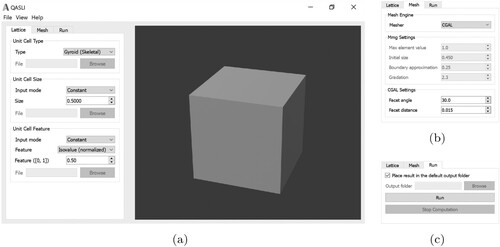
Users can specify the type, size and feature parameters of the unit cells as well as the meshing parameters. The unit cell parameters can be varied over the volume by providing local specifications for the unit cell type, size and feature. This is achieved by additionally supplying the respective TAP (type at points), SAP (size at points), and FAP (feature at points) files. These are comma-delimited files, with 4 columns per row. The first 3 columns of each row correspond to the x, y and z coordinates of the point for which the local scaffold specification is provided in the corresponding 4th column. The local specifications should be given on a set of discrete points, whose convex hull covers the domain of the geometry to be provided with an infill. Figure 5 shows three examples where the type, size and feature have been specified using a set of discrete points.

Figure 5. ASLI can generate hybrid, pseudo-periodic and heterogeneous infills by specifying the unit cell type, size and feature at different points throughout the volume: (a) input STL geometry, (b) specified types with resulting hybrid lattice, (c) specified sizes with resulting pseudo-periodic lattice, and (d) specified feature values with resulting heterogeneous lattice.

Although interpolation models are constructed to efficiently compute intermediate values when type, size and feature values are specified using data points, it is strongly advised that the density of the provided data points is not more than strictly necessary. This is particularly important when using the CGAL workflow, as a large number of data points will lead to significant slowdowns during discretisation. This is further discussed in Section 3.1. Users should also take into consideration that if multiple scaffold types are assigned, the density of the data points specifying unit cell type in transition regions should be such that they can adequately capture the effect of the filter (see Section 2.1.1). When variable sizes or feature values are specified, very large non-smooth variations over small distances, compared to the local unit cell size, should be avoided to avoid unconnected unit cells or other unexpected behaviours. It should also be taken into account that changes in size cannot be decoupled from unit cell deformations. Deformations that may arise due to variable unit cell sizes can be seen in Figure 5(c).

Meshing parameters provided by the user are relative to unit cell sizes or features. This is done not only to have more intuitive input parameters, but also to ensure the resulting surface triangulation captures the infill with similar accuracy regardless of local unit cell size, and that in volume meshes the cross section of unit cell walls discretises with approximately equal number of elements regardless of local wall sizes. Arguably the most important mesh parameter in both workflows is the one controlling how well the surface is approximated. In the CGAL workflow, this is determined by the facet distance while in the MMG workflow by the Hausdorff value. In addition to the aforementioned parameter both workflows have a number of optional settings that allow the user to further control the properties of the output mesh.

The cube that is provided with an infill in the workflow shown in Figure 2 is available in ASLI's repository as a sample problem. The infill is uniform by default and can be set to be hybrid, pseudo-periodic, heterogeneous, or a combination thereof, by using the TAP, SAP and FAP files also available. Step by step instructions on how to run the demo are given in the User Manual found in the Supplementary Materials Section.

2.2.1. Compiling the code

While the easiest way to get started with ASLI is to use its pre-build binaries, available for both Linux and Windows in ASLI's repository, more advanced users may prefer to build ASLI on their computers as this is not only likely to increase performance but will also enable them to customise ASLI according to their needs.

Compiling ASLI is fairly simple and straightforward. Assuming CGAL's dependencies GMP (see gmplib.org), MPFR (see www.mpfr.org), Boost (see www.boost.org) and oneTBB² (see github.com/intel/tbb) as well as the GUI dependency QT³ (see www.qt.io) have already been installed on the system, this will only require the following steps on a 64-bit Linux platform.

(1)	Download the code from github.com/tpms-lattice/ASLI and extract
(2)	Type in the terminal the following sequence of commands  $ mkdir build  $ cd build  $ cmake -DCMAKE_BUILD_TYPE=Release -DMARCH_NATIVE=ON -DASLI_GUI=ON ..  $ make  $ cd ../bin
(3)	Type ./ASLI config.yml to run the code.
(4)	Visualise the output file(s).4

Fully detailed compilation instructions for Linux as well as Windows can be found in the User Manual provided in the Supplementary Material Section.

2.2.2. Extending the code

The code has been divided into the clearly separated units detailed below.

• ASLI: class containing all the relevant parameters and general settings.

• Infill: namespace containing all equations related to the lattice infill.

• Filter: namespace containing the weight filter.

• TrilinearInterpolation: namespace containing an implementation of an RBF interpolation with linear kernel.

• MeshMMG: namespace containing the Mmg API calls required to discretise the infill.

• MeshCGAL: namespace containing the CGAL API calls required to discretise the infill.

Organising the code in this way allows users to easily adapt the code to suit their needs. For example, to include new unit cells, the user only has to add a few equations to the code. These would be the equation describing the new unit cell, as well as the corresponding equations relating the isovalue to the wall and pore size, and the equations relating volume fraction, wall size and pore size to the isovalue. These are to be added to the appropriately named functions found in the Infill namespace: TPMS_function, isovalue2wallSize, isovalue2poreSize, vFraction2isovalue, wallSize2isovalue and poreSize2isovalue.

Other changes, like introducing new feature parameters, modifying the filter or introducing non-uniformly scaled unit cells, can be accomplished by modifying the relevant namespaces, and at times, also the ASLI class. More involved changes, like introducing a new library to discretise the implicit function, can best be accomplished by writing a new namespace.

3. Results and discussion

To ascertain how the performance of ASLI's workflows compare, as well as to better understand their strengths and weaknesses, a benchmarking was performed whose results are shown and discussed in Section 3.1. In Section 3.2, the performance of ASLI and similar freeware and free-and-open-source tools is compared. Finally, the capabilities of ASLI are showcased in Section 3.3 through a series of examples. In the first two examples, an acetabular shell and a femoral implant were each provided with a lattice infill according to different specifications to afterwards be 3D printed, while in the third example a cylinder was provided with an infill to later be used in Finite Element (FE) simulations.

3.1. Performance

Benchmarking was performed on a Linux 64-bit system equipped with an Intel® Core^TM i7-8850H 6 core CPU and 32 GB of RAM. Performance was assessed by measuring discretising times and utilised RAM, while varying the number of unit cells in a unit cube. The unit cell was given a uniform skeletal-gyroid infill and meshing parameters were kept fixed. The unit cube was considered for infills consisting of one single unit cell, up to a thousand, with a normalised isovalue of 0.5. Given that different meshing parameters are used in the Mmg and CGAL workflows, they have been chosen such that discretisation was performed with approximately similar accuracy. In the Mmg workflow, the Hausdorff value was set to 0.42, while in the CGAL workflow facet distance was set to 0.012. All other mesh settings were used with their default values. The program was compiled in release mode, with MARCH_NATIVE enabled, using GCC v8.3.

The CGAL workflow was found to be the faster of the two workflows, as shown by Figure 6(a), when no use was made of data points to specify unit cell type, size or feature. For a lower number of unit cells the difference in discretisation times was limited, but for a larger number of unit cells the difference became significant. Benchmarkings suggest discretisation times of the CGAL workflow increase linearly while the discretisation times of the Mmg workflow increase exponentially, with increasing number of unit cells (decreasing feature sizes). The striking difference in performance, especially for a larger number of unit cells, is the result of the different approaches to discretisation taken by the Mmg and CGAL libraries. In the case of Mmg, nodal implicit function values are required to capture the level-set. Therefore, we need a certain node density not to undersample as we might otherwise miss infill features. This means that as relative feature sizes decrease, the number of nodal points required to capture all features will increase exponentially, which leads to the observed exponential increase in discretisation times. CGAL does not rely on nodal values to capture the level-set, instead it constantly evaluates the implicit function during discretisation. As can be seen, this clearly provides an advantage during the discretisation of structures with a uniform infill. However, as shown by Figure 6(b), this can be a disadvantage during the discretisation of structures with a hybrid, pseudo-periodic or heterogeneous infill.

Figure 6. The performance of ASLI as determined with a skeletal-gyroid: (a) meshing times, (b) interpolation slowdown, (c) memory consumption and (d) parallel speed-up.

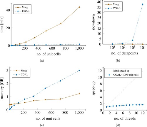
When dealing with hybrid, pseudo-periodic or heterogeneous infills the user is required to specify parameters on a set of points throughout the volume, see Section 2.2. Subsequently, interpolation models are constructed for each parameter varying throughout the volume. The time required to evaluate these interpolation models increases with an increasing number of data points, which in turn increases the evaluation time of the implicit function. The slowdowns that can be observed in Figure 6(b) are a direct consequence of this. We can see the CGAL workflow suffers from an exponentially increasing slowdown when increasing number of data points are used to specify the infill. Not using more data points than strictly necessary to specify the varying unit cell properties is therefore advisable when using the CGAL workflow. The Mmg workflow, in contrast, experiences a negligible slowdown with increasing number of data points. This is because precomputed nodal implicit function values are used, meaning the implicit function is evaluated before and not while discretising.

A preferred workflow from a RAM requirements point of view is more difficult to ascertain. As seen in Figure 6(c), up to about two hundred unit cells, memory requirements were found to be lower for the CGAL workflow. For a higher number of unit cells, the Mmg workflow proved to have lower memory requirements. However, measurements seem to indicate that memory requirements scale linearly for the CGAL workflow and superlinearly for the Mmg workflow. If this trend sets forth, the memory requirements of the Mmg workflow will eventually overtake again those of the CGAL workflow, and therefore, for a larger number of unit cells (smaller feature sizes), the CGAL workflow should again become the preferred one from a memory point of view.

ASLI can also operate in parallel mode. This is, however, limited to the CGAL workflow because the parallel version of Mmg (Cirrottola and Froehly 2019) is, at the time of writing, not yet capable of discretising implicit functions. The decrease in discretising times measured for the CGAL workflow when making use of parallelisation was found to be marginal at best, as can be seen in Figure 6(d). Speed-up was about 1.45 with 6 threads after which further improvement was found to be negligible. We expect this can be improved in the future with some code optimisation on the side of ASLI.

It should be emphasised that this analysis is intended to give some insight into the advantages and disadvantages of each workflow, with the goal of placing the user in a better position when it comes to making a choice on the workflow to use. It was not, in any way, intended to determine approximate meshing times or resource requirements, as these are extremely dependent on the unit cell type, its minimal feature size, the mesh settings, and computational resources available, among others.

3.2. Performance compared to other tools

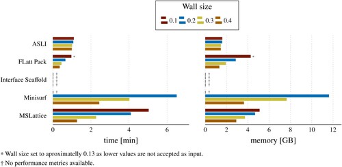
To carry out the performance comparison we retrieved the freeware and free-and-open-source tools with similar functionality to ASLI known to us from their repositories and tested them, i.e. we retrieved FLatt Pack (Maskery et al. 2022), Interface Scaffold (Dinis et al. 2014), Minisurf (Hsieh and Valdevit 2020) and MSLattice (Al-Ketan and Abu Al-Rub 2020). The comparison was carried out in Windows as it is the only operating system on which all tools are supported. A 64-bit laptop equipped with an Intel® Core^TM i7-8665U 4 core CPU, 16 GB RAM and running Windows 10 was used. To determine performance, unit cubes were assigned the same infills with each of the tools being considered, while peak RAM usage and the time it took to discretise and store the generated infills as STL files was recorded. In total, four different uniform infills were used to assess performance. All infills were comprised of 1000 skeletal-gyroid unit cells, and differed only in volume fraction. Volume fractions of 0.731e−1, 0.165, 0.303 and 0.473 were prescribed leading to wall sizes of approximately 0.1, 0.2, 0.3 and 0.4. As we consider wall sizes relative to the unit cell size they are dimensionless. We will focus on wall sizes for this comparison as they represent the size of the smallest feature of these infills which, if using a grid as most of the tools considered do, is ultimately what determines the size of the grid required to successfully capture all features of the infill and thus the time it will take to discretise.

Since FLatt Pack does not give users control over the discretisation accuracy or the density of the grid used to compute the infills, the grid densities it selects have to be used. In our case, these were 33, 25 and 20 for the infills with wall sizes of 0.2, 0.3 and 0.4, respectively. It was not possible to create a lattice with wall sizes of 0.1 because Flatt Pack has a lower limit of 10% on the volume fractions of skeletal-gyroids. Therefore, with FLatt Pack, we instead constructed a lattice at the lowest possible volume fraction allowed which translates to a wall size of approximately 0.13. To keep parameters as similar as possible across the different tools, we used the same grid densities used by FLatt Pack when constructing the lattices with MSLattice and Minisurf.⁵ As there was no value dictated by FLatt Pack for the infill with a wall size of 0.1, we considered the observed exponential decrease in grid density with decreasing volume fraction to determine a grid density of 45. Deciding on the input settings for ASLI was less straightforward as it does not make use of an underlying grid like the other tools, and inversely, none of the other tools provide an approximation error. Thus, we opted to run ASLI with its default settings. This means the CGAL workflow was used, no use was made of parallel resources and the approximation error of the final triangulation was 0.015 times the unit cell size. The Mmg workflow of ASLI was not considered in this comparison as its main function is creating quality tetrahedral meshes, a capability not shared by any of the other tools. Interface Scaffold was not tested because, at present, it cannot create skeletal-gyroid infills.

Although the fastest discretisation times achieved were with FLatt Pack, followed by ASLI as can be seen in Figure 7, FLatt Pack discretisation times were found to almost triple as wall sizes grew smaller, while ASLI's times remained nearly identical. As a result, the difference in the time required by FLatt Pack and ASLI to create the infills reduced to the point of being nearly identical at the smallest wall size considered. Under normal use scenarios, ASLI's times are expected to decrease compared to those measured here, as parallel capabilities would normally be used. MSLattice and Minisurf were the slowest tools and, like FLatt Pack, the time required to create the lattices increased significantly as wall sizes decreased. A similar trend was observed when looking at peak memory usage. All tools, except ASLI, had a noticeable increase in memory consumption with decreasing wall size. Considering actual memory footprint, ASLI was found to have the overall lowest one, followed by FLatt Pack whose memory use ranged from similar to ASLI's to about two and a half times as high. MSLattice was found to use a little more memory than FLatt Pack, while Minisurf proved to be particularly memory intensive as made clear by the fact that our system had to start memory paging while generating the infill with a wall size of 0.1, which is the reason this measurement was excluded from the results.

Figure 7. Performance comparison between the different freeware and free-and-open-source tools as determined with a skeletal-gyroid.

It should be highlighted that this comparison is only intended to give a sense of how the different tools perform. A thorough comparison would require the consideration of many more scenarios. Moreover, it would ideally take place between solutions with the same approximation errors, as this would be the most meaningful.

3.3. Examples

In the following, three examples are presented that showcase ASLI's capabilities to generate functionally graded designs for real-world applications. The examples were generated using 6 threads on a 64-bit laptop equipped with an Intel® Core^TM i7-8665U 4 core CPU and 16 GB RAM. The laptop was running Windows 10.

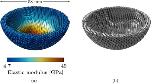
As first example, depicted in Figure 8, a porous acetabular shell was generated by varying the volume fraction of skeletal-gyroids with an unit cell size of 1.5 mm, based on an a priori computed optimised stiffness distribution (see Figure 8(a)). Roughly 1200 data points were used to specify the volume fraction. The porous shell was discretised using the CGAL workflow with default meshing parameters and a facet distance of 0.015. It took approximately 45 min to discretise and the resulting surface triangulation, shown in Figure 8(a), comprised 2,635,420 vertices and 5,347,924 faces. The generated structure was manufactured by 3D Systems (3D Systems, Leuven, Belgium) in Ti6Al4V ELI (grade 23), see Figure 8(b), through direct metal laser sintering using a DMP Flex 350 machine.

Figure 8. The shell of an acetabular implant was assigned a skeletal-gyroid infill of varying volume fraction to match a desired stiffness distribution: (a) ASLI generated 3D-model overlaid with the material stiffness distribution (b) additively manufactured acetabular shell.

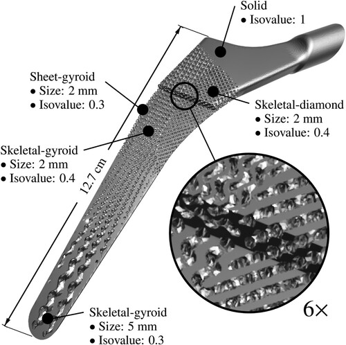
In the second example, the stem of a femoral implant was provided with the hybrid pseudo-periodic heterogeneous infill shown in Figure 9. Skeletal-gyroid, sheet-gyroid and skeletal-diamond unit cells were used with sizes ranging from 2 to 5 mm and normalised isovalues between 0.3 and 1. The unit cell type, size and feature were specified using around 6000, 200 and 1500 data points, respectively. Discretisation was performed with the CGAL workflow and took approximately 56 min. Default meshing parameters were used and facet distance was set to 0.022. The final triangulated surface was comprised of 2,074,203 vertices and 4,165,514 faces.

Figure 9. ASLI generated 3D-model of a femoral implant with a graded lattice where unit cell type, size and isovalue are varied. The top half of the lower section of the implant has been hidden to also show the internal structure. The transition between three different lattice types can be seen to happen smoothly in the close-up.

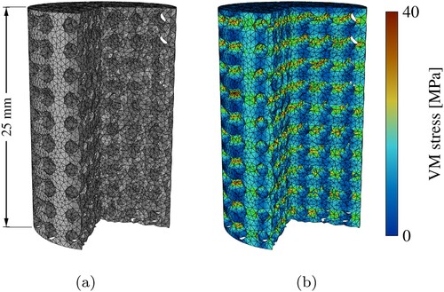
As the third and final example, a $16\times 25$ porous titanium cylinder, commonly used to experimentally determine material properties of STE scaffolds, was discretised to use in a FE simulation. The cylinder was provided with a skeletal-primitive infill constructed out of unit cells of 2.5 mm with a volume fraction of 0.45. The Mmg workflow was used to discretise the cylinder with the Hausdorff value set to 0.2. Additionally, the optional meshing parameters of minimum and maximum mesh edge length where set to 0.2 and 0.3, respectively. All other meshing parameters were kept at their default values. Discretisation took approximately 15 min and the generated volume mesh, shown in Figure 10(a), consisted of 45,564 vertices and 167,319 tetrahedra. The generated mesh was subsequently used to perform a FE analysis in Abaqus/CAE 2017 (Dassault Systèmes Simulia Corp., Johnston, RI, USA). Z-symmetric boundary conditions were applied at the bottom of the cylinder and a distributed compression load of 1 kN was applied at the top simulating a standard unconfined compression test. The material was assumed to be elastic isotropic with Young's modulus of 110 GPa and a Poisson ratio of 0.3. The computed von Mises stresses are depicted in Figure 10(b).

Figure 10. Volume meshes generated by ASLI can be used in finite element simulations: (a) volume mesh of a cylinder provided with a skeleton-primitive infill and (b) FE simulation result. One quarter of the cylinder has been hidden to show internal structure and stresses.

These examples show ASLI is capable of generating manufacturable functionally graded lattice structures for real-world applications as well as for FE simulations. The lattice structures can be hybrid, pseudo-periodic, heterogeneous or a combination hereof. Moreover, there is no limitation when it comes to the shape of the object that is to be provided with an infill.

4. Concluding remarks

ASLI is a cross-platform open-source tool capable of creating functionally graded lattice infills with minimal effort. Freeware and free-and-open-source tools of similar functionality, although available, are often limited to cuboid shapes with at most the option to specify different uniform volume fractions (Dinis et al. 2014; Hsieh and Valdevit 2020). MSLattice (Al-Ketan and Abu Al-Rub 2020), a more advanced tool, allows users to create lattices of varying unit cell types with size and volume fraction grading. However, the mechanism employed to specify multiple unit cell types and grading is not ideal, as it requires users to provide this information in equation form, which is cumbersome even for the simplest of cases. Furthermore, although not limited to cuboid shapes, it is still limited to just a few built-in geometries. More recently, FLatt Pack (Maskery et al. 2022) was released which improves on this limitation by making it possible for users to assign infills with volume fraction grading to arbitrary shapes. Unfortunately, it does not support multiple unit cell types in a design nor a varying unit cell size. Additionally, although it is capable of generating volume meshes unlike the previous tools, this is limited to voxel meshes, which restricts the types of analyses that can be performed with them. In ASLI we have brought together features currently scattered between different freeware and free-and-open-source tools and further improved upon them. As a result, users can assign infills of varying unit cell type, size and feature, including volume fraction, to arbitrary shapes and subsequently generate surface triangulations and tetrahedral volume meshes. We have also made an effort to keep the method used to provide gradation data as simple and straightforward as possible, effectively making it easier for users to define complex functionally graded designs. This was achieved by requesting users to specify the local type, size or feature values on a discrete set of points. In addition, to ensure optimal mesh sizes throughout, mesh sizes have been coupled to unit cell size and feature values, which has the added benefit of minimising required resources. In other words, with ASLI it is possible to create functionally graded scaffolds with more flexibility and at larger scales than was possible with previously available freeware and free-and-open-source tools.

Besides freeware and free-and-open-source tools, there are also some commercial tools available that offer the functionality of generating TPMS-based lattices. Generally speaking, these are more capable but tend to be expensive and often require active user intervention, which makes them less suitable for automatic workflows. Compared to commercial tools, ASLI's main advantage, besides its free availability and the possibility to make changes to its source code, is that it was created to be used in a workflow with minimal to no user intervention where the functional grading is determined automatically based on the results of computational analysis. As a result, it is possible to, e.g. couple it to an FE simulation or an optimisation routine so that at the end of the analysis ASLI automatically generates a functionally graded infill based on the obtained outputs. An overview of the features offered by the different tools just discussed is found in Table 1.

Table 1. Overview of tools (Maskery et al. 2022; Dinis et al. 2014; Hsieh and Valdevit 2020; Al-Ketan and Abu Al-Rub 2020; NTopology 2021; McNeel et al. 2021; Synopsys 2021) for the generation of TPMS-based lattices.

	User defined 3D geometry	Uniform infill	Hybrid infill	Pseudo-periodic infill	Heterogeneous infill	Conformal infill	Parallelised operations	Graphical user interface	Automation friendly	Creates surface triangulations	Creates volume meshes	Windows support	Linux support	macOS support	Freely available (open-source)
ASLI	✓	✓	✓	✓	✓	·	✓^1	✓	✓	✓	✓	✓	✓	·	✓(✓)
FLatt Pack	✓	✓	·	·	✓	·	·	✓	·	✓	✓^2	✓	·	·	✓(✕)
Interface Scaffold	·	✓	·	·	·	·	·	✓	·	✓	·	✓	✓	·	✓(✓)
Minisurf	·	✓	·	·	·	·	·	✓	·	✓^3	·	✓	·	·	✓(✓)
MSLattice	·	✓	✓	✓	✓	·	·	✓	·	✓	·	✓	✓	·	✓(✕)
NTopology	✓	✓	✓	✓	✓	✓	✓	✓	·	✓	✓	✓	·	·	·
Rhino 3D (with plugins)	✓	✓	✓	✓	✓	✓	·	✓	·	✓	✓	✓	·	✓	·
ScanIP+CAD	✓	✓	✓^4	✓^4	✓^4	·	✓	✓	·	✓	✓	✓	✓	·	·

${}^1$Limited to the CGAL workflow.${}^2$Tetrahedral meshing is not supported.${}^3$Surfaces generated have no wall thickness.${}^4$Continuously graded infills are not supported.

Despite its strengths, like every other tool, ASLI also has its limitations. At present, ASLI cannot process more than one object at a time nor create conformal infills. Specific to the CGAL workflow, ASLI tends to fail at detecting and discretising small closed regions and is not yet capable of preserving sharp edges when creating volume meshes. Finally, parallelisation in ASLI is currently limited to the CGAL workflow and is still suboptimal. Further code optimisation should lead to an improvement in the parallel performance of the CGAL workflow, while the expected future addition of isovalue discretisation to ParMmg will allow to eventually also add parallel capabilities to the Mmg workflow.

As ASLI matures, we expect to improve on its current limitations. In the meantime, we believe that its current capabilities will already prove useful across a wide range of fields, especially given the increasing interest in TPMS-based functionally graded materials, not only in the field of STE, but also for applications ranging from energy-absorbing structures (Maskery et al. 2017; Zhang et al. 2018) to heat transfer modules (Catchpole-Smith et al. 2019; Femmer, Kuehne, and Wessling 2015; Li, Yu, and Yu 2020) and light-weight fuel cells (Han et al. 2017).

Disclosure statement

No potential conflict of interest was reported by the author(s).

Additional information

Funding

This work was supported by the European Regional Development Fund – Interreg VA Flanders - The Netherlands (PRosPERoS, CCI 2014TC16RFCB046); the European Union's Horizon 2020 Research and Innovation Programme via the European Research Council (ERC CoG INSITE 772418); the Fund for Scientific Research Flanders (G085018N); the Fédération Wallonie-Bruxelles through the BioWin project BIOPTOS (7560); and the KU Leuven Special Research Fund (C24/17/07).

Notes on contributors

Fernando Perez-Boerema

Fernando Perez-Boerema is a PhD candidate at the Biomechanics Section of the KU Leuven in Belgium.

Mojtaba Barzegari

Mojtaba Barzegari is a PhD candidate at the Biomechanics Section of the KU Leuven in Belgium.

Liesbet Geris

Liesbet Geris is a Full Professor in Biomechanics and Computational Tissue Engineering at the University of Liège and KU Leuven in Belgium.

Notes

1 If the isovalue is given as input, it must be provided as a min-max normalised isovalue.

2 OneTBB is only required if ASLI is compiled for parallel use. To compile ASLI with parallel support add -DCGAL_ACTIVATE_CONCURRENT_MESH_3=ON to the cmake call.

3 QT is only required if the GUI of ASLI is also being compiled.

4 Gmsh (see gmsh.info) can be used to visualize the STL and MESH output files.

5 Minisurf limits the faces in the final triangulation to 30³. As this made it impossible to create the lattices used for the comparison, we changed the source code to instead reduce the number of initial faces by 90%.

Appendix 1.

Feature-isovalue conversions

The volume fraction, wall size and pore size of TPMS-based unit cells are intrinsically dependent on the isovalue. Equations describing these relationships were estimated virtually with an in-house MATLAB (The MathWorks Inc., Natick, MA, USA) code. To this end, a unit cube with a single unit cell, built on a $768\times 768\times 768$ resolution grid, was considered. The resolution was determined by starting with a $3\times 3\times 3$ grid, and doubling the resolution until the discretisation errors of the measured quantities were in the order of ${10}^{-3}$. A skeletal-gyroid unit cell of volume fraction 0.5 is shown in Figure A1 for the intermediate $48\times 48\times 48$ grid.

Figure A1. To estimate the volume fraction, wall size and pore size of the unit cells, their geometry was approximated on an increasingly refined grid until the desired accuracy was reached. The skeletal-gyroid unit cell, with a volume fraction of 0.5, is here shown for the $48\times 48\times 48$ intermediate grid. The solid side skeletal graph and void side skeletal nodes were used to aid in the virtual measurements.

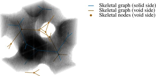
The volume fraction, defined as the solid side volume divided by the total volume, was estimated by taking the number of solid voxels within the unit cube and dividing them by the total number of voxels. To determine the wall thickness, i.e. the solid side minimum thickness, different approaches were used for skeletal and sheet unit cells. The need for different approaches stems from the fact that in skeletal unit cells the triply periodic surface is considered to be the boundary between solid and void, while in sheet unit cells the triply periodic surface is offset to create the solid space. The wall thickness of skeletal unit cells was estimated by first computing the solid side skeleton and, subsequently, determining the minimum distance from the skeleton to the scaffolds surface. The wall thickness of sheet unit cells could directly be determined by computing the minimum solid side distance between its two surfaces. Finally, the pore size of skeletal and sheet unit cells was determined, i.e. the diameter of the largest sphere that can be fitted in the void space of the unit cell. To determine the pore size, first the void side skeleton nodes of the unit cell were located. These nodes indicate the locations of the largest spheres centroids. The diameter of the largest sphere was determined as the minimum distance between the void side skeleton node and the scaffold surface. Distances were determined using a kd-tree nearest neighbour search.

The virtual measurements were taken for the entire isovalue range of skeletal and sheet-gyroid, diamond and primitive unit cells. A total of 43 equally distanced data points were acquired for each unit cell type. The relationships between the measured quantities and the isovalues were determined by fitting polynomials ranging between first and sixth order to the data. (A1) $P\left(x\right)=a+bx+c{x}^2+d{x}^3+e{x}^4+f{x}^5+g{x}^6$(A1) While volume fraction is independent of unit cell size, wall and pore sizes scale linearly with it. Therefore, polynomials fitted to size and feature data are multiplied by the unit cell size in order to make the estimations size independent, i.e. $t_{wall}=s\cdot P\left(x\right)$ and $d_{pore}=s\cdot P\left(x\right)$.

The measured data and polynomial fits are shown in Figure A2 with the corresponding discretisation errors in Fig A3. The polynomial coefficients are given in Table A1.

Figure A2. Virtually measured volume fraction, wall size and pore size for gyroid, diamond and primitive unit cells with corresponding polynomial fits.

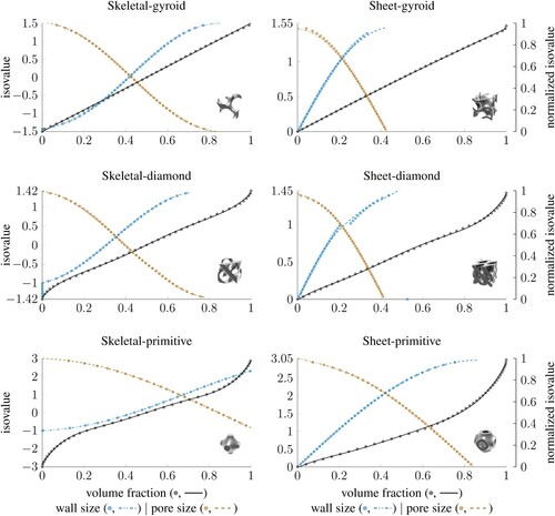
Figure A3. Discretisation errors of virtually measured volume fraction, wall size and pore size for gyroid, diamond and primitive unit cells.

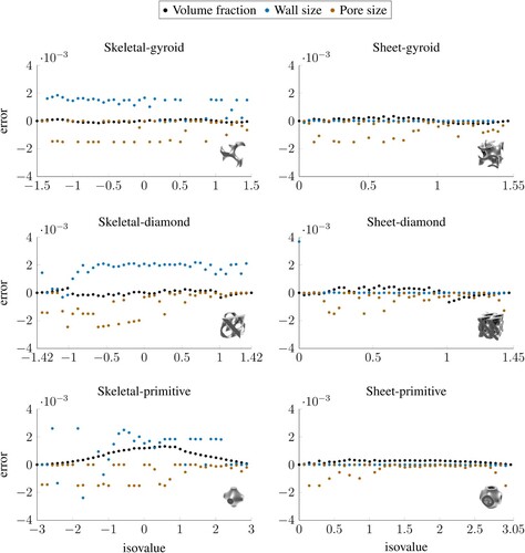
Table A1. Coefficients of the fitted polynomials.

TPMS	Type	Function	Coefficients
			a	b	c	d	e	f
Gyroid	Skeletal	$l\left(V_{frac}\right)$	−1.5	3.0	–	–	–	–
		$l\left(t_{wall}\right)$	−1.43	1.05	2.80	19.83	−37.50	16.70
		$l\left(d_{pore}\right)$	1.52	−0.486	−7.57	−6.28	21.03	−9.61
		$t_{wall}\left(l\right)$	0.415	0.197	−0.00343	−0.0202	−0.00393	0.0273
		$d_{pore}\left(l\right)$	0.428	−0.191	0.00166	0.00822	−0.00133	−0.0169
	Sheet	$l\left(V_{frac}\right)$	−0.00224	1.59	−0.117	−	−	−
		$l\left(t_{wall}\right)$	−0.0350	6.55	−6.99	–	–	–
		$l\left(d_{pore}\right)$	1.47	−0.314	−6.84	−15.23	50.37	−40.61
		$t_{wall}\left(l\right)$	−0.00584	0.387	−1.24	2.73	−2.43	0.767
		$d_{pore}\left(l\right)$	0.432	−0.264	0.418	−0.893	0.782	−0.253
Diamond	Skeletal	$l\left(V_{frac}\right)$	−1.36	5.61	−19.59	49.46	−54.60	21.84
		$l\left(t_{wall}\right)$	−0.984	0.904	10.63	−10.19	−	−
		$l\left(d_{pore}\right)$	1.40	−0.497	−11.42	9.63	−	−
		$t_{wall}\left(l\right)$	0.305	0.222	0.00838	0.00314	−0.0462	0.0470
		$d_{pore}\left(l\right)$	0.395	−0.208	0.0180	0.0144	−0.00916	−0.0251
	Sheet	$l\left(V_{frac}\right)$	−0.0108	1.82	−5.48	17.74	−23.55	10.88
		$l\left(t_{wall}\right)$	−0.0396	7.07	−13.42	10.71	−	−
		$l\left(d_{pore}\right)$	1.41	−1.09	3.81	−65.70	153.92	−119.84
		$t_{wall}\left(l\right)$	−0.00219	0.226	−0.155	0.160	−	−
		$d_{pore}\left(l\right)$	0.421	−0.288	0.568	−1.26	1.16	−0.397
Primitive	Skeletal	$l\left(V_{frac}\right)$	−2.86	18.57	−74.78	170.67	−181.17	72.43
		$l\left(t_{wall}\right)$	−0.999	0.604	3.55	2.18	−4.21	1.19
		$l\left(d_{pore}\right)$	3.00	−0.504	−3.83	−1.56	2.68	−0.619
		$t_{wall}\left(l\right)$	0.442	0.251	−0.0551	0.0690	−0.0370	0.00717
		$d_{pore}\left(l\right)$	0.843	−0.193	0.00123	0.00326	−0.000306	−0.00123
	Sheet	$l\left(V_{frac}\right)$	−0.0250	2.83	−8.89	26.90	−34.93	17.03
		$l\left(t_{wall}\right)$	7.80e−05	5.44	0.0212	−3.07	0.170	0.355
		$l\left(d_{pore}\right)$	3.05	−1.42	1.23	−13.67	15.75	−5.86
		$t_{wall}\left(l\right)$	−0.00488	0.236	−0.140	0.150	−0.0652	0.0106
		$d_{pore}\left(l\right)$	0.847	−0.225	0.113	−0.125	0.0558	−0.00943

References

- Al-Ketan O., and R. K. Abu Al-Rub. 2020. “MSLattice: A Free Software for Generating Uniform and Graded Lattices Based on Triply Periodic Minimal Surfaces.” Material Design & Processing Communications 3 (6): 1–10. doi:https://doi.org/10.1002/mdp2.205.
- Buhmann M. D. 2004. Radial Basis Functions. Cambridge, United Kingdom: Cambridge University Press. doi:https://doi.org/10.1017/CBO9780511543241.
- Catchpole-Smith S., R. R. J. Sélo, A. W. Davis, I. A. Ashcroft, C. J. Tuck, and A. Clare. 2019. “Thermal Conductivity of TPMS Lattice Structures Manufactured Via Laser Powder Bed Fusion.” Additive Manufacturing 30: 100846. doi:https://doi.org/10.1016/j.addma.2019.100846
- Cirrottola L., and A. Froehly. 2019. Parallel unstructured mesh adaptation using iterative remeshing and repartitioning. Research Report RR-9307. INRIA Bordeaux, équipe CARDAMOM. https://hal.inria.fr/hal-02386837.
- Cloutier M., D. Mantovani, and F. Rosei. 2015. “Antibacterial Coatings: Challenges, Perspectives, and Opportunities.” Trends in Biotechnology 33 (11): 637–652. doi:https://doi.org/10.1016/j.tibtech.2015.09.002
- Dapogny C., C. Dobrzynski, P. Frey, and A. Froelhy. 2020. “Mmg platform: Robust, open-source and multidisciplinary software for remeshing.” https://github.com/MmgTools/mmg.
- Dinis J. C., T. F. Morais, P. H. J. Amorim, R. B. Ruben, H. A. Almeida, P. N. Inforçati, P. J. Bártolo, and J. V. L. Silva. 2014. “Open Source Software for the Automatic Design of Scaffold Structures for Tissue Engineering Applications.” Procedia Technology 16: 1542–1547. doi:https://doi.org/10.1016/j.protcy.2014.10.176.
- Femmer T., A. J. C. Kuehne, and M. Wessling. 2015. “Estimation of the Structure Dependent Performance of 3-D Rapid Prototyped Membranes.” Chemical Engineering Journal 273: 438–445. doi:https://doi.org/10.1016/j.cej.2015.03.029
- Gibson L. J., and M. F. Ashby. 1997. Cellular Solids. 2nd ed. Cambridge: Cambridge University Press. doi:https://doi.org/10.1017/CBO9781139878326.
- Gibson L. J., M. F. Ashby, and B. A. Harley. 2010. Cellular Materials in Nature and Medicine. Cambridge: Cambridge University Press.
- Goodman S. B., Z. Yao, M. Keeney, and F. Yang. 2013. “The Future of Biologic Coatings for Orthopaedic Implants.” Biomaterials 34 (13): 3174–3183. doi:https://doi.org/10.1016/j.biomaterials.2013.01.074
- Han S. C., J. M. Choi, G. Liu, and K. Kang. 2017. “A Microscopic Shell Structure with Schwarz's D-surface.” Scientific Reports 7 (1): 13405. doi:https://doi.org/10.1038/s41598-017-13618-3
- Heinl P., L. Müller, C. Körner, R. F. Singer, and F. A. Müller. 2008. “Cellular Ti–6Al–4V Structures with Interconnected Macro Porosity for Bone Implants Fabricated by Selective Electron Beam Melting.” Acta Biomaterialia 4 (5): 1536–1544. doi:https://doi.org/10.1016/j.actbio.2008.03.013
- Hollister S. J 2005. “Porous Scaffold Design for Tissue Engineering.” Nature Materials 4 (7): 518–524. doi:https://doi.org/10.1038/nmat1421
- Hsieh M. T., and L. Valdevit. 2020. “Minisurf – A Minimal Surface Generator for Finite Element Modeling and Additive Manufacturing.” Software Impacts 6: 100026. doi:https://doi.org/10.1016/j.simpa.2020.100026
- Kazhdan M., M. Bolitho, and H. Hoppe. 2006. “Poisson surface reconstruction.” In Proceedings of the Fourth Eurographics Symposium on Geometry Processing, Cagliari, Sardinia, Italy. doi:https://doi.org/10.5555/1281957.1281965.
- Li W., G. Yu, and Z. Yu. 2020. “Bioinspired Heat Exchangers Based on Triply Periodic Minimal Surfaces for Supercritical CO2 Cycles.” Applied Thermal Engineering 179: 115686. doi:https://doi.org/10.1016/j.applthermaleng.2020.115686
- Maskery I., N. T. Aboulkhair, A. O. Aremu, C. J. Tuck, and I. A. Ashcroft. 2017. “Compressive Failure Modes and Energy Absorption in Additively Manufactured Double Gyroid Lattices.” Additive Manufacturing 16: 24–29. doi:https://doi.org/10.1016/j.addma.2017.04.003
- Maskery I., A. O. Aremu, L. Parry, R. D. Wildman, C. J. Tuck, and I. A. Ashcroft. 2018. “Effective Design and Simulation of Surface-based Lattice Structures Featuring Volume Fraction and Cell Type Grading.” Materials & Design 155: 220–232. doi:https://doi.org/10.1016/j.matdes.2018.05.058
- Maskery I., L. A. Parry, D. Padrão, R. J. M. Hague, and I. A. Ashcroft. 2022. “FLatt Pack: A Research-focussed Lattice Design Program.” Additive Manufacturing 49: 102510. https://linkinghub.elsevier.com/retrieve/pii/S2214860421006576.
- McNeel R., et al. 2021. “Rhinoceros 3D.” https://www.rhino3d.com.
- Ng W. L., M. H. Goh, W. Y. Yeong, and M. W. Naing. 2018. “Applying Macromolecular Crowding to 3D Bioprinting: Fabrication of 3D Hierarchical Porous Collagen-based Hydrogel Constructs.” Biomaterials Science 6 (3): 562–574. doi:https://doi.org/10.1039/C7BM01015J
- NTopology. 2021. “nTop platform.” prefixhttps://ntopology.com.
- O'Brien F. J. 2011. “Biomaterials & Scaffolds for Tissue Engineering.” Materials Today 14 (3): 88–95. doi:https://doi.org/10.1016/S1369-7021(11)70058-X
- Peltola S. M., F. P. W. Melchels, D. W. Grijpma, and M. Kellomäki. 2008. “A Review of Rapid Prototyping Techniques for Tissue Engineering Purposes.” Annals of Medicine 40 (4): 268–280. doi:https://doi.org/10.1080/07853890701881788
- Rajagopalan S., and R. Robb. 2006. “Schwarz Meets Schwann: Design and Fabrication of Biomorphic and Durataxic Tissue Engineering Scaffolds.” Medical Image Analysis 10 (5): 693–712. doi:https://doi.org/10.1016/j.media.2006.06.001
- Raphel J., M. Holodniy, S. B. Goodman, and S. C. Heilshorn. 2016. “Multifunctional Coatings to Simultaneously Promote Osseointegration and Prevent Infection of Orthopaedic Implants.” Biomaterials 84: 301–314. doi:https://doi.org/10.1016/j.biomaterials.2016.01.016
- Sanjairaj V., S. Zhang, W. F. Lu, and J. Y. H. Fuh. 2018. “Electrohydrodynamic-jetting (EHD-jet) 3D-printed Functionally Graded Scaffolds for Tissue Engineering Applications.” Journal of Materials Research 33 (14): 1999–2011. doi:https://doi.org/10.1557/jmr.2018.159
- Savio G., S. Rosso, R. Meneghello, and G. Concheri. 2018. “Geometric Modeling of Cellular Materials for Additive Manufacturing in Biomedical Field: A Review.” Applied Bionics and Biomechanics 2018: 1–14. doi:https://doi.org/10.1155/2018/1654782
- Schaedler T. A., and W. B. Carter. 2016. “Architected Cellular Materials.” Annual Review of Materials Research 46: 187–210. doi:https://doi.org/10.1146/annurev-matsci-070115-031624
- Shuai C., S. Li, S. Peng, P. Feng, Y. Lai, and C. Gao. 2019. “Biodegradable Metallic Bone Implants.” Materials Chemistry Frontiers 3 (4): 544–562. doi:https://doi.org/10.1039/C8QM00507A
- Si H. 2015. “TetGen, a Delaunay-based Quality Tetrahedral Mesh Generator.” ACM Transactions on Mathematical Software 41 (2): 1–36. doi:https://doi.org/10.1145/2629697
- Synopsys. 2021. “Synopsys' Simpleware ScanIP with CAD module.” https://www.synopsys.com.
- Tan L., X. Yu, P. Wan, and K. Yang. 2013. “Biodegradable Materials for Bone Repairs: A Review.” Journal of Materials Science and Technology 29 (6): 503–513. doi:https://doi.org/10.1016/j.jmst.2013.03.002
- Tang Y., and Y. F. Zhao. 2016. “A Survey of the Design Methods for Additive Manufacturing to Improve Functional Performance.” Rapid Prototyping Journal 22 (3): 569–590. doi:https://doi.org/10.1108/RPJ-01-2015-0011
- The CGAL Project. 2020. CGAL User and Reference Manual. 5th ed. CGAL Editorial Board. https://doc.cgal.org/5.1.1/Manual/packages.html.
- Van Bael S., Y. C. Chai, S. Truscello, M. Moesen, G. Kerckhofs, H. Van Oosterwyck, J. P. Kruth, and J. Schrooten. 2012. “The Effect of Pore Geometry on the in Vitro Biological Behavior of Human Periosteum-derived Cells Seeded on Selective Laser-melted Ti6Al4V Bone Scaffolds.” Acta Biomaterialia8 (7): 2824–2834. doi:https://doi.org/10.1016/j.actbio.2012.04.001
- Wohlgemuth M., N. Yufa, J. Hoffman, and E. L. Thomas. 2001. “Triply Periodic Bicontinuous Cubic Microdomain Morphologies by Symmetries.” Macromolecules 34 (17): 6083–6089. doi:https://doi.org/10.1021/ma0019499
- Yan C., L. Hao, A. Hussein, and P. Young. 2015. “Ti–6Al–4V Triply Periodic Minimal Surface Structures for Bone Implants Fabricated Via Selective Laser Melting.” Journal of the Mechanical Behavior of Biomedical Materials 51: 61–73. doi:https://doi.org/10.1016/j.jmbbm.2015.06.024
- Yang N., Z. Quan, D. Zhang, and Y. Tian. 2014. “Multi-morphology Transition Hybridization CAD Design of Minimal Surface Porous Structures for Use in Tissue Engineering.” Computer-Aided Design56: 11–21. doi:https://doi.org/10.1016/j.cad.2014.06.006
- Yang N., S. Wang, L. Gao, Y. Men, and C. Zhang. 2017. “Building Implicit-surface-based Composite Porous Architectures.” Composite Structures 173: 35–43. doi:https://doi.org/10.1016/j.compstruct.2017.04.004
- Yoo D. J. 2011. “Porous Scaffold Design Using the Distance Field and Triply Periodic Minimal Surface Models.” Biomaterials 32 (31): 7741–7754. doi:https://doi.org/10.1016/j.biomaterials.2011.07.019
- Yoo D. J., and K. H. Kim. 2015. “An Advanced Multi-morphology Porous Scaffold Design Method Using Volumetric Distance Field and Beta Growth Function.” International Journal of Precision Engineering and Manufacturing 16 (9): 2021–2032. doi:https://doi.org/10.1007/s12541-015-0263-2
- Zhang L., S. Feih, S. Daynes, S. Chang, M. Y. Wang, J. Wei, and W. F. Lu. 2018. “Energy Absorption Characteristics of Metallic Triply Periodic Minimal Surface Sheet Structures Under Compressive Loading.” Additive Manufacturing 23: 505–515. doi:https://doi.org/10.1016/j.addma.2018.08.007
- Zhao D., F. Witte, F. Lu, J. Wang, J. Li, and L. Qin. 2017. “Current Status on Clinical Applications of Magnesium-based Orthopaedic Implants: A Review From Clinical Translational Perspective.” Biomaterials 112: 287–302. doi:https://doi.org/10.1016/j.biomaterials.2016.10.017