Concurrent multiscale topology optimisation towards design and additive manufacturing of bio-mimicking porous structures

ABSTRACT

This paper presents a novel multiscale explicit topology optimisation approach for concurrently optimizing the structure at the macro level and the bio-mimicking porous infillings at the micro level. Solid bar components with cross-section control at the macro level and sphere components at the micro level are constructed as the minimal control units to replace the manipulation of material distribution at each grid. The overlapping, moving and morphing of bar components provide the ability to generate flexible structural shapes at the macro level. Using the inspiration of the turtle shell (carapace), the sphere components are designed to move, overlap, and resize inside the bar to sufficiently mimic both the regular and irregular porous features. Classical beam designs, lattice structure designs and unit cell designs are illustrated as numerical examples to demonstrate the functionalities and correctness of the proposed method. As a result, the stochastic pores distribution and porosity control can be validated. The abilities of optimising lattice structure at truss-level and single unit cell level are demonstrated. Moreover, the samples are fabricated by selective laser melting (SLM) technology and then scanned with the X-ray micro-computed tomography (micro-CT) technique to further examine the manufacturability.

KEYWORDS:

• Concurrent multiscale topology optimisation
• moving morphable components
• bio-mimicking
• porous infillings
• additive manufacturing

1. Introduction

Across the long periods of evolution, natural creatures have developed and optimised structures with porous, grading, stochastic and hierarchical features to achieve superior functionalities (Ghazlan et al. 2021; Tran et al. 2017). These functionalities, which include lightweight, high-strength, impact resistance and energy absorption capacity, can help creatures to survive under harsh environmental conditions. In recent decades, the development of the additive manufacturing (AM) technique, which fabricates parts by adding materials layer by layer, enabled the possibility of fabricating complex structures (Tee and Tran 2021; Wickramasinghe, Do, and Tran 2020). With the progress in the AM technique, researchers have designed bio-inspired structures to surpass traditional engineering materials. For applications such as customised implants, there is a need to design and tailor structures to fit in specific geometrical constraints and applications. Therefore, extending the traditional bio-inspired structural design methods to obtain more freedom is appealing and significant.

Topology optimisation, which originated from the homogenisation method proposed by Bendsøe and Kikuchi (1988), is a numerical based method that can determine the material distribution with respect to an optimised target within a design space under pre-defined loadings, boundary conditions and constraints. Topology optimisation methods, which have already taken an essential role in structural design, can perfectly satisfy the design freedom on customised shapes and loadings. Starting from the classical topology optimisation methods, such as the solid isotropic material with penalisation method (SIMP) (Bendsøe 1989), the evolutionary structural optimisation method (ESO) (Xie and Steven 1993) and the level-set algorithms (Wang, Wang, and Guo 2003) that aim to resolve linear minimal compliance problem with volume constraints, many topology optimisation methods have been developed for advanced functionalities, e.g. structural optimisation with nonlinearity (Buhl, Pedersen, and Sigmund 2000), stress-based optimisation (Holmberg, Torstenfelt, and Klarbring 2013), and buckling load factor optimisation (Gao and Ma 2015).

The development of AM also revitalises the design and optimisation of hierarchical structures. Various multiscale topology optimisation methods, which commonly utilise lattice structure as the infillings at the micro-level, have been developed to reach functionalities such as buckling resistance (Clausen, Aage, and Sigmund 2016), super lightweight (Sanders, Pereira, and Paulino 2021), and anisotropic elasticity controlling (Lee et al. 2021). The main approaches of multiscale topology optimisation include optimising infillings by grading the geometric features of the single-type unit cell (Wang et al. 2020), optimising infillings by mapping multiple types of unit cells from the pre-defined library (Sanders, Pereira, and Paulino 2021), optimising infillings and designing unit cells simultaneously (Liu, Kang, and Luo 2020) and optimising infillings by stretching and rotating the unit cell via de-homogenisation method (Kumar and Suresh 2020). The design of microstructures and hierarchy are key points for structural performance in multiscale topology optimisation. Therefore, the two vitally important factors in the multiscale topology optimisation, which are the design of unit cell patterns and the control of unit cell compositions among the microstructure, are further investigated due to their significant relations to structural performance.

Currently, lattice structure and bio-inspiration are regarded as two effective tools to effectively design patterns of unit cells. Complex biological microstructures have deprived researchers of directly mimicking biological materials without simplifications (Du Plessis et al. 2019). Lattice structure, which is constructed by periodic arrangement of unit cells, provides one feasible way to design manufacturable bio-mimicking structures. There are various lattice structures have been fabricated by different types of AM techniques, e.g. truss lattice structure (TLS) manufactured by material jetting (Alberdi et al. 2020; Ghannadpour, Mahmoudi, and Nedjad 2022; White et al. 2021), triply periodic minimal surface (TPMS) based lattice structure by material jetting (Afshar, Anaraki, and Montazerian 2018; Kadkhodapour, Montazerian, and Raeisi 2014), TLS by fused deposition modelling (FDM) (Gautam, Idapalapati, and Feih 2018; Ravari et al. 2014), TPMS based lattice structure by FDM (Peng et al. 2021, 2022), TLS by selective laser melting (SLM) (Alomar and Concli 2021; Xiao et al. 2018) and TPMS based lattice structure by SLM (Liu et al. 2022; Peng and Tran 2020). Lattice structure has also been enhanced via bio-mimicking, such as honeycomb structure mimicking pomelo peel (Zhang et al. 2019), tubular structure mimicking tendon (Zhang et al. 2018) and TLS mimicking euplectella aspergillum (Sharma and Hiremath 2022).

The effectiveness of multiscale topology optimisation highly depends on the control of the compositions of unit cells among the microstructures. The control of the microstructure requires connections between structures at the macro-level and the micro-level. Currently, the main approach to constructing the bridge between the geometry of the unit cell and the related mechanical property at the macro-level is the homogenisation method. In the traditional topology optimisation methods, such as SIMP, the design is constructed by the density map among the discretised elements. The optimisation of design is achieved by the manipulation of the densities at the element level. Therefore, as construction units, the element itself does not include any geometric features. The passive control of geometric features causes the lack of ability to achieve stochasticity among microstructures. In addition, the passive control of geometric features leads to insufficient separation of functional regions, such as shell and core regions in biological materials. Therefore, the exploration of topology optimisation methods that are capable of actively controlling geometric features is beneficial for mimicking biological materials.

Recently, a new stream of topology optimisation, which has been categorised as the discrete geometric component-based approach (Wang et al. 2021), has been developed to facilitate the active control of geometric features during optimisation. In the beginning, the moving morphable components (MMC) approach, which is first proposed by Guo, Zhang, and Zhong (2014), can facilitate 2D topology optimisation explicitly. The simplistic idea of component-based topology optimisation methods is to control parameterised geometric primitives rather than control the density at each discretised element. With control over pre-defined geometric parameters, the geometric components can move, morph, and combine with other components. To evaluate the objective function, such as stiffness, the parametrised components are projected onto a density grid to facilitate the sensitivity analysis (Hoang et al. 2020a, 2020b, 2020c). Several works have extended this method to 3D structural optimisation problems for single scale (Hoang and Nguyen-Xuan 2020; Zhang et al. 2017). In addition, component-based topology optimisation approaches have been applied to guarantee the hollow features via the control of hollow parametrised geometric components (Bai and Zuo 2020; Lan and Tran 2021; Zhao et al. 2021).

In this work, a novel explicit multiscale topology optimisation method based on the discrete geometric component-based approach is proposed to design bio-mimicking structures. The closed-form foamy feature, which is commonly existed in biological materials such as turtle shell (carapace) (Achrai and Wagner 2017), pomelo peel (Thielen et al. 2013), porcupine quill (Yang and McKittrick 2013) and luffa sponge (Shen et al. 2012) to maintain strong without losing high stiffness, is regarded as the target of bio-mimicking. A novel path to the design of advanced customised products with more freedom and ability of bio-mimicking can be built up. The geometric primitives composed of a solid shell and porous core are embedded into the topology optimisation to mimic closed-form foamy features with porosity control. The optimised designs are fabricated via the SLM technique to validate the manufacturability of the proposed method. The micro-computed tomography (micro-CT) technique is utilised to examine the quality of closed-form features. The proposed approach provides a thought about the design of lightweight structure with advanced mechanical properties, where the stiffness is facilitated by the nature of TO algorithm. The well toughness is expected to be facilitated by the bio-mimicking features. For biomedical applications, the proposed approach provides the possibility to design biomedical products such as customised implants, which have the free-shape demand. The utilisation of bio-mimicking features and the guidance from the topology optimisation contributes to the development of novel ideas on the implants design. The closed-form porous features and porosity control in the proposed approach open up the potential for the further development of the functional scaffold such as the drug-release scaffold. The scaffold with drug-release has been widely designed with a simple porous structure and demonstrated with additive manufacturing techniques (Bose, Sarkar, and Banerjee 2021). The construction of moving morphable components is described in section 2. The topology optimisation problem setting is illustrated in section 3. The numerical validations are included in section 4. The observations on fabricated samples via micro-CT scanning are illustrated in section 5.

2. Construction of moving morphable components

The core content in the mechanism of explicit topology optimisation is the construction of a bio-mimicking component system. The system of components should obtain moving, morphing, and merging ability to construct structures. In addition, the bio-mimicking features should be embedded into the geometric information of components. Figure 1(a) shows the process of explicit topology optimisation. Firstly, the bio-mimicking hierarchical geometric components are constructed and parameterised according to the simplifications of natural hierarchical structures. The density grid, which is the discretised expression of the design space, can be derived from the projection of components. After the projection of each component, several Boolean operations on density fields are conducted to represent the overall structure. The finite element analysis (FEA) is utilised to evaluate the objective function, such as the stiffness, of the structure. The adjoint method can then be applied to conduct the sensitivity analysis. The parameters of components, which are regarded as the design variables, can be updated toward optimised design. The construction of geometric components, the projection mechanism, and the derivation of density fields via Boolean operations will be illustrated in this section.

Figure 1. Construction of bio-mimicking geometric component-based topology optimisation method: (a) Process of geometric component-based topology optimisation, (b) Illustrations of the hierarchical structures of turtle carapace (Achrai and Wagner 2017), (c) Illustrations of simplified hierarchical structures mimicking turtle carapace.

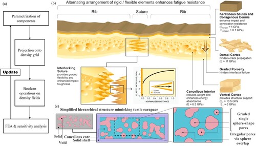
The construction of geometric components is based on the bio-mimicking of the hierarchical structure of the turtle’s carapace rib. As Figure 1(b) shows, the rib of the turtle carapace is composed of the shell region and cancellous core region. The keratinous scutes and collagenous dermis layers are highlighted by the brown and orange shell in the outermost region, which are thin and soft, provide the reinforcement of impact and penetration resistance. The dorsal cortex layer, which is highlighted by the dark yellow shell and adjacent to the collagenous dermis layer, is a stiffer shell that can impede crack propagation. The cancellous core, where the porosity is mainly generated by the nearly spherical pores, can reduce weight and improve energy absorption. The size of pores is geometrically graded, and the shapes of pores can be irregular.

In order to utilise the structural functionalities provided by the turtle’s carapace rib, simplification has been conducted to proceed with the design of bio-mimicking geometric components. Figure 1(c) shows the artificial box structure with several simplifications to facilitate the bio-mimicking. As the left part of Figure 1(c) shows, the simplified structure includes the pores in pink colour and the solid surroundings in grey colour. The keratinous scutes layer, collagenous dermis layer, and dorsal cortex layer are simplified as one single layer of solid. As the middle part of Figure 1(c) shows, the closed-form porosity is guaranteed by the separation of regions, where the outer shell in purple colour is purely solid. The distribution of pores is only allowed inside the inner core region, which is highlighted by the blue region. The cancellous pores are simplified as groups of spheres that can distribute separately or overlap together. The right part of Figure 1(c) shows the partial structure in the core region. The single pores include spheres with different diameters. The irregular pores are generated by the overlap of spheres.

The design of bio-mimicking geometric components is shown in Figure 2. As Figure 2 shows, the set of geometric components includes two types of primitives, which are the solid bar and the hollow sphere. The solid bar is utilised to construct the main structure at the macro level. The spheres are utilised to mimic the cancellous features inside the bar at the micro level. The Figure 2(a) shows the cross-section view of bar and sphere components along the longitudinal direction. Figure 2(b) shows the cross-section view of bar and sphere components in the radial direction. As Figure 2(a) shows, the bar component is composed of a shell region in grey and a core region in pink. Both the shell and core are solid. The shell is generated by the subtraction of the solid core from the enlarged solid bar. The sphere component, which is shown as a green circle in Figure 2(a), is located along the longitudinal direction of the bar component. The core of the bar is classified into three regions, which are the left fillet region, the right fillet region, and the middle polygon region.

Figure 2. Parametrisation of bar-sphere components: (a) Cross-section view of bar and sphere components along longitudinal direction, (b) Cross-section view of the bar-sphere component along the radial direction, (c) Construction of coordinate systems and expression of the bar-sphere component in 3D, (d) Compositions of the bar-sphere component.

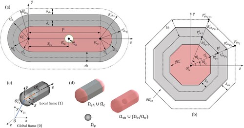
As Figure 2(c) shows, the representation of the bar and sphere are in hierarchical coordinate systems. The bar component is constructed in the global cartesian coordinate system, which is the frame $\left\{0\right\}$ in Figure 2(c). The sphere component is constructed in the local coordinate system, which is the frame $\left\{1\right\}$ in Figure 2(c). Figure 2(d) shows the compositions of components, where the completely pink bio-mimicking component is generated from the boolean operations on the bar component, which is shown in pink and grey, and the sphere component, which is shown in grey colour.

The movement of the bar includes the translation and rotation. As Figure 2(a and c) show, the translational movement of $i^{\mathrm{t}\mathrm{h}}$ bar is controlled by the coordinates of point $O_{c_1}^i$, which can be represented as $\left\{x_{O_{c_1}^i},y_{O_{c_1}^i},z_{O_{c_1}^i}\right\}$or $v_{01}$in the vector form. The rotational movement of $i^{\mathrm{t}\mathrm{h}}$ bar is controlled by the length $l^i$ between point $O_{c_1}^i$ and point $O_{c_2}^i$. As Figure 2(a and c) shows, the length $l^i$ is always along the $\overline{x}$-direction in the local frame $\left\{1\right\}$. In the proposed method, the local frame $\left\{1\right\}$ is constructed by the rotation and translation of the global cartesian frame $\left\{0\right\}$. The rotation of the bar is completely related to the construction of the local frame $\left\{1\right\}$. The construction of the local frame $\left\{1\right\}$ from the global frame $\left\{0\right\}$ is represented in the following equation: (1) $\begin{array}{r}\underset{v^{\left(0\right)}}{\underbrace{\left[\begin{array}{c}x\\ y\\ z\end{array}\right]}}=\underset{R_x}{\underbrace{\left[\begin{array}{c}100\\ 0\cos {\theta }_x\sin {\theta }_x\\ 0-\sin {\theta }_x\cos {\theta }_x\end{array}\right]}}\underset{R_y}{\underbrace{\left[\begin{array}{c}\cos {\theta }_{y}0\sin {\theta }_y\\ 010\\ -\sin {\theta }_{y}0\cos {\theta }_y\end{array}\right]}}\\ \underset{R_z}{\underbrace{\left[\begin{array}{c}\cos {\theta }_z\sin {\theta }_{z}0\\ -\sin {\theta }_z\cos {\theta }_{z}0\\ 001\end{array}\right]}}\underset{v^{\left(1\right)}}{\underbrace{\left[\begin{array}{c}\overline{x}\\ \overline{y}\\ \overline{z}\end{array}\right]}}+\underset{v_{01}}{\underbrace{\left[\begin{array}{c}{x}_{O_{c_1}^i}\\ y_{O_{c_1}^i}\\ z_{O_{c_1}^i}\end{array}\right]}}\end{array}$(1) where the $v^{\left(0\right)}$ is the arbitrary vector in the space in the global frame $\left\{0\right\}$, $R_x$ is the rotation matrix that represents the rotation of the frame along $x$-direction, $R_y$ is the rotation matrix that represents the rotation of frame along $y$-direction, $R_z$ is the rotation matrix that represents the rotation of frame along $z$-direction, $v^{\left(1\right)}$ is the same vector in the local frame $\left\{1\right\}$, and $v_{01}$ is the translation vector that represents the translational movement of the frame.

As Equation (1)(1) $\begin{array}{r}\underset{v^{\left(0\right)}}{\underbrace{\left[\begin{array}{c}x\\ y\\ z\end{array}\right]}}=\underset{R_x}{\underbrace{\left[\begin{array}{c}100\\ 0\cos {\theta }_x\sin {\theta }_x\\ 0-\sin {\theta }_x\cos {\theta }_x\end{array}\right]}}\underset{R_y}{\underbrace{\left[\begin{array}{c}\cos {\theta }_{y}0\sin {\theta }_y\\ 010\\ -\sin {\theta }_{y}0\cos {\theta }_y\end{array}\right]}}\\ \underset{R_z}{\underbrace{\left[\begin{array}{c}\cos {\theta }_z\sin {\theta }_{z}0\\ -\sin {\theta }_z\cos {\theta }_{z}0\\ 001\end{array}\right]}}\underset{v^{\left(1\right)}}{\underbrace{\left[\begin{array}{c}\overline{x}\\ \overline{y}\\ \overline{z}\end{array}\right]}}+\underset{v_{01}}{\underbrace{\left[\begin{array}{c}{x}_{O_{c_1}^i}\\ y_{O_{c_1}^i}\\ z_{O_{c_1}^i}\end{array}\right]}}\end{array}$(1) shows, arbitrary points represented in frame $\left\{1\right\}$ can be expressed in the global frame $\left\{0\right\}$ after rotations along $xyz$-direction and the translation $v_{01}$. When this frame transformation applies to the local length $l^i$, the local length vector $\left(l^i,0,0\right)$ will rotate along $xyz$-direction with respect to the rotation angle $\left\{{\theta }_x,{\theta }_y,{\theta }_z\right\}$, leading to the rotation of the geometric component. The bar is also morphable with the sphere fillet and polygon control.

As Figure 2(b) shows, the shape of $i^{\mathrm{t}\mathrm{h}}$ bar in the left fillet and right fillet region is controlled by the left fillet radius $R_{c_1}^i$and the right fillet radius $R_{c_2}^i$, respectively. The shape middle region of the $i^{\mathrm{t}\mathrm{h}}$ bar is extruded from polygon profile shown in Figure 2(b), where the distance $R_{p_j}^i$ between each polygon vertex $P_j^i$ and the left centre $O_{c_1}^i$ can be manipulated to provide further control of bar shape. The polygon profile can also be utilised to approximate smooth circular profile by decreasing the angular distance, which is expressed as ${\theta }_{p_j}^i=\left(j-1\right)2\pi /n_p$ with total $n_p$ polygon vertices.

As the design variables at the macro level, the set of design variables that control the $i^{\mathrm{t}\mathrm{h}}$ bar component is shown as follows: (2) $x_b^{\left(i\right)}=\left\{x_{O_{c_1}^i},y_{O_{c_1}^i},z_{O_{c_1}^i},{\theta }_x,{\theta }_y,{\theta }_z,l^i,R_{p_1}^i,R_{p_2}^i,\dots ,R_{p_{n_p}}^i,R_{c_1}^i,R_{c_2}^i\right\}$(2) where the $x_b^{\left(i\right)}$ represents the set of bar design variables, the $\left\{x_{O_{c_1}^i},y_{O_{c_1}^i},z_{O_{c_1}^i}\right\}$ represents the position of left centre of bar in the global frame, the $\left\{{\theta }_x,{\theta }_y,{\theta }_z\right\}$ represents the rotation of bar in the global frame, the $l^i$ represents the length of bar in the local frame, the $\left\{R_{p_1}^i,R_{p_2}^i,\dots ,R_{p_{n_p}}^i\right\}$ represents the radii of polygon vertices, the $\left\{R_{c_1}^i,R_{c_2}^i\right\}$ represents the radii of spherical fillet, and the $n_p$ represents the number of polygon vertices of each bar. All design variables for bar components in Equation (2)(2) $x_b^{\left(i\right)}=\left\{x_{O_{c_1}^i},y_{O_{c_1}^i},z_{O_{c_1}^i},{\theta }_x,{\theta }_y,{\theta }_z,l^i,R_{p_1}^i,R_{p_2}^i,\dots ,R_{p_{n_p}}^i,R_{c_1}^i,R_{c_2}^i\right\}$(2) are within the pre-defined range during the optimisation process.

The sphere component inside the solid bar is constructed to facilitate the generation of porous features at the micro level. In order to implement the grading of spherical pores and the pores in irregular shape, the size and position of the sphere is regarded as design variables. The pores are demanded to distribute inside the solid bar. Therefore, the translational movement of pores is constructed completely in the local frame $\left\{1\right\}$, leading to the optimisation at the micro level.

As Figure 2(a and c) shows, the position of the $k^{\mathrm{t}\mathrm{h}}$ sphere inside the $i^{\mathrm{t}\mathrm{h}}$ bar is controlled by the local vector $v_{12}$, which can be fully defined by the position ${\overline{x}}_{s_k}^i$ of sphere centre $O_{s_k}^i$ along the longitudinal direction of bar in the local frame. Although the ${\overline{x}}_{s_k}^i$ can represent the movement of the sphere along the $\overline{x}$-direction in the local frame $\left\{1\right\}$, the range of ${\overline{x}}_{s_k}^i$ is difficult to be fixed during the optimisation due to the varying lengths of bars. To reasonably manipulate the position of spheres with varying lengths of bars, the normalised coordinate ${\overline{\xi }}_{s_k}^i$ has been induced as the design variable. The normalised coordinate ${\overline{\xi }}_{s_k}^i$, which is calculated as ${\overline{\xi }}_{s_k}^i={\overline{x}}_{s_k}^i/l^i$, is between 0 and 1. The utilisation of normalised coordinate ${\overline{\xi }}_{s_k}^i$ can effectively limit the sphere to locate within the bar along the longitudinal direction. When the ${\overline{\xi }}_{s_k}^i$ equal to 1, the sphere locates at the right centre $O_{c_2}^i$ of the bar. When the ${\overline{\xi }}_{s_k}^i$ equal to 0, the sphere locates at the left centre $O_{c_1}^i$ of the bar. The movement of spheres in the $\overline{y}$- and $\overline{z}$-directions are eliminated to simplify the complexity of the topology optimisation problem. The radius of the $k^{\mathrm{t}\mathrm{h}}$ sphere inside the $i^{\mathrm{t}\mathrm{h}}$ bar is represented by$R_{s_k}^i$, which is regarded as another design variable to control the size of pores.

As the design variables at the micro level, the set of design variables that control the $n_s$ sphere components inside the $i^{\mathrm{t}\mathrm{h}}$ bar component is shown as follows: (3) $x_s^{\left(i\right)}=\left\{{\overline{\xi }}_{s_1}^i,{\overline{\xi }}_{s_2}^i,\dots ,{\overline{\xi }}_{s_{n_s}}^i,R_{s_1}^i,R_{s_2}^i,\dots ,R_{s_{n_s}}^i\right\}$(3) where the $x_s^{\left(i\right)}$ represents the set of spheres design variables inside the $i^{\mathrm{t}\mathrm{h}}$ bar, the $\left\{{\overline{\xi }}_{s_1}^i,{\overline{\xi }}_{s_2}^i,\dots ,{\overline{\xi }}_{s_{n_s}}^i\right\}$ represents the normalised positions of spheres along the longitudinal direction in the local frame, the $\left\{R_{s_1}^i,R_{s_2}^i,\dots ,R_{s_{n_s}}^i\right\}$ represents the radii of spheres in the local frame, the $n_s$ represents the number of spheres inside each bar. All the design variables for sphere components in Equation (3)(3) $x_s^{\left(i\right)}=\left\{{\overline{\xi }}_{s_1}^i,{\overline{\xi }}_{s_2}^i,\dots ,{\overline{\xi }}_{s_{n_s}}^i,R_{s_1}^i,R_{s_2}^i,\dots ,R_{s_{n_s}}^i\right\}$(3) are within the pre-defined range during the optimisation process. With comparison to the design variables for bar components in Equation (2)(2) $x_b^{\left(i\right)}=\left\{x_{O_{c_1}^i},y_{O_{c_1}^i},z_{O_{c_1}^i},{\theta }_x,{\theta }_y,{\theta }_z,l^i,R_{p_1}^i,R_{p_2}^i,\dots ,R_{p_{n_p}}^i,R_{c_1}^i,R_{c_2}^i\right\}$(2) , the range of design variables for sphere components has a much smaller scale. Therefore, the bar components and sphere components can be set appropriately to design the structure concurrently at different level. It should be noticed that the radii of sphere components are regarded as design variables. Therefore, the size of pores can be manipulated in the proposed approach.

There are also fixed geometric parameters that have impactions on the geometric components but do not work as design variables. The first type of fixed geometric parameter is thickness $th$. During the optimisation, the overlapping of spheres that belongs to different bars can generate hollow pores that can collapse the closed boundary. Therefore, the shell region of the solid bar, which is shown in grey in Figure 2(a and b), is utilised to limit the sphere to locate inside the bar along the radial direction. In the proposed method, the wall thickness $th$ is set to be fixed during optimisation. The shell region is generated from the subtraction of the inner solid core from the outer solid. The outer solid has the same length as the inner core but the enlarged fillet radii and the enlarged radii for polygon vertices. The relationship between enlarged radii to generate the shell region and the radii in the core region is expressed in the following equations: (4) $\begin{array}{r}{R}_{s{h}_1}^i=R_{c_1}^i+th,\\ R_{s{h}_2}^i=R_{c_2}^i+th,\\ R_{s{h}_{p_j}}^i=R_{p_j}^i+th,j=1,\dots ,n_p\end{array}$(4) where the $R_{s{h}_1}^i$is the left fillet radius of the outer solid, the $R_{s{h}_2}^i$is the right fillet radius of the outer solid, the $R_{s{h}_{p_j}}^i$ is the radii of polygon vertices in the outer solid region, the $R_{c_1}^i$is the left fillet radius in the core region, the $R_{c_2}^i$is the right fillet radius in the core region, the $R_{p_j}^i$ is the radii of polygon vertices in the core region, and the $th$ is the thickness of the shell.

The second type of fixed geometric parameters are the offset distances. As Figure 2(a and b) shows, the offsets ${\delta }_c$ is applied to modify the boundary of core $\mathrm{\partial }{\mathrm{\Omega }}_c^i$. The main functionality of inducing offsets is to soften the sharp boundary, which is important in the density projection process and will be further discussed. The relationship between designed radii and actual radii in the core region is expressed in the following equations: (5) $\begin{array}{r}{R}_{c_1}^i=r_{c_1}^i+{\delta }_c,\\ R_{c_2}^i=r_{c_2}^i+{\delta }_c,\\ R_{p_j}^i=r_{p_j}^i+{\delta }_c,j=1,\dots ,n_p\end{array}$(5) where the $r_{c_1}^i$ is the actual left fillet radius in the core region, the $r_{c_2}^i$ is the actual right fillet radius in the core region, the $r_{p_j}^i$ is the actual radii of polygon vertices in the core region, and $\left\{R_{c_1}^i,R_{c_2}^i,R_{p_1}^i,R_{p_2}^i,\dots ,R_{p_{n_p}}^i\right\}$ are the related designed radii. Similarly, the offset ${\delta }_{sh}$ is applied to modify the boundary of the shell $\mathrm{\partial }{\mathrm{\Omega }}_{sh}^i$. The relationship between designed radii and actual radii in the shell region is expressed in the following equations: (6) $\begin{array}{r}{R}_{s{h}_1}^i=r_{s{h}_1}^i+{\delta }_{sh},\\ R_{s{h}_2}^i=r_{c_2}^i+{\delta }_{sh},\\ R_{s{h}_{p}j}^i=r_{s{h}_{p}j}^i+{\delta }_{sh},j=1,\dots ,n_p\end{array}$(6) where the $r_{s{h}_1}^i$ is the actual left fillet radius in the shell region, the $r_{s{h}_2}^i$ is the actual right fillet radius in the shell region, the $r_{s{h}_{p}j}^i$ is the actual radii of polygon vertices in the shell region, and $\left\{R_{s{h}_1}^i,R_{s{h}_2}^i,R_{s{h}_{p}1}^i,R_{s{h}_{p}2}^i,\dots ,R_{s{h}_p{n}_p}^i\right\}$ are the related designed radii in the shell region. The offset ${\delta }_s$ is applied to the sphere components. The relationship between designed radii and actual radii for spheres is calculated as follows: (7) $R_{s_k}^i=r_{s_k}^i+{\delta }_s,k=1,\dots ,n_s$(7) where the $r_{s_k}^i$ is the actual radius of the sphere, and the $R_{s_k}^i$is the related designed sphere radius.

In conclusion, the thickness and offset distances are fixed parameters that are pre-determined before optimisation. The design variables that are updated according to the sensitivity analysis during optimisation are expressed as follows: (8) $x_{\mathrm{m}\mathrm{u}\mathrm{l}\mathrm{t}\mathrm{i}\mathrm{s}\mathrm{c}\mathrm{a}\mathrm{l}\mathrm{e}}^{\left(i\right)}=\left\{x_b^{\left(i\right)},x_s^{\left(i\right)}\right\},i=1,\dots ,n_b$(8) where the $x_{\mathrm{m}\mathrm{u}\mathrm{l}\mathrm{t}\mathrm{i}\mathrm{s}\mathrm{c}\mathrm{a}\mathrm{l}\mathrm{e}}^{\left(i\right)}$ is the complete set of design variables to design bio-mimicking hierarchical structures, the $x_b^{\left(i\right)}$ is the design variables at the macro level to manipulate the $i^{\mathrm{t}\mathrm{h}}$ bar, the $x_s^{\left(i\right)}$ is the design variables at the micro level to manipulate the $n_s$ spheres, and the $n_b$ is the number of bars. The design variables at both the macro level and the micro level can be adjusted by eliminating or adding specific item. With the reasonable scale separation by setting an appropriate range of design variables. The concurrent multiscale optimisation can be flexibly manipulated.

The density field is essential in the numerical-based evaluation of the design. For the geometric component-based approach, the focus is on the bridge between the geometric design variables and the density of each element in the discretised design space. Figure 3 shows the projection mechanism to generate the density field. The projection is applied to each component before further process. As Figure 3(a) shows, the design space has been discretised into fixed eight-node cubic elements. The minimum distances between the boundary of geometric components and each element are utilised as inputs to further generate the density field via the projection function shown in Figure 3(d). In the proposed method, the inverse density fields of the core region of the bar, the shell region of the bar, and the sphere components are obtained separately at first. As Figure 3(e) shows, the inverse density fields that belong to different regions are then processed to obtain the complete field of the component. The inverse density fields for each component are assembled with further Boolean operations to obtain the inverse density field of the designed structure.

Figure 3. Generation of density field: (a) Illustrations of density elements and bar-sphere components in 3D space, (b) Evaluation of the distance between the element and geometric boundary at the spherical end of the bar, (c) Evaluation of the distance between element and geometric boundary at the middle polygon region of the bar, (d) The projection function to generate density field, (e) Illustration of the inverse density field after projection.

The minimum distances between boundary and elements are calculated in different ways for the bar components. As Figure 3(b) shows, the minimum distance at the spherical fillet region depends on the radius of the fillet. The minimum distance between elements and boundary of bar components in the fillet region can be expressed as follows: (9) $d_k=\Vert v_e\Vert -r_k$(9) where the $d_k$ is the minimum distance in the fillet region, $\Vert v_e\Vert$ is the distance between elements and the fillet centre of the bar, and the $r_k$ is the radius of the fillet. The fillet centre is the point $O_{c_1}^i$ when calculating in the left fillet and the point $O_{c_2}^i$ when calculating the right fillet. In the middle polygon extrusion region of the bar component, the minimum distances occur inside the profile plane, which is the $\overline{y}\overline{z}$-plane shown in Figure 3(a). Figure 3(c) shows the calculation of minimum distance in the polygon extrusion region, where the distance mainly depends on the positions of polygon vertices. The minimum distance between elements and boundary for $j^{\mathrm{t}\mathrm{h}}$ polygon edgy $P_j{P}_{j+1}$ can be expressed as follows: (10) $d_k=\{\begin{array}{c}\begin{array}{c}\Vert v_1\Vert ,v_1\cdot v_3<0\end{array}\\ \begin{array}{c}\Vert v_2\Vert ,0\le v_1\cdot v_3<\Vert P_j{P}_{j+1}\Vert \end{array}\end{array}$(10) where the $d_k$ is the minimum distance in the polygon profile extrusion region, the $\Vert v_1\Vert$ is the distance between elements and the $j^{\mathrm{t}\mathrm{h}}$ polygon vertex $P_j$, the $\Vert v_2\Vert$ is the normal distance between elements and the $j^{\mathrm{t}\mathrm{h}}$ polygon edge $P_j{P}_{j+1}$, the $v_3$ is the unit vector along the $P_j{P}_{j+1}$ direction.

The minimum distance for sphere components can be calculated similarly to the calculation in the fillet region. The minimum distance for sphere components is expressed in the following: (11) $d_k=\Vert v_s\Vert -r_{s_k}^i$(11) where the $d_k$ is the minimum distance field for the sphere components, the $\Vert v_s\Vert$ is the distance between elements and the centre of spheres $O_{s_k}^i$, and the $r_{s_k}^i$ is the actual radius of spheres.

The projection function shown in Figure 3(d) can transform the minimum distance field $d_k$ into an inverse density field ${\phi }_k$ that ranges from 0 to 1, where 0 represents solid and 1 represents void. The utilisation of inverse density ${\phi }_k$ is to support the assembly of all components after projection. The actual density field can be calculated as ${\rho }_k=1-{\phi }_k$ for further finite element analysis, where 0 represents void and 1 represents solid material. The projection function is based on the modification of the sigmoid function and can be expressed as follows: (12) ${\phi }_k={\displaystyle \frac{1}{1+\exp \left[-\alpha \left(-d_k+\delta \right)\right]}}$(12) where the ${\phi }_k$ represents the inverse density for $k^{\mathrm{t}\mathrm{h}}$ component, the $d_k$ represents the minimum distance for $k^{\mathrm{t}\mathrm{h}}$ component, the $\alpha$ is the tuning parameter to sheer the grading rate of the projection function, and the $\delta$ represents the distance offset to soften the density field. The $\delta$ is equal to ${\delta }_c$, ${\delta }_{sh}$, and ${\delta }_s$ when applied to core, shell, and sphere regions, respectively. The projection function illustrated in Equation (12)(12) ${\phi }_k={\displaystyle \frac{1}{1+\exp \left[-\alpha \left(-d_k+\delta \right)\right]}}$(12) constructs the bridge between geometric components and the density grids. The deterministic characteristic features of the projection function also provide effective support for the sensitivity analysis for the proposed method. The projected inverse density field of the single bar with one sphere is illustrated in Figure 3(e). As the colour bar shown in Figure 3(e), the solid elements are in dark blue colour whereas the void elements are in yellow colour. As the grading colour shows, the densities gradually change between void and solid in the region adjacent to the boundaries due to the existence of offset.

The mechanism for the assembly of density fields for each component is illustrated in Figure 4. From left to right, the assembly procedures include the generation of the shell, the generation of the porous core, and the generation of the complete structure. The illustration is based on the assembly of two parametrised bar-sphere components that forms an X-shaped cross. The X-shaped cross is obtained by assigning a fixed angular distance between two bar-sphere components that locate at the same point on the specific plane. Before the implementation of operations shown in Figure 4, two steps of preparation need to be facilitated in advance. Firstly, the inverse density fields ${\phi }_k$ of each component can be generated from Equation (12)(12) ${\phi }_k={\displaystyle \frac{1}{1+\exp \left[-\alpha \left(-d_k+\delta \right)\right]}}$(12) separately. Secondly, the density fields of the shell, core, and pores in the overall structure should be obtained separately from the productions of inverse density fields for all components. Although the shell is generated from the subtraction of the inner part from the outer solid, all the fields of the shell below are regarded as the density of purely outer solid that has been enlarged from the inner solid as explained in Equation (4)(4) $\begin{array}{r}{R}_{s{h}_1}^i=R_{c_1}^i+th,\\ R_{s{h}_2}^i=R_{c_2}^i+th,\\ R_{s{h}_{p_j}}^i=R_{p_j}^i+th,j=1,\dots ,n_p\end{array}$(4) . Another clarification is that all the fields of the core are regarded as the density of purely inner solid that has been explained in Equation (4)(4) $\begin{array}{r}{R}_{s{h}_1}^i=R_{c_1}^i+th,\\ R_{s{h}_2}^i=R_{c_2}^i+th,\\ R_{s{h}_{p_j}}^i=R_{p_j}^i+th,j=1,\dots ,n_p\end{array}$(4) .

Figure 4. Boolean operations on bar-sphere components to generate bio-mimicking closed-form porous structures.

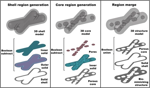
With the density fields of the shell, core, and pores for the overall structure, the assembly of density fields can be completed. As the left part of Figure 4 shows, the generation of the solid shell in grey is from the Boolean subtraction of the blue inner solid, which represents the density of the core, from the purple outer solid, which represents the density of the shell. The 3D shell model shows the result of this step, where the inner solid part has been completely eliminated and is now hollow. As the middle part of Figure 4 shows, the generation of porous core in grey is from the Boolean subtraction of the pink pores, which represents the density of pore, from the blue inner solid, which represents the density of the core. The 3D core model shows the result of this step, where the pores have been eliminated to facilitate the porous features in the core region. As the right part of Figure 4 shows, the generation of complete structure is from the Boolean union of the porous core and solid shell. The 3D structure model shows the result of this step, where the porous core perfectly fills the hollow space of the solid shell. The size and shape of porous region are impacted by the number of spheres inside each bar as well. The smaller number of spheres, e.g. one sphere inside each bar can passively increase the distance between spheres during the optimisation.

The preparation of density fields in the overall structure and the Boolean operations to assembly of the density fields can be expressed as follows: (13) $\begin{array}{r}{\rho }_{sh}=1-\prod _{k=1}^{n_b}{\phi }_{s{h}_k},\\ {\phi }_{s{h}_k}={\displaystyle \frac{1}{1+\exp \left[-\alpha \left(-d_{s{h}_k}+{\delta }_{sh}\right)\right]},}\\ {\rho }_c=1-\prod _{k=1}^{n_b}{\phi }_{c_k},\\ {\phi }_{c_k}={\displaystyle \frac{1}{1+\exp \left[-\alpha \left(-d_{c_k}+{\delta }_c\right)\right]},}\\ {\rho }_s=\prod _{k=1}^{n_b}{\phi }_{s_k},\\ {\phi }_{s_k}={\displaystyle \frac{1}{1+\exp \left[-\alpha \left(-d_{s_k}+{\delta }_s\right)\right]},}\\ {\rho }_{\mathrm{b}\mathrm{i}\mathrm{o}}={\rho }_c\cdot {\rho }_s+{\rho }_{sh}-{\rho }_c\end{array}$(13) where the ${\rho }_{sh}$ is the density field of shell, the ${\rho }_c$ is the density field of core, the ${\rho }_s$ is the density of spheres, the ${\rho }_{\mathrm{b}\mathrm{i}\mathrm{o}}$ is the density of bio-mimicking structure, the ${\phi }_{s{h}_k}$ is the inverse density field of the shell for $k^{\mathrm{t}\mathrm{h}}$ bar, the ${\phi }_{c_k}$is the inverse density field of core for $k^{\mathrm{t}\mathrm{h}}$ bar, the ${\phi }_{s_k}$ is the inverse density field of the hollow pores for spheres inside the $k^{\mathrm{t}\mathrm{h}}$ bar, the $d_{s{h}_k}$ is the minimum distance field of shell for $k^{\mathrm{t}\mathrm{h}}$ bar, the $d_{c_k}$ is the minimum distance field of core for $k^{\mathrm{t}\mathrm{h}}$ bar, the $d_{s_k}$ is the minimum distance field of $k^{\mathrm{t}\mathrm{h}}$ spheres, the $\alpha$ is the tuning parameter, the ${\delta }_{sh}$ is the offset for shell, ${\delta }_c$ is the offset for the core, and the ${\delta }_s$ is the offset for the sphere.

The productions of inverse density fields are vital for the expression of the overall structure. Due to the value of solid elements in inverse density fields being set to 0, the productions of inverse density fields that belong to different components can lead to the union of all solid elements in the design space. It should be noticed that the density field of pores is directly from the productions of inverse density fields without extra operations. That is because the spheres are voids so that the density of pore can be directly expressed by the inverse density fields. After the generation of actual shell density fields, core density fields, and the pores density fields, the density fields for the overall structure can be obtained from boolean operations. The generation of the shell is implemented by the ${\rho }_{sh}-{\rho }_c$ part in the last row of Equation (13)(13) $\begin{array}{r}{\rho }_{sh}=1-\prod _{k=1}^{n_b}{\phi }_{s{h}_k},\\ {\phi }_{s{h}_k}={\displaystyle \frac{1}{1+\exp \left[-\alpha \left(-d_{s{h}_k}+{\delta }_{sh}\right)\right]},}\\ {\rho }_c=1-\prod _{k=1}^{n_b}{\phi }_{c_k},\\ {\phi }_{c_k}={\displaystyle \frac{1}{1+\exp \left[-\alpha \left(-d_{c_k}+{\delta }_c\right)\right]},}\\ {\rho }_s=\prod _{k=1}^{n_b}{\phi }_{s_k},\\ {\phi }_{s_k}={\displaystyle \frac{1}{1+\exp \left[-\alpha \left(-d_{s_k}+{\delta }_s\right)\right]},}\\ {\rho }_{\mathrm{b}\mathrm{i}\mathrm{o}}={\rho }_c\cdot {\rho }_s+{\rho }_{sh}-{\rho }_c\end{array}$(13) . The generation of porous core is implemented by the ${\rho }_c\cdot {\rho }_s$ part in Equation (13)(13) $\begin{array}{r}{\rho }_{sh}=1-\prod _{k=1}^{n_b}{\phi }_{s{h}_k},\\ {\phi }_{s{h}_k}={\displaystyle \frac{1}{1+\exp \left[-\alpha \left(-d_{s{h}_k}+{\delta }_{sh}\right)\right]},}\\ {\rho }_c=1-\prod _{k=1}^{n_b}{\phi }_{c_k},\\ {\phi }_{c_k}={\displaystyle \frac{1}{1+\exp \left[-\alpha \left(-d_{c_k}+{\delta }_c\right)\right]},}\\ {\rho }_s=\prod _{k=1}^{n_b}{\phi }_{s_k},\\ {\phi }_{s_k}={\displaystyle \frac{1}{1+\exp \left[-\alpha \left(-d_{s_k}+{\delta }_s\right)\right]},}\\ {\rho }_{\mathrm{b}\mathrm{i}\mathrm{o}}={\rho }_c\cdot {\rho }_s+{\rho }_{sh}-{\rho }_c\end{array}$(13) . The merge of shell and porous core is implemented by the addition of ${\rho }_{sh}-{\rho }_c$ and ${\rho }_c\cdot {\rho }_s$ in Equation (13)(13) $\begin{array}{r}{\rho }_{sh}=1-\prod _{k=1}^{n_b}{\phi }_{s{h}_k},\\ {\phi }_{s{h}_k}={\displaystyle \frac{1}{1+\exp \left[-\alpha \left(-d_{s{h}_k}+{\delta }_{sh}\right)\right]},}\\ {\rho }_c=1-\prod _{k=1}^{n_b}{\phi }_{c_k},\\ {\phi }_{c_k}={\displaystyle \frac{1}{1+\exp \left[-\alpha \left(-d_{c_k}+{\delta }_c\right)\right]},}\\ {\rho }_s=\prod _{k=1}^{n_b}{\phi }_{s_k},\\ {\phi }_{s_k}={\displaystyle \frac{1}{1+\exp \left[-\alpha \left(-d_{s_k}+{\delta }_s\right)\right]},}\\ {\rho }_{\mathrm{b}\mathrm{i}\mathrm{o}}={\rho }_c\cdot {\rho }_s+{\rho }_{sh}-{\rho }_c\end{array}$(13) .

3. Topology optimisation problem settings

The optimisation problem setting of the proposed method is constructed based on the SIMP method. The main modification is on the embedding of design variables. The geometric parameters are regarded as design variables instead of densities at elements. Another modification is the adjustment of the sensitivity analysis with the minimum distance $d_k$. In order to utilise the versatility of the proposed method, the concurrent multiscale topology optimisation with the manipulation of bar and spheres are applied to resolve the Messershmitt-Bolkow-Blohm (MBB) and L-beam problem. In addition, the topology optimisation of structures at the micro level with the manipulation of spheres is applied to resolve the lattice structure design, where the frames of lattice at the macro level are pre-defined and fixed during optimisation. The lattice structure design includes the simply cubic (SC) lattice design and the octet-truss (OT) unit cell design. In this section, the optimisation problem settings and sensitivity analysis are given for both the multiscale beam design problems and the lattice structure design problems.

3.1. Topology optimisation problem settings for multiscale beam designs

The optimisation problem settings for the classical MBB beam design and L-beam design are based on the SIMP method. For the MBB and L-beam problem, the structure is concurrently optimised with bars at macro level and spheres at the micro level. The minimum structural compliance $c$ is set to be the objective and is given as follows: (14) $c=\sum _{e=1}^{n_e}\left[{\rho }_{min}+{\left({\rho }_{\mathrm{b}\mathrm{i}\mathrm{o}}^{\left(e\right)}\right)}^{\eta }\left(1-{\rho }_{min}\right)\right]u_e^T{k}_0{u}_e$(14) where the ${\rho }_{\mathrm{b}\mathrm{i}\mathrm{o}}^{\left(e\right)}$ is the density of bio-mimicking structure at element $e$ that can be obtained from Equation (13)(13) $\begin{array}{r}{\rho }_{sh}=1-\prod _{k=1}^{n_b}{\phi }_{s{h}_k},\\ {\phi }_{s{h}_k}={\displaystyle \frac{1}{1+\exp \left[-\alpha \left(-d_{s{h}_k}+{\delta }_{sh}\right)\right]},}\\ {\rho }_c=1-\prod _{k=1}^{n_b}{\phi }_{c_k},\\ {\phi }_{c_k}={\displaystyle \frac{1}{1+\exp \left[-\alpha \left(-d_{c_k}+{\delta }_c\right)\right]},}\\ {\rho }_s=\prod _{k=1}^{n_b}{\phi }_{s_k},\\ {\phi }_{s_k}={\displaystyle \frac{1}{1+\exp \left[-\alpha \left(-d_{s_k}+{\delta }_s\right)\right]},}\\ {\rho }_{\mathrm{b}\mathrm{i}\mathrm{o}}={\rho }_c\cdot {\rho }_s+{\rho }_{sh}-{\rho }_c\end{array}$(13) , the ${\rho }_{min}$ is the density at void elements to avoid singularity during optimisation, the $u_e$ is the displacement vector at element $e$ that can be obtained from the FEA, the $k_0$ is the element stiffness matrix, the $\eta$ is the penalty coefficient, and the $n_e$ is the number of elements in the design space.

The optimisation set-up of the minimum compliance problem for MBB beam design and L-beam design is shown in the following: (15) $\begin{array}{r}\begin{array}{c}\underset{x}{min}c\left(x\right)\end{array}\\ \mathrm{s}\mathrm{u}\mathrm{b}\mathrm{j}\mathrm{e}\mathrm{c}\mathrm{t}\mathrm{t}\mathrm{o}Ku=F\\ {\displaystyle \frac{1}{V}\underset{{\mathrm{\Omega }}_0}{\int }{\rho }_{\mathrm{b}\mathrm{i}\mathrm{o}}^{\left(e\right)}dV-f\le 0}\\ -{\displaystyle \frac{1}{V_f}\underset{{\mathrm{\Omega }}_0}{\int }{\rho }_c^{\left(e\right)}\cdot {\rho }_s^{\left(e\right)}dV+p\le 0}\\ x_{min}\le x\le x_{max}\end{array}$(15) where the $x=\left\{x_{\mathrm{m}\mathrm{u}\mathrm{l}\mathrm{t}\mathrm{i}\mathrm{s}\mathrm{c}\mathrm{a}\mathrm{l}\mathrm{e}}^{\left(i\right)}\right\},i=1,\dots ,n_b$ is the set of design variables to manipulate $n_b$ bars and $n_s\cdot n_b$ spheres that has been described in Equation (8)(8) $x_{\mathrm{m}\mathrm{u}\mathrm{l}\mathrm{t}\mathrm{i}\mathrm{s}\mathrm{c}\mathrm{a}\mathrm{l}\mathrm{e}}^{\left(i\right)}=\left\{x_b^{\left(i\right)},x_s^{\left(i\right)}\right\},i=1,\dots ,n_b$(8) in Section 2, the $K$ is the global stiffness matrix that is from the assembly of all element stiffness matrices, the $u$ is the global displacement vector to represent displacements at all elements, the $F$ is the global force vector to represent the load conditions, the $V$ is the volume of the design space ${\mathrm{\Omega }}_0$, the $f$ is the target volume fraction that the optimised design can reach, the $V_f=V\cdot f$ is the target volume of the optimised design, the $p$ is the target porosity of the optimised design should achieve, the $x_{min}$ and $x_{max}$ are the limits of design variables during optimisation.

As Equation (15)(15) $\begin{array}{r}\begin{array}{c}\underset{x}{min}c\left(x\right)\end{array}\\ \mathrm{s}\mathrm{u}\mathrm{b}\mathrm{j}\mathrm{e}\mathrm{c}\mathrm{t}\mathrm{t}\mathrm{o}Ku=F\\ {\displaystyle \frac{1}{V}\underset{{\mathrm{\Omega }}_0}{\int }{\rho }_{\mathrm{b}\mathrm{i}\mathrm{o}}^{\left(e\right)}dV-f\le 0}\\ -{\displaystyle \frac{1}{V_f}\underset{{\mathrm{\Omega }}_0}{\int }{\rho }_c^{\left(e\right)}\cdot {\rho }_s^{\left(e\right)}dV+p\le 0}\\ x_{min}\le x\le x_{max}\end{array}$(15) shows, the bars at the macro level and the spheres at the micro level are optimised for the MBB and L-beam design. For optimising the classical beam problem, the bar component at the macro level can move, morph, and overlap to generate a flexible topology of the structure. The sphere components at the micro level can move, morph, and overlap to generate cancellous infillings that is similar to the rib of a turtle’s carapace. The volume of porous voids can be effectively expressed by ${\rho }_c^{\left(e\right)}\cdot {\rho }_s^{\left(e\right)}$ without aggregation of constraints. The mechanism is described in Equation (13)(13) $\begin{array}{r}{\rho }_{sh}=1-\prod _{k=1}^{n_b}{\phi }_{s{h}_k},\\ {\phi }_{s{h}_k}={\displaystyle \frac{1}{1+\exp \left[-\alpha \left(-d_{s{h}_k}+{\delta }_{sh}\right)\right]},}\\ {\rho }_c=1-\prod _{k=1}^{n_b}{\phi }_{c_k},\\ {\phi }_{c_k}={\displaystyle \frac{1}{1+\exp \left[-\alpha \left(-d_{c_k}+{\delta }_c\right)\right]},}\\ {\rho }_s=\prod _{k=1}^{n_b}{\phi }_{s_k},\\ {\phi }_{s_k}={\displaystyle \frac{1}{1+\exp \left[-\alpha \left(-d_{s_k}+{\delta }_s\right)\right]},}\\ {\rho }_{\mathrm{b}\mathrm{i}\mathrm{o}}={\rho }_c\cdot {\rho }_s+{\rho }_{sh}-{\rho }_c\end{array}$(13) of Section 2. In addition, the spheres that can control the porosity are optimised within related bar components. This limitation, where the spheres are constrained to locate inside bars, can naturally support the porosity to achieve a relevant uniform distribution.

The sensitivity analysis is calculated based on the chain rule and the expression of the density field for the overall structure as shown in Equation (13)(13) $\begin{array}{r}{\rho }_{sh}=1-\prod _{k=1}^{n_b}{\phi }_{s{h}_k},\\ {\phi }_{s{h}_k}={\displaystyle \frac{1}{1+\exp \left[-\alpha \left(-d_{s{h}_k}+{\delta }_{sh}\right)\right]},}\\ {\rho }_c=1-\prod _{k=1}^{n_b}{\phi }_{c_k},\\ {\phi }_{c_k}={\displaystyle \frac{1}{1+\exp \left[-\alpha \left(-d_{c_k}+{\delta }_c\right)\right]},}\\ {\rho }_s=\prod _{k=1}^{n_b}{\phi }_{s_k},\\ {\phi }_{s_k}={\displaystyle \frac{1}{1+\exp \left[-\alpha \left(-d_{s_k}+{\delta }_s\right)\right]},}\\ {\rho }_{\mathrm{b}\mathrm{i}\mathrm{o}}={\rho }_c\cdot {\rho }_s+{\rho }_{sh}-{\rho }_c\end{array}$(13) . The calculation of sensitivity analysis is shown as follows: (16) $\begin{array}{r}{\displaystyle \frac{\mathrm{\partial }c}{\mathrm{\partial }\tau }=\sum _{e=1}^{n_e}{\displaystyle \frac{\mathrm{\partial }c}{\mathrm{\partial }{\rho }_{\mathrm{b}\mathrm{i}\mathrm{o}}^{\left(e\right)}}}}\\ \left[{\displaystyle \frac{\mathrm{\partial }{\rho }_c^{\left(e\right)}}{\mathrm{\partial }{d}_c^{\left(e\right)}}{\displaystyle \frac{\mathrm{\partial }{d}_c^{\left(e\right)}}{\mathrm{\partial }\tau }\left({\rho }_s^{\left(e\right)}-1\right)+{\rho }_c^{\left(e\right)}{\displaystyle \frac{\mathrm{\partial }{\rho }_s^{\left(e\right)}}{\mathrm{\partial }{d}_s^{\left(e\right)}}{\displaystyle \frac{\mathrm{\partial }{d}_s^{\left(e\right)}}{\mathrm{\partial }\tau }+{\displaystyle \frac{\mathrm{\partial }{\rho }_{sh}^{\left(e\right)}}{\mathrm{\partial }{d}_{sh}^{\left(e\right)}}{\displaystyle \frac{\mathrm{\partial }{d}_{sh}^{\left(e\right)}}{\mathrm{\partial }\tau }}}}}}}\right]\end{array}$(16) where the $\tau$ is each design variable in the set $x$ in Equation (15)(15) $\begin{array}{r}\begin{array}{c}\underset{x}{min}c\left(x\right)\end{array}\\ \mathrm{s}\mathrm{u}\mathrm{b}\mathrm{j}\mathrm{e}\mathrm{c}\mathrm{t}\mathrm{t}\mathrm{o}Ku=F\\ {\displaystyle \frac{1}{V}\underset{{\mathrm{\Omega }}_0}{\int }{\rho }_{\mathrm{b}\mathrm{i}\mathrm{o}}^{\left(e\right)}dV-f\le 0}\\ -{\displaystyle \frac{1}{V_f}\underset{{\mathrm{\Omega }}_0}{\int }{\rho }_c^{\left(e\right)}\cdot {\rho }_s^{\left(e\right)}dV+p\le 0}\\ x_{min}\le x\le x_{max}\end{array}$(15) , the $d_c^{\left(e\right)}$is the minimum distance filed for the core region at element $e$, the $d_{sh}^{\left(e\right)}$ is the minimum distance field for shell, the $d_s^{\left(e\right)}$ is the minimum distance field for the sphere. The $\mathrm{\partial }c/\mathrm{\partial }{\rho }_{\mathrm{b}\mathrm{i}\mathrm{o}}^{\left(e\right)}$ part is derived from the adjoint method: (17) ${\displaystyle \frac{\mathrm{\partial }c}{{\rho }_{\mathrm{b}\mathrm{i}\mathrm{o}}^{\left(e\right)}}=-\eta \left({\rho }_{\mathrm{b}\mathrm{i}\mathrm{o}}^{\left(e\right)}{)}^{\eta -1}\right(1-{\rho }_{min})u_e^T{k}_0{u}_e}$(17) The $\mathrm{\partial }{\rho }_c^{\left(e\right)}/\mathrm{\partial }{d}_c^{\left(e\right)}$, $\mathrm{\partial }{\rho }_{sh}^{\left(e\right)}/\mathrm{\partial }{d}_{sh}^{\left(e\right)}$, and $\mathrm{\partial }{\rho }_s^{\left(e\right)}/\mathrm{\partial }{d}_s^{\left(e\right)}$ terms are related to the projection process. These projection terms can be obtained from Equation (13)(13) $\begin{array}{r}{\rho }_{sh}=1-\prod _{k=1}^{n_b}{\phi }_{s{h}_k},\\ {\phi }_{s{h}_k}={\displaystyle \frac{1}{1+\exp \left[-\alpha \left(-d_{s{h}_k}+{\delta }_{sh}\right)\right]},}\\ {\rho }_c=1-\prod _{k=1}^{n_b}{\phi }_{c_k},\\ {\phi }_{c_k}={\displaystyle \frac{1}{1+\exp \left[-\alpha \left(-d_{c_k}+{\delta }_c\right)\right]},}\\ {\rho }_s=\prod _{k=1}^{n_b}{\phi }_{s_k},\\ {\phi }_{s_k}={\displaystyle \frac{1}{1+\exp \left[-\alpha \left(-d_{s_k}+{\delta }_s\right)\right]},}\\ {\rho }_{\mathrm{b}\mathrm{i}\mathrm{o}}={\rho }_c\cdot {\rho }_s+{\rho }_{sh}-{\rho }_c\end{array}$(13) . The $\mathrm{\partial }{d}_c^{\left(e\right)}/\mathrm{\partial }{\tau }_k$, $\mathrm{\partial }{d}_{sh}^{\left(e\right)}/\mathrm{\partial }{\tau }_k$, and $\mathrm{\partial }{d}_s^{\left(e\right)}/\mathrm{\partial }{\tau }_k$ terms are related to the parametrisation of components. These parametrisation terms can be obtained from Equation (9)(9) $d_k=\Vert v_e\Vert -r_k$(9) and Equation (10)(10) $d_k=\{\begin{array}{c}\begin{array}{c}\Vert v_1\Vert ,v_1\cdot v_3<0\end{array}\\ \begin{array}{c}\Vert v_2\Vert ,0\le v_1\cdot v_3<\Vert P_j{P}_{j+1}\Vert \end{array}\end{array}$(10) .

3.2. Topology optimisation problem settings for lattice structure designs

The optimisation problem settings for the simply cubic (SC) lattice structure design and octet-truss (OT) unit cell design are based on the SIMP method. The minimum structural compliance $c$ is set to be the objective and is completely same as the Equation (14)(14) $c=\sum _{e=1}^{n_e}\left[{\rho }_{min}+{\left({\rho }_{\mathrm{b}\mathrm{i}\mathrm{o}}^{\left(e\right)}\right)}^{\eta }\left(1-{\rho }_{min}\right)\right]u_e^T{k}_0{u}_e$(14) shows.

The optimisation set-up of the minimum compliance problem for simply cubic lattice design and octet truss unit cell design is shown in the following: (18) $\begin{array}{r}\begin{array}{c}\underset{x}{min}c\left(x\right)\end{array}\\ \mathrm{s}\mathrm{u}\mathrm{b}\mathrm{j}\mathrm{e}\mathrm{c}\mathrm{t}\mathrm{t}\mathrm{o}Ku=F\\ -{\displaystyle \frac{1}{V_f}\underset{{\mathrm{\Omega }}_0}{\int }{\rho }_c^{\left(e\right)}\cdot {\rho }_s^{\left(e\right)}dV+p\le 0}\\ x_{min}\le x\le x_{max}\end{array}$(18) where the $x=\left\{x_s^{\left(i\right)}\right\},i=1,\dots ,n_b$ is the set of design variables to only manipulate $n_s\cdot n_b$ spheres that have been described in Equation (8)(8) $x_{\mathrm{m}\mathrm{u}\mathrm{l}\mathrm{t}\mathrm{i}\mathrm{s}\mathrm{c}\mathrm{a}\mathrm{l}\mathrm{e}}^{\left(i\right)}=\left\{x_b^{\left(i\right)},x_s^{\left(i\right)}\right\},i=1,\dots ,n_b$(8) of Section 2. The remaining parameters in Equation (16)(16) $\begin{array}{r}{\displaystyle \frac{\mathrm{\partial }c}{\mathrm{\partial }\tau }=\sum _{e=1}^{n_e}{\displaystyle \frac{\mathrm{\partial }c}{\mathrm{\partial }{\rho }_{\mathrm{b}\mathrm{i}\mathrm{o}}^{\left(e\right)}}}}\\ \left[{\displaystyle \frac{\mathrm{\partial }{\rho }_c^{\left(e\right)}}{\mathrm{\partial }{d}_c^{\left(e\right)}}{\displaystyle \frac{\mathrm{\partial }{d}_c^{\left(e\right)}}{\mathrm{\partial }\tau }\left({\rho }_s^{\left(e\right)}-1\right)+{\rho }_c^{\left(e\right)}{\displaystyle \frac{\mathrm{\partial }{\rho }_s^{\left(e\right)}}{\mathrm{\partial }{d}_s^{\left(e\right)}}{\displaystyle \frac{\mathrm{\partial }{d}_s^{\left(e\right)}}{\mathrm{\partial }\tau }+{\displaystyle \frac{\mathrm{\partial }{\rho }_{sh}^{\left(e\right)}}{\mathrm{\partial }{d}_{sh}^{\left(e\right)}}{\displaystyle \frac{\mathrm{\partial }{d}_{sh}^{\left(e\right)}}{\mathrm{\partial }\tau }}}}}}}\right]\end{array}$(16) are completely the same as the definitions in Equation (15)(15) $\begin{array}{r}\begin{array}{c}\underset{x}{min}c\left(x\right)\end{array}\\ \mathrm{s}\mathrm{u}\mathrm{b}\mathrm{j}\mathrm{e}\mathrm{c}\mathrm{t}\mathrm{t}\mathrm{o}Ku=F\\ {\displaystyle \frac{1}{V}\underset{{\mathrm{\Omega }}_0}{\int }{\rho }_{\mathrm{b}\mathrm{i}\mathrm{o}}^{\left(e\right)}dV-f\le 0}\\ -{\displaystyle \frac{1}{V_f}\underset{{\mathrm{\Omega }}_0}{\int }{\rho }_c^{\left(e\right)}\cdot {\rho }_s^{\left(e\right)}dV+p\le 0}\\ x_{min}\le x\le x_{max}\end{array}$(15) . The bar components that construct the lattice frame are fixed during optimisation.

As Equation (16)(16) $\begin{array}{r}{\displaystyle \frac{\mathrm{\partial }c}{\mathrm{\partial }\tau }=\sum _{e=1}^{n_e}{\displaystyle \frac{\mathrm{\partial }c}{\mathrm{\partial }{\rho }_{\mathrm{b}\mathrm{i}\mathrm{o}}^{\left(e\right)}}}}\\ \left[{\displaystyle \frac{\mathrm{\partial }{\rho }_c^{\left(e\right)}}{\mathrm{\partial }{d}_c^{\left(e\right)}}{\displaystyle \frac{\mathrm{\partial }{d}_c^{\left(e\right)}}{\mathrm{\partial }\tau }\left({\rho }_s^{\left(e\right)}-1\right)+{\rho }_c^{\left(e\right)}{\displaystyle \frac{\mathrm{\partial }{\rho }_s^{\left(e\right)}}{\mathrm{\partial }{d}_s^{\left(e\right)}}{\displaystyle \frac{\mathrm{\partial }{d}_s^{\left(e\right)}}{\mathrm{\partial }\tau }+{\displaystyle \frac{\mathrm{\partial }{\rho }_{sh}^{\left(e\right)}}{\mathrm{\partial }{d}_{sh}^{\left(e\right)}}{\displaystyle \frac{\mathrm{\partial }{d}_{sh}^{\left(e\right)}}{\mathrm{\partial }\tau }}}}}}}\right]\end{array}$(16) shows, the structure at the macro level for the SC lattice and OT unit cell are pre-determined before optimisation. The structure at macro level, which are the position and diameters of the truss, does not change during the optimisation. As a result, only the spheres at the micro level are manipulated to achieve the optimised distribution of pores inside the truss-based lattice structure. There are no volume fraction constraints that is existing in the classical beam optimisation problem.

The sensitivity analysis is only related to the control of spheres, where the bar components do not contribute to the sensitivity analysis. The sensitivity analysis can be calculated as: (19) ${\displaystyle \frac{\mathrm{\partial }c}{\mathrm{\partial }\tau }=\sum _{e=1}^{n_e}{\displaystyle \frac{\mathrm{\partial }c}{\mathrm{\partial }{\rho }_{\mathrm{b}\mathrm{i}\mathrm{o}}^{\left(e\right)}}{\displaystyle \frac{\mathrm{\partial }{\rho }_s^{\left(e\right)}}{\mathrm{\partial }{d}_s^{\left(e\right)}}{\displaystyle \frac{\mathrm{\partial }{d}_s^{\left(e\right)}}{\mathrm{\partial }\tau }}}}{\rho }_c^{\left(e\right)}}$(19) where the $\tau$ is each design variable in the set $x$ in Equation (18)(18) $\begin{array}{r}\begin{array}{c}\underset{x}{min}c\left(x\right)\end{array}\\ \mathrm{s}\mathrm{u}\mathrm{b}\mathrm{j}\mathrm{e}\mathrm{c}\mathrm{t}\mathrm{t}\mathrm{o}Ku=F\\ -{\displaystyle \frac{1}{V_f}\underset{{\mathrm{\Omega }}_0}{\int }{\rho }_c^{\left(e\right)}\cdot {\rho }_s^{\left(e\right)}dV+p\le 0}\\ x_{min}\le x\le x_{max}\end{array}$(18) , the $d_s^{\left(e\right)}$ is the minimum distance field for sphere. The $\mathrm{\partial }c/\mathrm{\partial }{\rho }_{\mathrm{b}\mathrm{i}\mathrm{o}}^{\left(e\right)}$ part is derived from the adjoint method in Equation (17)(17) ${\displaystyle \frac{\mathrm{\partial }c}{{\rho }_{\mathrm{b}\mathrm{i}\mathrm{o}}^{\left(e\right)}}=-\eta \left({\rho }_{\mathrm{b}\mathrm{i}\mathrm{o}}^{\left(e\right)}{)}^{\eta -1}\right(1-{\rho }_{min})u_e^T{k}_0{u}_e}$(17) .

The $\mathrm{\partial }{\rho }_s^{\left(e\right)}/\mathrm{\partial }{d}_s^{\left(e\right)}$ term is related to the projection process and can be obtained from Equation (13)(13) $\begin{array}{r}{\rho }_{sh}=1-\prod _{k=1}^{n_b}{\phi }_{s{h}_k},\\ {\phi }_{s{h}_k}={\displaystyle \frac{1}{1+\exp \left[-\alpha \left(-d_{s{h}_k}+{\delta }_{sh}\right)\right]},}\\ {\rho }_c=1-\prod _{k=1}^{n_b}{\phi }_{c_k},\\ {\phi }_{c_k}={\displaystyle \frac{1}{1+\exp \left[-\alpha \left(-d_{c_k}+{\delta }_c\right)\right]},}\\ {\rho }_s=\prod _{k=1}^{n_b}{\phi }_{s_k},\\ {\phi }_{s_k}={\displaystyle \frac{1}{1+\exp \left[-\alpha \left(-d_{s_k}+{\delta }_s\right)\right]},}\\ {\rho }_{\mathrm{b}\mathrm{i}\mathrm{o}}={\rho }_c\cdot {\rho }_s+{\rho }_{sh}-{\rho }_c\end{array}$(13) . The $\mathrm{\partial }{d}_s^{\left(e\right)}/\mathrm{\partial }{\tau }_k$ term is related to the parametrisation of components and can be obtained from Equation (9)(9) $d_k=\Vert v_e\Vert -r_k$(9) and Equation (10)(10) $d_k=\{\begin{array}{c}\begin{array}{c}\Vert v_1\Vert ,v_1\cdot v_3<0\end{array}\\ \begin{array}{c}\Vert v_2\Vert ,0\le v_1\cdot v_3<\Vert P_j{P}_{j+1}\Vert \end{array}\end{array}$(10) .

4. Numerical examples

In this section, concurrent multiscale structural optimisation and lattice structure optimisation examples are illustrated to validate the proposed method. The objective is to find the minimum of compliance as shown in Equation (15)(15) $\begin{array}{r}\begin{array}{c}\underset{x}{min}c\left(x\right)\end{array}\\ \mathrm{s}\mathrm{u}\mathrm{b}\mathrm{j}\mathrm{e}\mathrm{c}\mathrm{t}\mathrm{t}\mathrm{o}Ku=F\\ {\displaystyle \frac{1}{V}\underset{{\mathrm{\Omega }}_0}{\int }{\rho }_{\mathrm{b}\mathrm{i}\mathrm{o}}^{\left(e\right)}dV-f\le 0}\\ -{\displaystyle \frac{1}{V_f}\underset{{\mathrm{\Omega }}_0}{\int }{\rho }_c^{\left(e\right)}\cdot {\rho }_s^{\left(e\right)}dV+p\le 0}\\ x_{min}\le x\le x_{max}\end{array}$(15) and Equation (18)(18) $\begin{array}{r}\begin{array}{c}\underset{x}{min}c\left(x\right)\end{array}\\ \mathrm{s}\mathrm{u}\mathrm{b}\mathrm{j}\mathrm{e}\mathrm{c}\mathrm{t}\mathrm{t}\mathrm{o}Ku=F\\ -{\displaystyle \frac{1}{V_f}\underset{{\mathrm{\Omega }}_0}{\int }{\rho }_c^{\left(e\right)}\cdot {\rho }_s^{\left(e\right)}dV+p\le 0}\\ x_{min}\le x\le x_{max}\end{array}$(18) . The solid material is assumed to be isotropic. The optimisation is within the elastic region and Young’s modulus is set to be $E_0=1$. The Poisson’s ratio is set to be ${\nu }_0=0.3$. The element stiffness matrix $k_0$ is constructed based on the $E_0$ and the ${\nu }_0$. In the proposed method, the density at void elements ${\rho }_{min}$ is set to be $1e-4$ to avoid singularities. The penalty coefficient $\eta$ is set to be 3. The projection tuning parameter $\alpha$ in Equation (13)(13) $\begin{array}{r}{\rho }_{sh}=1-\prod _{k=1}^{n_b}{\phi }_{s{h}_k},\\ {\phi }_{s{h}_k}={\displaystyle \frac{1}{1+\exp \left[-\alpha \left(-d_{s{h}_k}+{\delta }_{sh}\right)\right]},}\\ {\rho }_c=1-\prod _{k=1}^{n_b}{\phi }_{c_k},\\ {\phi }_{c_k}={\displaystyle \frac{1}{1+\exp \left[-\alpha \left(-d_{c_k}+{\delta }_c\right)\right]},}\\ {\rho }_s=\prod _{k=1}^{n_b}{\phi }_{s_k},\\ {\phi }_{s_k}={\displaystyle \frac{1}{1+\exp \left[-\alpha \left(-d_{s_k}+{\delta }_s\right)\right]},}\\ {\rho }_{\mathrm{b}\mathrm{i}\mathrm{o}}={\rho }_c\cdot {\rho }_s+{\rho }_{sh}-{\rho }_c\end{array}$(13) is set to 6.

4.1. Multiscale bio-mimicking Messershmitt-Bolkow-Blohm (MBB)

For the validation of the proposed multiscale bio-mimicking structural optimisation method, the MBB beams with minimal compliance are designed. As Figure 5(a) shows, the size of the design space is $300\times 100\times 20$. The half of the beam along the $x$-direction is constructed with the symmetric boundary condition to simplify the problem. The point load in the negative $y$-direction is applied to the middle of the top left edge. The degree of freedoms in the $x$-direction are fixed for the nodes on the left surface to facilitate symmetric boundary condition. The degree of freedoms in the $y$-direction is fixed for the nodes on the bottom right edge as support.

Figure 5. Multiscale Messershmitt-Bolkow-Blohm (MBB) problem: (a) The definition of MBB problem, (b) Initial design of MBB in isometric transparent view, (c) The optimised design of MBB with 0.06 porosity.

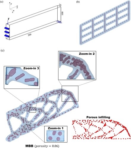
For the multiscale MBB problem, 171 bar components and 342 sphere components are manipulated to optimise the bio-mimicking porous structure. As Figure 5(b) shows, the initial design consists of 171 bars located in the horizontal and vertical directions at the macro level. In the horizontal direction, there are total 4 rows of truss, where each row is composed of 24 horizontal bars. In the vertical direction, there total 5 columns of truss, where each column is composed of 15 vertical bars. The cross-section profile of each bar is controlled by 24 polygon vertices. There are two spheres inside each bar at the micro level for the generation of voids. The two spheres are located at two endpoints of bar components. Therefore, the spheres shown in Figure 5(b) overlapped at some locations.

The volume of the structure is constrained by setting the target volume fraction $f$ equal to 0.3. The target porosity $p$, which is the volume ratio of porous infillings to the solid truss-based structure, is set to 0.06, 0.08, and 0.10, respectively. The two constraints need to reach the target after the optimisation.

Figure 5(c) shows the optimised MBB beam under the 0.06 porosity constraints, where the voids take 6% volume inside the beam. From the observation of the red-highlighted porous infilling shown in Figure 5(c), a certain degree of uniform distribution of voids has been achieved. Another observation is that the voids are not strictly regularly arranged, leading to the achievement of stochastic porous infillings design. The morphology of voids is illustrated in the zoom-in parts of Figure 5(c). The three zoom-in parts show the typical types of morphologies, where zoom-in 1 illustrates the spherical voids that are distributed separately, zoom-in 2 illustrates the void cluster that is generated from the overlap of large quantities of spheres, and zoom-in 3 illustrates the stripe void that is generated form the overlap of several spheres. Both separate regular voids and irregular voids can be obtained by the proposed method.

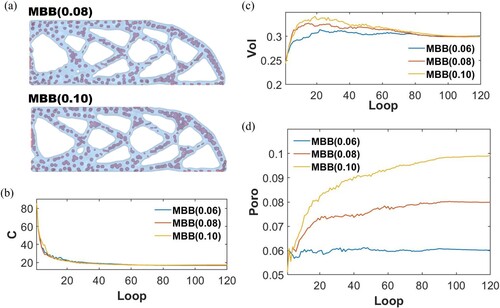
Figure 6(a) shows the optimised MBB with 0.08 and 0.10 porosity constraints. Both optimised designs can achieve the expected pores distribution and the void morphology as the 0.06 porosity design. From the observations of pores distribution, the low porosity target design owns smaller size of pores. The porosity control is embedded in the global constraint, which is shown in Equation (15)(15) $\begin{array}{r}\begin{array}{c}\underset{x}{min}c\left(x\right)\end{array}\\ \mathrm{s}\mathrm{u}\mathrm{b}\mathrm{j}\mathrm{e}\mathrm{c}\mathrm{t}\mathrm{t}\mathrm{o}Ku=F\\ {\displaystyle \frac{1}{V}\underset{{\mathrm{\Omega }}_0}{\int }{\rho }_{\mathrm{b}\mathrm{i}\mathrm{o}}^{\left(e\right)}dV-f\le 0}\\ -{\displaystyle \frac{1}{V_f}\underset{{\mathrm{\Omega }}_0}{\int }{\rho }_c^{\left(e\right)}\cdot {\rho }_s^{\left(e\right)}dV+p\le 0}\\ x_{min}\le x\le x_{max}\end{array}$(15) in the optimisation problem settings. Therefore, the relatively low porosity targe can subjectively avoid the generation of large connected hollow region. Figure 6(b) shows the compliance history during the optimisation. Figure 6(c and d) show the volume fraction history and the porosity history. The MBB with 0.06 porosity constraints (blue curve), 0.08 porosity constraints (red curve), and the 0.10 porosity constraint (yellow curve) case can converge after 90 iterations. The volume and porosity constraint targets are achieved for all three optimised designs. The compliance for optimised MBB with 0.06, 0.08, and 0.10 porosity constraints are 16.70, 16.96, and 17.47, respectively. The compliance for optimised solid MBB via the 3D solid moving morphable components method (Hoang and Nguyen-Xuan 2020) is 15.82. The compliance of solid MBB is 5.3% lower than the compliance of bio-mimicking 0.06 porosity MBB. However, the existence of inner porous infillings is beneficial for the potential to enhance of energy absorption due to its increasing buckling resistance (Clausen, Aage, and Sigmund 2016).

Figure 6. Optimisation results of the multiscale Messershmitt-Bolkow-Blohm (MBB) case: (a) Optimised MBB with 0.08 and 0.10 porosity, (b) Compliance history, (c) Volume fraction history, (d) Porosity history.

4.2. Multiscale L-beam

For the validation of the proposed multiscale bio-mimicking structural optimisation method with a more complex design space, the L-beam with minimal compliance is designed. The size of the design space is shown in Figure 7(a). The distributed load in the negative $y$-direction is applied to the top right edge. The degree of freedom in all directions is fixed for the nodes on the top surface as support.

Figure 7. Multiscale L-beam problem: (a) The definition of L-beam problem, (b) Initial design of L-beam in isometric transparent view, (c) The optimised design of L-beam with 0.06 porosity.

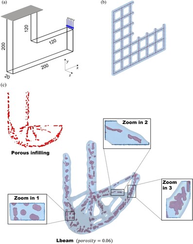
For the multiscale L-beam problem, 228 bar components and 684 sphere components are manipulated to optimise the bio-mimicking porous structure. As Figure 7(b) shows, the initial design is generated with a similar arrangement of bar components as in the MBB case. The cross-section profile of each bar is controlled by 24 polygon vertices. There are three spheres inside each bar at the micro level for the generation of voids. The three spheres are equidistant between two endpoints of bar components. The spheres shown in Figure 7(b) is also overlapped at some locations. The volume target volume fraction and the target porosities are the same as the settings in MBB design, where the $f$ is equal to 0.3 and the porosity $p$ is equal to 0.06, 0.08, and 0.10, respectively.

The two constraints need to reach the target after the optimisation. Figure 7(c) shows the optimised L-beam under the 0.06 porosity constraints. From the observation of the red-highlighted porous infilling shown in Figure 7(c), a certain degree of uniform distribution of voids with stochasticity has been achieved. The morphology of voids is illustrated in the zoom-in parts of Figure 7(c). The typical morphologies in L-beam design are similar to the MBB design, where zoom-in 1 illustrates the spherical voids that are distributed separately, zoom-in 2 illustrates the stripe void that generated form the overlap of several spheres, and the zoom-in 3 illustrates the void cluster that generated form the overlap of large quantities of spheres. Both separate regular voids and irregular voids can be obtained by the proposed method.

Figure 8(a) shows the optimised L-beam with 0.08 and 0.10 porosity constraints. Both optimised designs can achieve the expected pores distribution and the void morphology as the 0.06 porosity design. Figure 8(b) shows the compliance history during the optimisation. Figure 8(c and d) show the volume fraction history and the porosity history. The L-beam with 0.06 porosity constraints (blue curve), 0.08 porosity constraints (red curve), and 0.10 porosity constraints (yellow curve) case can converge after 100 iterations. The volume and porosity constraint targets are achieved for all three optimised designs. The compliance for optimised L-beam with 0.06, 0.08, and 0.10 porosity constraints are 14.36, 13.91, and 14.38, respectively.

Figure 8. Optimisation results of the multiscale bio-mimicking L-beam case: (a) Optimised L-beam with 0.08 and 0.10 porosity, (b) Compliance history, (c) Volume fraction history, (d) Porosity history.

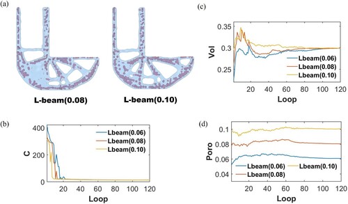
The effectiveness of concurrent multiscale optimisation in the proposed method can be observed from the L-beam under different porosities. As Figure 8(a) shows, the outer shape of the porosity 0.08 case and porosity 0.10 case is obviously different. The outer shape is dependent on the distribution of inner voids.

4.3 Porous simply cubic (SC) lattice structure

To validate the potential application of the proposed bio-mimicking structural optimisation method, the simply cubic (SC) lattice with minimal compliance is designed. As Figure 9(a) shows, the size of the design space is $80\times 80\times 80$. The lattice is under compression from the top plane with the fixation on the bottom plane. To conduct the simulation of compression, the top and the bottom board in grey colour are set to be passive solid, which means they maintain purely solid during the optimisation. The distributed load in the negative $y$-direction is applied to the up surface of the top passive solid board. The degree of freedom is fixed for the nodes on the down surface of the bottom passive solid board.

Figure 9. Simply cubic (SC) lattice problem: (a) The definition of SC lattice problem, (b) Initial design of SC lattice in isometric transparent view, (c) The optimised design of SC lattice with 0.10 porosity.

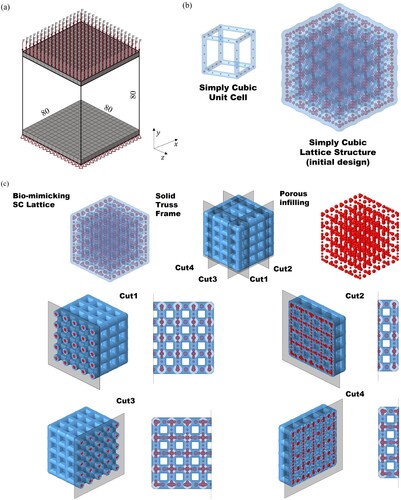
For the SC lattice problem, 300 bar components and 1500 sphere components are manipulated to optimise the bio-mimicking porous structure. As Figure 9(b) shows, the initial design consists of 300 bars to construct a lattice with $4\times 4\times 4$ unit cells. As the top left of Figure 9(b) shows, each unit cell is constructed with 12 bars that locate at cubic edges. There are 5 spheres inside each bar at the micro level for the generation of voids. The spheres are equidistant between two endpoints of bar components. The target porosity $p$, which is the volume ratio of infillings to the solid SC frame, is set to 0.10, 0.15, and 0.20, respectively.

Figure 9(c) shows the optimised SC lattice under the 0.10 porosity constraints, where the voids take 10% volume inside the solid lattice. From the observation of the red porous infilling shown in Figure 9(c), a certain degree of uniform distribution of voids has been achieved. As Figure 9(c) shows, the distribution of the voids is evaluated at four different cutting planes. The cut 1 and cut 3 are in the middle of the truss. Cut 2 and cut 4 are at the joint, which is the region that connects different trusses. As the results illustrated, the voids tend to aggregate in the joint region. The voids in the truss region tend to exist as single big spherical voids. Another observation is that the size of voids inside the vertical truss, which are aligned in the compression direction, is smaller than the voids on the horizontal surface. The reason for the small size of voids in the vertical truss is that stronger trusses are needed under vertical compression.

Figure 10(a and b) show the optimised SC lattice with 0.15 and 0.20 porosity constraints, respectively. From the comparison between three optimised SC lattices, the voids tend to change from separate spherical shape to continuous column shape when the porosity increases. The voids for all three cases prefer to have a large size in the joint region. Figure 10(c) shows the compliance history during the optimisation. Figure 10(d and e) show the volume fraction history and the porosity history. The bio-mimicking SC lattice with 0.10 porosity constraints (blue curve), 0.15 porosity constraints (red curve), and 0.20 porosity constraints (yellow curve) case can converge after 80 iterations. The volume and porosity constraint targets are achieved for all three optimised designs. The compliance for 0.10, 0.15, and 0.20 porosity designs are 0.0422, 0.0457, and 0.0513, respectively. To further investigate the reason behind the distribution of voids, the strain energies at all elements for the pure solid SC under the same compression loads are evaluated. The solid SC lattice is generated by replacing all the voids inside the bio-mimicking SC design with solid material. The solid SC has the same shape as the solid frame as Figure 9(c) shows. The compliance and volume fraction of solid SC under compression are shown with the purple lines in Figure 10(c and d). The compliance of solid SC is 0.0421. With comparison to the solid SC lattice design, the compliance of 0.10 porosity bio-mimicking SC is approximately the same as the solid SC, where the volume has been saved by 10%.

Figure 10. Optimisation results of the simply cubic (SC) lattice case: (a) Optimised SC lattice with 0.15 porosity, (b) Optimised SC lattice with 0.20 porosity, (c) Compliance history, (d) Volume fraction history, (e) Porosity history, (f) Strain energy at all elements for solid SC lattice under compression.

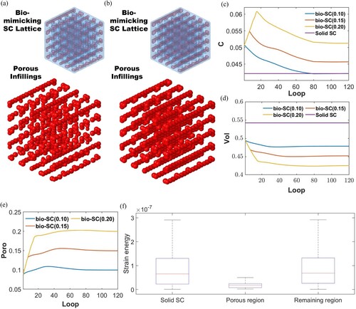
Figure 10(f) shows the strain energy at all elements for the solid SC, porous region, and the remaining region. It should be noticed that the porous region is composed of purely solid elements that are only located at the same positions where the void elements locate in the optimised porosity 0.10 bio-mimicking SC lattice. In Figure 10(f), the red line inside the box represents the median strain energy at the relevant region. The blue box represents the intermediate level of strain energy which is between 25 and 75%. The top and bottom whiskers represent extreme data. The strain energy in the porous region is much smaller than in the remaining region. Because the elements that own lower strain energy have little potential to deform, the porous region is less effective as a support to resist the load. Therefore, the proposed optimisation method tends to eliminate the low-efficient elements to design an effective lightweight structure.

4.4 Porous octet-truss (OT) unit cell structure

To validate the ability to optimise lattice structure at a lower level for the proposed bio-mimicking structural optimisation method, the octet-truss (OT) unit cell with minimal compliance is designed. As Figure 11(a) shows, the size of the design space is $80\times 80\times 80$. The remaining settings are the same as the SC lattice case.

Figure 11. Porous octet-truss (OT) unit cell problem: (a) The definition of OT unit cell problem, (b) Initial design of OT unit cell in isometric transparent view, (c) The optimised design of OT unit cell with 0.06 porosity.

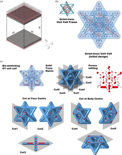
For the OT unit cell problem, 36 bar components and 288 sphere components are manipulated to optimise the bio-mimicking porous structure. As Figure 11(b) shows, the initial design consists of 36 bars to construct the frame of the OT unit cell. There are 24 bars, which are illustrated in cyan colour in the small cube at the top left of Figure 11(b), that connect the vertices of the cube and the face centres of the cube. Another 12 bars in pink colour are utilised to construct an octahedron that connects all face cubic centres. There are 8 spheres inside each bar at the micro level for the generation of voids. The 8 spheres are equidistant between two endpoints of bar components. The target porosity $p$ is set to 0.06, 0.08, and 0.10, respectively.

Figure 11(c) shows the optimised OT unit cell under the 0.06 porosity constraints, where the voids take 6% volume inside the solid unit cell. From the observation of the red porous infilling shown in Figure 11(c), a certain degree of uniform distribution of voids has been achieved. The voids tend to concentrate more at the bottom of the unit cell. As Figure 11(c) shows, the distribution of the voids is evaluated at six different cutting planes. Cut 1 and cut 2 are at the two vertical faces of cubic and cut 3 is at the bottom face of cube. Cut 4 and cut 5 are at the two orthogonal surfaces where the vertical truss in the octahedron locates and cut 6 is at the surface where the horizontal truss in octahedron locates. As the results illustrate, the voids tend to aggregate at the joints that connect trusses as big spheres except for the bottom face of the cube (cut 3). The big voids are mainly at the joints rather than in the middle of the truss due to the stretching of trusses under compression. This is reasonable due to the stretch-dominated nature of the OT lattice. The four joints at the bottom surface of the cube are critical supports of the structure due to the fixation at the bottom and the geometric shape of the OT unit cell. Therefore, the four bottom joints (cut 3) tend to have small voids.

Figure 12(a and b) show the optimised OT unit cell with 0.08 and 0.10 porosity constraints, respectively. From the comparison between three optimised OT unit cell, the distribution of voids tends to obey the same mechanism. The average size of voids tends to increase when the target porosity increases. Figure 12(c) shows the compliance history during the optimisation. Figure 12(d and e) show the volume fraction history and the porosity history. The bio-mimicking OT unit cell with 0.06 porosity constraints (blue curve), 0.08 porosity constraints (red curve), and 0.10 porosity constraints (yellow curve) case can converge after 100 iterations. The volume and porosity constraint targets are achieved for all three optimised designs. The compliance for 0.06, 0.08, and 0.10 porosity designs are 0.170, 0.173, and 0.177, respectively. To further investigate the reason behind the distribution of voids, the strain energies at all elements for the pure solid OT unit cell under the same compression loads are evaluated. The solid OT unit cell is generated by eliminating all the voids in the bio-mimicking OT design. The solid SC has the same shape as the solid frame as Figure 11(c) shows. The compliance and volume fraction of solid OT under compression are shown with the purple lines in Figure 12(c and d). The compliance of solid OT is 0.179. In comparison to the solid OT, the compliance of all bio-mimicking OT can beat the solid OT according to the lower compliance.

Figure 12. Optimisation results of the octet-truss (OT) unit cell case: (a) Optimised OT unit cell with 0.08 porosity, (b) Optimised OT unit cell with 0.10 porosity, (c) Compliance history, (d) Volume fraction history, (e) Porosity history, (f) Strain energy at all elements for solid OT unit cell under compression.

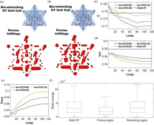
Figure 12(f) shows the strain at all elements for the solid OT, porous region, and the remaining region. It should be noticed that the porous region is composed of purely solid elements that are only located at the same positions where the void elements locate in the optimised porosity 0.06 bio-mimicking OT unit cell. In Figure 12(f), the red line inside the box represents the mean strain energy at the relevant region. The blue box represents the intermediate level of strain energy that is between 25% and 75%. The top and bottom whiskers represent extreme data. Similarly, the low-efficient elements in the porous region, which have lower strain energy under loading, have been eliminated to design an effective lightweight structure.

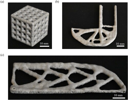
5. 3d printing validation and characterisation

In this section, the manufacturability of optimised designs from the proposed approach is validated by the SLM fabrication and the following observations with micro-CT. The optimised porous MBB with 0.10 porosity constraint, the L-beam with 0.10 porosity constraint, and the SC lattice with 0.20 porosity constraint were selected as validation samples. These samples were then examined by micro-CT for overall shape and porosity check. For the validation part, the MBB and L-beam samples are scaled down to 32% of the design dimension in Figure 5(a) and Figure 7(a), respectively. The SC lattice is scaled down to 40% of the design dimension in Figure 9(a).

Prior to fabrication, the build job was prepared in Magics software (Materialise, Belgium) where support structure was generated as needed and drain holes were introduced to the CAD models in order to remove the entrapped powder after fabrication. These holes were 500 µm in diameter. This approach is adopted when fabricating components with enclosed volumes and proves to have negligible effect on the mechanical behaviour (Crook et al. 2020). All the samples were fabricated with the EOS M270 machine equipped with a 200 W laser and scan speed up to 7 m/s. Gas atomised AlSi10Mg powder, which has a mean diameter of 11 µm ranging from 4 to 34 µm, was utilised to fabricate all samples. The layer thickness was set to 20 µm and scanning direction was rotated by 90° between successive layers. After fabrication, samples were removed from the building plate using CUT 30P-AgieCharmilles Wire Electric Discharge Machine. Support was then manually removed and the samples were post processed by shot-peening to remove residual powder adhering to the outer surfaces. The fabricated samples are shown in Figure 13.

Figure 13. The AlSi10Mg samples fabricated by SLM: (a) Optimised simply cubic (SC) lattice with 0.20 porosity, (b) Optimised L-beam with 0.10 porosity, (c) Optimised Messershmitt-Bolkow-Blohm (MBB) with 0.10 porosity.

The features of all samples were examined by using the Bruker SkyScan 1275 x-ray micro-CT machine. The filter for micro-CT was Cu with 1 mm thickness. The scanning was conducted among 360° with a rotation step size of 0.5°. The scanning slices were reconstructed using nRecon software (Bruker Pty Ltd.). In order to conduct the quantitative analysis of the cross-sectional features, the reconstructed images were transformed into the binary form using the CTAn software (Bruker Pty Ltd.). The results for the MBB, the L-beam and the SC lattice are shown in Figures 14–16, respectively.

Figure 14. The micro-CT results of Messershmitt-Bolkow-Blohm (MBB) with 0.10 porosity: (a) As-designed 3D model, (b) Reconstructed 3D model of the as-manufactured sample via micro-CT, (c) Cross-section view of reconstructed micro-CT 3D model from the as-manufactured sample at $zx$-plane, (d) 2D cross-section slice of the as-designed model at $zx$-plane, (e) 2D cross-section micro-CT slice of as-manufactured sample at $zx$-plane.

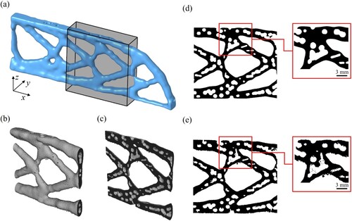
Figure 15. The micro-CT results of L-beam with 0.10 porosity: (a) As-designed 3D model, (b) Reconstructed 3D model of as-manufactured sample via micro-CT, (c) Cross-section view of the reconstructed micro-CT 3D model from the as-manufactured sample at $yz$-plane, (d) 2D cross-section slice of the as-designed model at $yz$-plane, (e) 2D cross-section micro-CT slice of the as-manufactured sample at $yz$-plane.

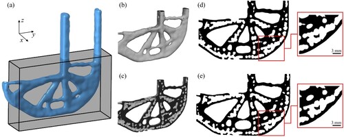
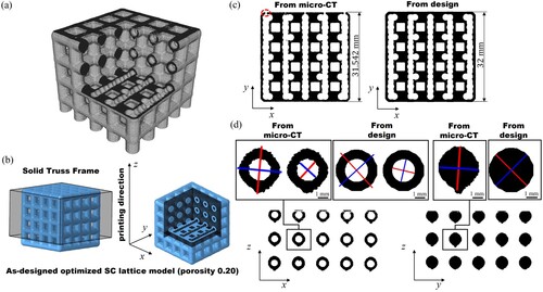
Figure 16. The micro-CT results of simply cubic (SC) lattice with 0.20 porosity: (a) Reconstructed 3D model of the as-manufactured sample via micro-CT, (b) As-designed 3D model, (c) 2D cross-section micro-CT slice of the as-manufactured sample and 2D cross-section slice of the as-designed model at $xy$-plane, (d) 2D cross-section micro-CT slice of the as-manufactured sample at $zx$-plane and $yz$-plane.

Due to the limitations on the scanning dimensions of the micro-CT machine, as Figure 14(a) shown, only part of the sample inside the grey box was scanned for validation. The 3D reconstructed model from micro-CT is shown in Figure 14(b and c). From the observation of the reconstructed 3D model, the overall shape of the as-manufactured MBB sample has negligible deviations from the as-designed model. To further examine the manufacturing quality of inner pores, the 2D slices from the cutting at the $zx$-plane were generated from both micro-CT images and the as-designed model. The 2D slice from micro-CT is shown in Figure 14(e). In the comparison to the slice from the as-designed model which is (shown in Figure 14(d)), both the inner pores and the outer shape of the solid truss are impacted by the overhang. The detailed features of the as-designed slice and the as-manufactured slice are shown in the zoom-in of Figures 14(d and e). From the observations, the features of the as-designed model are well fabricated. Although the overhang has impacts, the bio-mimicking MBB is feasible for manufacturing with admissible quality.

Due to the scanning limitations, as Figure 15(a) shows, only part of the sample inside the grey box was scanned for validation. The 3D reconstructed model from micro-CT is shown in Figure 15(b and c). From the observation of the reconstructed 3D model, the overall shape of as-manufactured L-beam sample has negligible deviations compared with the as-designed model. The 2D slices from the cutting at the $yz$-plane were generated from both micro-CT images and the as-designed model. The 2D slices from the micro-CT and the as-designed model are shown in Figure 15(e and d), respectively. Similar to the MBB case, the overhang issues can be observed from comparison. The detailed features of the as-designed slice and the as-manufactured slice are shown in the zoom-in of Figure 15(d and e). The features of the as-designed model are well fabricated.

From the MBB and L-beam cases, the proposed approach has been validated to be feasible with manufacturability. In order to further investigate the manufacturing quality, a quantitative analysis has been conducted on the SC lattice case with processing on micro-CT data. Due to the scanning limitations, as Figure 16(b) shown, only part of the sample inside the grey box was scanned for validation. The 3D reconstructed model from micro-CT is shown in Figure 16(a). The inner features of the as-designed model are shown in Figure 16(b). As Figure 16(c) shows, the near-column shape hollow features at the $xy$-plane are well fabricated. The length of the cube for the as-manufactured sample and the as-designed model is 31.542 and 32 mm, respectively. The small cuttings, which are shown inside the red dashed circle in Figure 16(c), are facilitated at the outer surface of samples to assist in the removal of residual adhesive powders.

As Figure 16(d) shows, the near-circular shape cross-section features are existed at $zx$- and $yz$-plane. To facilitate quantitative analysis, the MATLAB code was applied to extract the region properties on both the solid cross-section at $zx$-plane and the hollow ring-shape cross-section at $yz$-plane. The region properties are based on the construction of an ellipse that has the same second moments as the region represented in pixels. As the zoom-in of Figure 16(d) shows, the major axes of constructed ellipses are shown in red colour. The minor axes of constructed ellipses are shown in blue colour.

For the as-manufactured ring-shape cross-section from micro-CT at $zx$-plane, the major axes length of the outer profile and inner profile are 4.516 and 2.070 mm. The minor axes length of the outer profile and inner profile are 4.185 and 2.000 mm. For the as-designed counterpart, the major axes length of the outer profile and inner profile are 4.540 and 2.201 mm. The minor axes length of the outer profile and inner profile are 4.531 and 2.197 mm. For the evaluation of shape, the ratio of major length to minor length is calculated. For the outer profile, the ratios for the as-manufactured case and as-designed counterpart are 1.079 and 1.002, respectively. For the inner profile, the ratios for the as-manufactured case and as-designed counterpart are 1.035 and 1.002, respectively. The average diameters of the cross-section are calculated as the average of major length and minor length to evaluate the size. For the outer profile, the average diameters for the as-manufactured case and as-designed counterpart are 4.350 and 4.536 mm. For the inner profile, the average diameters for the as-manufactured case and as-designed counterpart are 2.035 and 2.199 mm.

As a result, the as-deigned cross-section is in perfect circular shape. The shape deviation for the as-manufactured outer and inner profiles are 3.5 and 8%, respectively. More shape deviations have been induced by the manufacturing process for the outer profile than the inner profile. As Figure 16(d) shows, the shape deviation is due to the overhang along the printing direction. More overhangs are observed in the outer profile than the overhangs in the inner profile, showing that the outer profile can provide good support for the fabrication of inner hollow features. The size deviations of the outer and inner sections are 4.1 and 7.4%, respectively.

For the as-manufactured solid cross-section from the micro-CT at $yz$-plane, the major axis length of the profile is 4.116 mm. The minor axis length of the profile is 3.668 mm. For the as-designed counterpart, the major axis length of the profile is 3.970 mm. The minor axes length of the profile is 3.962 mm. The ratios of major length to minor length for the as-manufactured case and as-designed counterpart are 1.122 and 1.002, respectively. The average diameters for the as-manufactured case and as-designed counterpart are 3.892 and 3.966 mm. As a result, the shape deviation for as-manufactured profile is 12.2%. The size deviation of profile is 1.8%. From the comparison between the hollow ring-shape cross-section and the solid circular-shape cross-section, the solid truss tends to have more shape deviation. The truss with hollow sections tends to have more size deviation. The shape and size deviations at both solid cross-section and hollow cross-section show the admissible manufacturing quality of the proposed approach.

The information of pore size is illustrated in the Table 1. The examination is from the reconstructed micro-CT model. The middle section of MBB with 0.10 porosity (shown in Figure 14(c)) and the bottom section of L-beam with 0.10 porosity (shown in Figure 15(c)) are examined to provide pore size analysis. For both cases, the existence of pores with small size (0.5−1 mm³), medium size (1−10 mm³), and large size (>10 mm³) demonstrates the capability of generating uniform distributed pores in the proposed approach. In addition, different size of pores show that sphere components can work independently (pores in small size) or collaborate as small clusters (pores in medium size) and large clusters (pores in large size). With comparison to the solid frame, the volume of the largest pore, which is equal to 74 mm³ in the MBB case and 24 mm³ in the L-beam case, is below 2% of the volume of the solid frame, showing the clear scale separation and the good multiscale design abilities of the proposed approach.

Table 1. Pore size information of reconstructed model from micro-CT.

Sample	Evaluated section	Volume of structure	Pore size
L-beam	Bottom part (model shown in Figure 15(c))	Total volume: 3471 mm^3 Volume of pores: 247 mm^3 Volume of solid frame: 3224 mm^3	Number of pores: Total: 161 0.5 mm^3 < Volume < 1 mm^3: 133 1 mm^3 ≤ Volume < 10 mm^3: 25 10 mm^3 ≤ Volume < 74 mm^3: 3
MBB	Middle part (model shown in Figure 14(c))	Total volume: 1860 mm^3 Volume of pores: 205 mm^3 Volume of solid frame: 1655 mm^3	Number of pores: Total: 49 0.5 mm^3 < Volume < 1 mm^3: 23 1 mm^3 ≤ Volume < 10 mm^3: 17 10 mm^3 ≤ Volume < 24 mm^3: 9

6. Conclusion

In this work, we proposed a discrete component-based concurrent multiscale optimisation approach for the truss-like structure at the macro level and the bio-mimicking porous structure at the micro level. For the numerical validation section, classical beam examples, lattice structure design, and unit cell design were illustrated to confirm the effectiveness and functionalities of the proposed approach. In addition, the MBB beam, L-beam, and SC lattice samples were fabricated by SLM technology and then evaluated with the micro-CT technique. The following conclusions are made:

• The explicit description of geometric components provides the strong capabilities of ensuring geometric features. The overlapping, moving, and morphing of bar components provide the ability to generate flexible structural shapes at the macro-level.

• The porous infillings can be ensured by the proposed approach. Inspired by the turtle carapace, the bar components are separated into shell and core regions. The sphere components can move, overlap, and resize inside the related bar in the local coordinate system to sufficiently generate both the regular and irregular porous infillings.

• The effective balance between uniform and stochastic pores distribution and porosity control were observed to validate the effectiveness of bio-mimicking functionalities. The outer truss-like shapes of optimised beams show the correctness of the proposed approach.

• The proposed approach has abilities to optimise lattice structure at truss-level and single unit cell level are demonstrated. From the numerical result, the optimised SC lattice and OT unit cell with 0.10 porosity have larger stiffness than the solid SC lattice.

• The admissible manufacturability of the proposed approach has been demonstrated. From the observations of as-manufactured samples via micro-CT, the shape and size of features can be well fabricated.

The proposed approach can generate porous infillings with numerical-based optimisation guidance. In the future, the findings of this research may be explored further, especially for anisotropy control and energy absorption applications.

Acknowledgment

The authors would like to thank RMIT Microscopy and Microanalysis Facility (RMMF) for the access to X-ray micro-computed tomography facility. This research was partially carried out using the Core Technology Platforms resources at New York University Abu Dhabi.

Disclosure statement

No potential conflict of interest was reported by the author(s).

Additional information

Funding

This work was supported by Vingroup Innovation Foundation (VINIF): [Grant Number VINIF.2019.DA04].

References

- Achrai, B., and H. D. Wagner. 2017. “The Turtle Carapace as an Optimized Multi-Scale Biological Composite Armor–A Review.” Journal of the Mechanical Behavior of Biomedical Materials 73: 50–67.
- Afshar, M., A. P. Anaraki, and H. Montazerian. 2018. “Compressive Characteristics of Radially Graded Porosity Scaffolds Architectured with Minimal Surfaces.” Materials Science and Engineering: C 92: 254–267.
- Alberdi, R., R. Dingreville, J. Robbins, T. Walsh, B. C. White, B. Jared, and B. L. Boyce. 2020. “Multi-morphology Lattices Lead to Improved Plastic Energy Absorption.” Materials & Design 194: 108883.
- Alomar, Z., and F. Concli. 2021. “Compressive Behavior Assessment of a Newly Developed Circular Cell-Based Lattice Structure.” Materials & Design 205: 109716.
- Bai, J., and W. Zuo. 2020. “Hollow Structural Design in Topology Optimization via Moving Morphable Component Method.” Structural and Multidisciplinary Optimization 61 (1): 187–205.
- Bendsøe, M. P. 1989. “Optimal Shape Design as a Material Distribution Problem.” Structural Optimization 1 (4): 193–202.
- Bendsøe, M. P., and N. Kikuchi. 1988. “Generating Optimal Topologies in Structural Design Using a Homogenization Method.” Computer Methods in Applied Mechanics and Engineering 71 (2): 197–224.
- Bose, S., N. Sarkar, and D. Banerjee. 2021. “Natural Medicine Delivery from Biomedical Devices to Treat Bone Disorders: A Review.” Acta Biomaterialia 126: 63–91.
- Buhl, T., C. B. Pedersen, and O. Sigmund. 2000. “Stiffness Design of Geometrically Nonlinear Structures Using Topology Optimization.” Structural and Multidisciplinary Optimization 19 (2): 93–104.
- Clausen, A., N. Aage, and O. Sigmund. 2016. “Exploiting Additive Manufacturing Infill in Topology Optimization for Improved Buckling Load.” Engineering 2 (2): 250–257.
- Crook, C., J. Bauer, A. Guell Izard, C. S. de Oliveira, J. M. de Souza e Silva, J. B. Berger, and L. Valdevit. 2020. “Plate-nanolattices at the Theoretical Limit of Stiffness and Strength.” Nature Communications 11 (1): 1–11.
- Du Plessis, A., C. Broeckhoven, I. Yadroitsava, I. Yadroitsev, C. H. Hands, R. Kunju, and D. Bhate. 2019. “Beautiful and Functional: A Review of Biomimetic Design in Additive Manufacturing.” Additive Manufacturing 27: 408–427.
- Gao, X., and H. Ma. 2015. “Topology Optimization of Continuum Structures Under Buckling Constraints.” Computers & Structures 157: 142–152.
- Gautam, R., S. Idapalapati, and S. Feih. 2018. “Printing and Characterisation of Kagome Lattice Structures by Fused Deposition Modelling.” Materials & Design 137: 266–275.
- Ghannadpour, S., M. Mahmoudi, and K. H. Nedjad. 2022. “Structural Behavior of 3D-Printed Sandwich Beams with Strut-Based Lattice Core: Experimental and Numerical Study.” Composite Structures 281: 115113.
- Ghazlan, A., T. Ngo, P. Tan, Y. M. Xie, P. Tran, and M. Donough. 2021. “Inspiration from Nature's Body Armours–A Review of Biological and Bioinspired Composites.” Composites Part B: Engineering 205: 108513.
- Guo, X., W. Zhang, and W. Zhong. 2014. “Doing Topology Optimization Explicitly and Geometrically—a new Moving Morphable Components Based Framework.” Journal of Applied Mechanics 81 (8): 081009.
- Hoang, V.N., N.L. Nguyen, P. Tran, M. Qian, and H. Nguyen-Xuan. 2020a. “Adaptive Concurrent Topology Optimization of Cellular Composites for Additive Manufacturing.” JOM Journal of the Minerals Metals and Materials Society 72 (6): 2378–2390.
- Hoang, V.-N., P. Tran, N.L. Nguyen, K. Hackl, and H. Nguyen-Xuan. 2020b. “Adaptive Concurrent Topology Optimization of Coated Structures with Nonperiodic Infill for Additive Manufacturing.” Computer-Aided Design 129: 102918.
- Hoang, V.-N., P. Tran, V. T. Vu, and H. Nguyen-Xuan. 2020c. “Design of Lattice Structures with Direct Multiscale Topology Optimization.” Composite Structures 252: 112718.
- Hoang, V.-N., and H. Nguyen-Xuan. 2020. “Extruded-geometric-component-based 3D Topology Optimization.” Computer Methods in Applied Mechanics and Engineering 371: 113293.
- Holmberg, E., B. Torstenfelt, and A. Klarbring. 2013. “Stress Constrained Topology Optimization.” Structural and Multidisciplinary Optimization 48 (1): 33–47.
- Kadkhodapour, J., H. Montazerian, and S. Raeisi. 2014. “Investigating Internal Architecture Effect in Plastic Deformation and Failure for TPMS-Based Scaffolds Using Simulation Methods and Experimental Procedure.” Materials Science and Engineering: C 43: 587–597.
- Kumar, T., and K. Suresh. 2020. “A Density-and-Strain-Based K-Clustering Approach to Microstructural Topology Optimization.” Structural and Multidisciplinary Optimization 61 (4): 1399–1415.
- Lan, T., and P. Tran. 2021. “Multiscale Topology Optimization of Lattice Structure Using 3D Moving Hollow Morphable Bars.” JOM Journal of the Minerals Metals and Materials Society 73 (12): 4141–4153.
- Lee, J., C. Kwon, J. Yoo, S. Min, T. Nomura, and E. M. Dede. 2021. “Design of Spatially-Varying Orthotropic Infill Structures Using Multiscale Topology Optimization and Explicit de-Homogenization.” Additive Manufacturing 40: 101920.
- Liu, F., T. Zhou, T. Zhang, H. Xie, Y. Tang, and P. Zhang. 2022. “Shell Offset Enhances Mechanical and Energy Absorption Properties of SLM-Made Lattices with Controllable Separated Voids.” Materials & Design 217: 110630.
- Liu, P., Z. Kang, and Y. Luo. 2020. “Two-scale Concurrent Topology Optimization of Lattice Structures with Connectable Microstructures.” Additive Manufacturing 36: 101427.
- Peng, C., K. Fox, M. Qian, H. Nguyen-Xuan, and P. Tran. 2021. “3D Printed Sandwich Beams with Bioinspired Cores: Mechanical Performance and Modelling.” Thin-Walled Structures 161: 107471.
- Peng, C., and P. Tran. 2020. “Bioinspired Functionally Graded Gyroid Sandwich Panel Subjected to Impulsive Loadings.” Composites Part B: Engineering 188: 107773.
- Peng, C., P. Tran, and A. P. Mouritz. 2022. “Compression and Buckling Analysis of 3D Printed Carbon Fibre-Reinforced Polymer Cellular Composite Structures.” Composite Structures, 116167.
- Ravari, M.K., M. Kadkhodaei, M. Badrossamay, and R. Rezaei 2014. “Numerical Investigation on Mechanical Properties of Cellular Lattice Structures Fabricated by Fused Deposition Modeling.” International Journal of Mechanical Sciences 88: 154–161.
- Sanders, E., A. Pereira, and G. Paulino. 2021. “Optimal and Continuous Multilattice Embedding.” Science Advances 7 (16): eabf4838.
- Sharma, D., and S. S. Hiremath. 2022. “Bio-inspired Repeatable Lattice Structures for Energy Absorption: Experimental and Finite Element Study.” Composite Structures 283: 115102.
- Shen, J., Y. M. Xie, X. Huang, S. Zhou, and D. Ruan. 2012. “Mechanical Properties of Luffa Sponge.” Journal of the Mechanical Behavior of Biomedical Materials 15: 141–152.
- Tee, Y. L., and P. Tran. 2021. “On Bioinspired 4d Printing: Materials, Design and Potential Applications.” Australian Journal of Mechanical Engineering 19 (5): 642–652.
- Thielen, M., C. N. Z. Schmitt, S. Eckert, T. Speck, and R. Seidel. 2013. “Structure–Function Relationship of the Foam-Like Pomelo Peel (Citrus Maxima)—an Inspiration for the Development of Biomimetic Damping Materials with High Energy Dissipation.” Bioinspiration & Biomimetics 8 (2): 025001.
- Tran, P., T. D. Ngo, A. Ghazlan, and D. Hui. 2017. “Bimaterial 3D Printing and Numerical Analysis of bio-Inspired Composite Structures Under in-Plane and Transverse Loadings.” Composites Part B: Engineering 108: 210–223.
- Wang, C., X. Gu, J. Zhu, H. Zhou, S. Li, W. Zhang. 2020. “Concurrent Design of Hierarchical Structures with Three-Dimensional Parameterized Lattice Microstructures for Additive Manufacturing.” Structural and Multidisciplinary Optimization 61 (3): 869–894.
- Wang, C., Z. Zhao, M. Zhou, O. Sigmund, and X. S. Zhang. 2021. “A Comprehensive Review of Educational Articles on Structural and Multidisciplinary Optimization.” Structural and Multidisciplinary Optimization 64 (5): 2827–2880.
- Wang, M. Y., X. Wang, and D. Guo. 2003. “A Level set Method for Structural Topology Optimization.” Computer Methods in Applied Mechanics and Engineering 192 (1-2): 227–246.
- White, B. C., A. Garland, R. Alberdi, and B. L. Boyce. 2021. “Interpenetrating Lattices with Enhanced Mechanical Functionality.” Additive Manufacturing 38: 101741.
- Wickramasinghe, S., T. Do, and P. Tran. 2020. “FDM-based 3D Printing of Polymer and Associated Composite: A Review on Mechanical Properties, Defects and Treatments.” Polymers 12 (7): 1529.
- Xiao, Z., Y. Yang, R. Xiao, Y. Bai, C. Song, and D. Wang 2018. “Evaluation of Topology-Optimized Lattice Structures Manufactured via Selective Laser Melting.” Materials & Design 143: 27–37.
- Xie, Y. M., and G. P. Steven. 1993. “A Simple Evolutionary Procedure for Structural Optimization.” Computers & Structures 49 (5): 885–896.
- Yang, W., and J. McKittrick. 2013. “Separating the Influence of the Cortex and Foam on the Mechanical Properties of Porcupine Quills.” Acta Biomaterialia 9 (11): 9065–9074.
- Zhang, W., D. Li, J. Yuan, J. Song, and X. Guo. 2017. “A new Three-Dimensional Topology Optimization Method Based on Moving Morphable Components (MMCs).” Computational Mechanics 59 (4): 647–665.
- X. Xiang, W. Jin, C. Tengteng, W. H. Chun 2018. “Crushing Analysis for Novel bio-Inspired Hierarchical Circular Structures Subjected to Axial Load.” International Journal of Mechanical Sciences 140: 407–431.
- Zhang, W., Y. Sha, T.X. Yu, and X. Jun 2019. “Crushing Resistance and Energy Absorption of Pomelo Peel Inspired Hierarchical Honeycomb.” International Journal of Impact Engineering 125: 163–172.
- Zhao, Y., V. N. Hoang, G.W. Jang, and W. Zuo. 2021. “Hollow Structural Topology Optimization to Improve Manufacturability Using Three-Dimensional Moving Morphable Bars.” Advances in Engineering Software 152: 102955.