A novel multiscale process simulation to predict the impact of intrinsic heat treatment on local microstructure gradients and bulk hardness of AISI 4140 manufactured by laser powder bed fusion

ABSTRACT

Although finite element model based process simulations for the laser powder bed fusion additive manufacturing process have become more common in the recent years, the proposed approaches are often only viable for materials without complex phase transformations. Process simulations for materials such as the quench and tempering steel AISI 4140 typically lead to higher computational cost due to the finer mesh and time steps needed for more complex material models. This study proposes a novel multiscale approach to combine the advantages of the macroscale and mesoscale models into one framework, in order to reduce computational cost while retaining the high accuracy. The implementation of these multiscale methods was validated by experimentally analyzing multiple parameter combinations regarding bulk hardness and local microstructure differences. The results show an accurate prediction of bulk hardness and localised tempering effects while reducing the computational cost in order to simulate the component scale.

KEYWORDS:

• Laser powder bed fusion
• additive manufacturing
• quench and tempering steel
• multiscale finite element simulation
• hardness

1. Introduction

Laser-based powder bed fusion (PBF-LB) has become one of the standard processes for metal additive manufacturing (AM), especially for steels. Due to the freedom of design, relatively new approaches such as topology optimisation can be used to their full potential. While most of the commercially available steel powders contain only low amounts of carbon, steels with higher carbon content such as AISI 4140 have become more common in recent years. These steels are more challenging to print due to the martensitic transformation during cooling, which leads to high local stresses and increases the risk of cold cracking associated with the respective volume change during transformation. The negative effects of a higher carbon content regarding the cold cracking risk were analysed by Hearn and Eduard [1]. Most research on additively manufactured carbon steels is focused on defect-free AM reducing the porosity [2–5] and cracks [1,3,4], as well as static mechanical properties [3,5,6].

In conventional manufacturing, the quench and tempering (Q&T) steel AISI 4140 is often used because of its wide range of mechanical properties, adjustable through different heat treatment methods. The most common processes for surface hardening of Q&T steels include laser- and induction-hardening [7–10]. With the PBF-LB process, the variation of process parameters can lead to significant changes in microstructure and hardness [3]. Thus, a functionally graded material state, similar to the one after induction hardening, could be created directly within the printing process. The understanding of the effects of process parameter variation is therefore of great interest in current research. Damon et al. [3] reported a decrease in resulting bulk hardness of 100 HV1 for printing AISI 4140 while increasing the energy density from $70\mathrm{J}{\mathrm{m}\mathrm{m}}^{-3}$ to $225\mathrm{J}{\mathrm{m}\mathrm{m}}^{-3}$. Further studies on intrinsic heat treatment effects were conducted during the PBF-LB printing process for martensitic stainless steel [11] and maraging steel [12–14]. Hearn et al. [15] studied the intrinsic heat treatment effect for a Fe-0.45C martensitic steel similar to the AISI 4140 used in this study. They analysed the tempering states after the process by scanning electron microscopy, transmission electron microscopy and atom probe tomography. Their findings indicate that tempering during the PBF-LB process induces the precipitation of nanosized cementite at previously carbon-enriched boundaries, which noticeably reduces the hardness of martensite. They also observed a decrease in hardness by increasing the volume energy density (VED), which is equivalent to increasing tempering temperature in the conventional process by about 100 K. As these studies prove the theoretical viability of creating a functionally graded part during the printing process, the optimisation and interaction of multiple process parameter combinations in one part can be arduous to do by trial-and-error. Multiple studies on simulating the temperature profile during PBF-LB printing were conducted on the macroscale [16–18], the mesoscale [19–23], or on the microscale of the melt pool, including fluid dynamic simulations [24,25]. Due to the high computational cost, mesoscale and microscale simulations are only possible for small fractions of AM parts. While macroscale simulations can reduce the problem of computational cost, the simplifications applied in these studies, such as combining multiple lines and layers into one approximated energy input, may work for materials like 316L or aluminium alloys. However, these methods lack the thermal accuracy needed for the phase transformations that occur during the processing of martensitic steels. Gh Ghanbari et al. [26] used a multiscale model to simulate the PBF-LB process in 2D. While this method is suitable for the thin walled structures they used, a 3D model is needed in order to simulate the complex thermal history while printing more complex parts. Bresson et al. [27] used a sequential multiscale approach, increasing the accuracy for each simulation level. While this approach can significantly save computational cost with the used Ti-6Al-4V, the differentiation of specific levels will be challenging for materials with more complex phase transformations and tempering behaviour. All these studies confirm the possibility of multiscale simulation models to effectively reduce the computational cost with only a minimal reduction in simulation accuracy.

The objective of this research is to develop a comprehensive simulation framework for martensitic steels, integrating macroscale models with mesoscale models into a unified simulation model. By merging the superior accuracy of the mesoscale with the reduced computational cost of the macroscale, this approach enables the simulation of complex materials at the component level. The multiscale simulation framework will be experimentally validated for single parameter prints, by directly comparing the simulation results for the bulk hardness and localised microstructure predictions with the experimental results. The outcomes of this investigation will enhance the characterisation of martensite tempering in the context of PBF-LB, aiming to enhance the efficiency of single and multi-parameter printing strategies and elucidate the correlation between tempering states and various combinations of process parameters.

2. Material and methods

2.1. Material

Pre-alloyed, inert gas atomised, spherical AISI 4140 (german grade 42CrMo4) powder supplied by Rosswag Engineering GmbH was used for this study. The particle size distribution of the powder, measured by Rosswag Engineering GmbH, had a median of $34\text{μ}\mathrm{m}$, as well as d10 and d90 values of respectively $21\text{μ}\mathrm{m}$ and $56\text{μ}\mathrm{m}$. The chemical composition of the powder and the as-built parts is listed in Table 1.

Table 1. Chemical composition of the powder and the as-built parts in wt.%.

	C	Si	Mn	Cr	Mo	Fe
Powder	0.39	0.25	0.67	1.1	0.24	bal.
As-built	0.39	0.29	0.69	1.06	0.24	bal.

2.2. Samples and process development

Simple cubes with an edge length of 5 mm were manufactured on an SLM280 machine (SLM Solutions Group AG, Germany) by Rosswag Engineering GmbH. The state of the art bidirectional hatching scan strategy was used with an Yb:YAG fiber laser featuring a maximum beam power of 400 W and a focus diameter of $80\text{μ}\mathrm{m}$ at a wave length of 1030 nm. An Ar atmosphere was used to reduce oxidation effects. A fixed layer height t of 0.03 mm was used for this study. In order to find a stable process window, the hatch distance d was varied from 0.1 mm to 0.14 mm, the laser power P from 100 W to 300 W, and the scan speed v from $400\mathrm{m}\mathrm{m}{\mathrm{s}}^{-1}$ to $1100\mathrm{m}\mathrm{m}{\mathrm{s}}^{-1}$. The VED was used for the characterisation of both the experiment and simulation. (1) $VED=\frac{P}{v\cdot d\cdot t}$(1) For the modelling of the material properties 10 mm long cylindrical specimens with an outer diameter of 4 mm and an inner diameter of 3 mm were machined out of printed cylinders.

2.3. Experimental methods

For porosity measurements, nine polished micrograph images parallel to the build direction were captured with a light microscope (Aristomet, Leica Microsystems GmbH), binarised and evaluated using the analyse particles feature included in the image analysis software ImageJ/Fiji [28]. Microstructural analysis has been carried out using a scanning electron microscopy SEM (Leo 50, Carl Zeiss AG) with an acceleration voltage of 10 kV and an inlens detector to investigate the etched cross sections. The samples were therefore etched with a 1% nital etchant (1% nitric acid with 99% ethanol) for 3 s. To investigate the bulk hardness, Vickers hardness tests with a force of 1 kg were carried out (Qness Q30a+, ATM Qness GmbH). A dilatometer (DIL 805, TA Instruments) was used for the heat treatment process, in order to determine the necessary material properties. The FEM simulations were conducted on a workstation with two server type AMD EPYC 7402 24-core processors and 256 GB of RAM. The commercial FEM solver Abaqus/Standard (implicit) was used in combination with Python to automate the workflow for the numerical simulation.

2.4. Numerical simulation

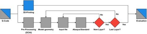
In order to utilise the full potential of the proposed multiscale simulation approach an automated simulation workflow was created to combine the pre-processing, the model creation and FEM calculation steps into one process Figure 1. The simulation is fully automated and starts with the G-Code, which is also used for the printing of the actual parts. The pre-processing workflow consists of the G-Code creation as well as the Python based G-Code analyzer and interpreter (GCAI, See Section 2.4.2). The timing, position and power settings gained from the GCAI module is forwarded to the Abaqus based simulation module. In order to reduce the length of a single simulation, each layer is divided into multiple sub-simulations which include approximately 10 laser lines each. These simulations are restarted with the same model geometry and only need small modifications to the input file (Figure 1, first red decision point). Due to the limitations of the Abaqus software, the simulation module is based on a step-wise approach in order to accommodate the growing geometry of the printed parts. Therefore the current simulation is stopped and a new model geometry is automatically created. The results of the old simulation are then interpolated to the new mesh, the added material is initialised and the next Abaqus simulation is started (Figure 1, second red decision point). This step is needed every time the recoater adds new material to the system. Both decision points were controlled by the current and future positioning of the laser, analysed by the GCAI module from the G-Code file.

Figure 1. Flowchart for the proposed numerical FEM simulation including the experimental route (top) and the simulation route (bottom).

2.4.1. Multiscale simulation approach

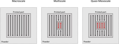
For this study a unique multiscale approach is used to combine the state of the art macroscale and mesoscale approaches in one continuous simulation model Figure 2. The aim of this new approach is to minimise unnecessary computational cost while providing a high quality thermal simulation of a full scale part during printing. For a high quality prediction of the temperature profile and consequently the material properties in the region of interest (ROI), the near- and far-field accuracy of the Goldak heat source (mesoscale, see Section 2.4.9) is combined with the far-field accuracy of the line equivalent heat source model (macroscale, see Section 2.4.9). This approach sacrifices the near-field accuracy in areas that are far enough outside of the ROI. In order to verify the improvements in efficiency and accuracy, a full macroscale model and a quasi-mesoscale model (multiscale model with an ROI doubled in size) were used as well. It can be noted that a mesoscale approach could not be computed for multiple layers due to the extensive computational cost, even for a relatively small sample like the cubes used for this study. In order to compare the multiscale approach used for this study with a theoretically more accurate simulation, a multiscale model with an extensively large ROI was created (quasi-mesoscale model). This quasi-mesoscale model reduces the computational cost compared to a complete mesoscale model, while increasing the accuracy compared to the smaller size ROI used for the other simulations. The simulation workflow and all the material models used for this study will be further explained in the following sections.

2.4.2. Pre-processing: G-Code analyzer and interpreter GCAI

The G-Code analyzer is a Python based script which takes the G-Code file as an input and converts it into a usable format for the Abaqus FEM simulation. Therefore, the script extracts the laser position, laser spot diameter and laser power in dependency of the current simulation time and layer. This data is used in the thermal simulation to create the laser movement and the actual energy input with the two optic models.

Figure 2. Visualisation of the macroscale (left), combined multiscale (middle) and combined quasi-mesoscale (right) simulation approaches. The macroscale (line equivalent heat source) and mesoscale (Goldak heat source) scan paths are represented by arrows. The powder bed is shown in light grey, the macroscale zone in grey and the mesoscale zone in dark grey.

2.4.3. Simulation module: model geometry

The creation of the model geometry including the meshing and input file generation is automated by a Python script using the Abaqus Python Scripting interface for Abaqus/CAE. Following assumptions were integrated into this model geometry in order to simplify the simulation:

• Assumption 1: Since the print job includes over 160 equally spaced cubes, only one cube in the centre (including the surrounding build plate and powder) is considered for the simulation with an adiabatic boundary condition to all four sides. This assumption is possible because of the similar energy input for all of the printed cubes. The simulation considers the cube, the surrounding powder bed and the build plate underneath the cube and powder bed. The simulation and the experiment was started at the build plate level.

• Assumption 2: The pause between the end of the processing of this single simulated cube and the start of the next layer is calculated by the process time of the rest of the cubes on the build plate, as well as the recoating time for the build plate with a new powder layer.

• Assumption 3: A varying number of additional layers were added on top of the ROI. The number of layers is selected accordingly for every parameter combination in order to simulate the whole tempering process, but stop the simulation if no further tempering effect is noted for the ROI. This assumption is possible for a simple geometry like the cubes used for this study, because no significant heat buildup is expected (no thermal bottleneck and the volume of the build plate is about 100 times larger than the samples, effectively acting as a heat sink).

• Assumption 4: The heat transfer from the bottom of the build plate to the machine is neglected. Due to the large volume of the section of the build plate ($11000{\mathrm{m}\mathrm{m}}^3$) compared to the printed cube ($125{\mathrm{m}\mathrm{m}}^3$), no significant temperature rise is expected at this boundary.

• Assumption 5: Due to limitations of the finite element model, the powder bed for this simulation is approximated as one homogeneous layer instead of single powder particles.

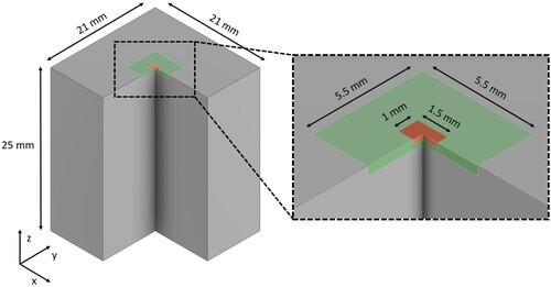
The model geometry is split into three main regions according to the level of detail that is needed for this simulation Figure 3. The first region includes the build plate as well as the surrounding powder bed (Figure 3, grey colour). Since no direct energy input is expected in this region, the conduction of heat only causes relatively low temperature gradients. Therefore a gradually coarsening mesh (min. 200 x 200 x $30\text{μ}{\mathrm{m}}^3$, max. 700 x 700 x $500\text{μ}{\mathrm{m}}^3$) is used in this region. A medium sized mesh (50 x 50 x $10\text{μ}{\mathrm{m}}^3$) is used in the areas where the coarser macroscale energy input model is used (Figure 3, green colour). The mesh size in this region is optimised for an accurate modelling of the energy input and heat conduction, but is not optimised for the analysis of tempering effects. In order to accurately model the mesoscale energy input as well as the phase transformations and localised tempering effects a third region is added for the cube (Figure 3, orange colour). This ROI has the finest mesh (20 x 20 x $3\text{μ}{\mathrm{m}}^3$) in order to to fully use the potential of the mesoscale simulation models. The ROI is located in the centre of the cube for this study, but could be freely moved in order to simulate other regions of interest such as overhanging areas or bottlenecks. Therefore, more complex geometries such as helical springs could be simulated. The only limitation is the resolution of the used element size, since a few elements are needed in order to resolve the geometric features and the resulting temperature profile efficiently. The ROI consisted of 5 lines for the multiscale approach and 9 lines for the quasi-mesoscale approach for this study. The geometry was meshed with first-order hexahedral elements of the Abaqus type DC3D8 and the regions were connected by the *TIE boundary condition in Abaqus.

Figure 3. Schematic cut-view representation of the model geometry, split into three regions: combined volume for build plate and powder bed (outside), printed sample and ROI (center).

A sensitivity analysis (variation of plus and minus one magnitude) regarding the heat losses was conducted as part of this study, with no significant differences noted for the temperature profile during the process. Consequently, the constant heat transfer coefficient h equal to $20\mathrm{W}{\mathrm{m}}^{-2}{\mathrm{K}}^{-1}$ [29] was employed. This coefficient was coupled with the surface temperature T in Kelvin and the ambient air temperature $T_{air}$ which corresponds to room temperature, specifically 293.16 K. The dissipation of heat through convection was delineated utilising the *SFILM keyword within the Abaqus software. Similarly, the heat losses through radiation were modelled with the *SRADIATE keyword in Abaqus Equation (3(3) $q_{rad.}=ϵ\sigma (T^4-T_{air}^4)$(3) ). An emissivity of $ϵ=0.5$ [29], the Stefan-Boltzmann constant σ, the surface temperature T in Kelvin and the air temperature $T_{air}$ were used. (2) $q_{conv.}=h(T-T_{air})$(2) (3) $q_{rad.}=ϵ\sigma (T^4-T_{air}^4)$(3)

2.4.4. Simulation module: phase dependent thermal material model

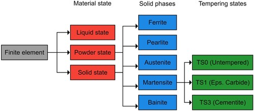
In this section, the material properties and the models used for this FE simulation are presented. A three-level hierarchical structure was used to represent the material states (solid, liquid, powder), the solid phases (ferrite, pearlite, austenite, bainite, martensite, applied to the solid and powder material states) and the tempering states of martensite (untempered martensite TS0, epsilon carbide precipitation TS1 and cementite precipitation TS3). The Lever rule is used to interpolate the material properties in cases where more than one material state, solid state or tempering state is present at a given time. Figure 4 visualises the hierarchical structure.

Figure 4. Hierarchical structure used for the material model. Including the material states, solid state phases and tempering states.

2.4.5. Solid–liquid transformations

In order to simulate the change of the material state during melting and solidification of the powder or solid material, a linear equation was used to interpolate the current phase fraction between the solidus and liquidus temperature. The melting process is reversible for the solid material state, but irreversible for the powder material state, leading to the change from the powder to the liquid to the solid material state while printing. Due to the highly non linear nature, the heat of fusion was neglected for this study. In order to estimate the irreversible loss of energy in the system, a new simplified function was introduced, limiting the maximum temperature to about 3300 K (slightly above the boiling point of pure iron or stainless steel [30,31]). The constant $c=3\times {10}^8\mathrm{k}\mathrm{J}{\mathrm{k}\mathrm{g}}^{-1}{\mathrm{s}}^{-1}{\mathrm{K}}^{-1}$ was optimised to limit the function to the same maximum process temperature during printing for all used parameter combinations Equation (4(4) $\begin{array}{rl}\mathrm{\Delta }{H}_{e,s}(t,T)& =c\mathrm{\Delta }t(T-3200\mathrm{K})\mathrm{w}\mathrm{i}\mathrm{t}\mathrm{h}\\ & T>3200\mathrm{K}\mathrm{a}\mathrm{n}\mathrm{d}\mathrm{\Delta }t\left(\mathrm{i}\mathrm{n}\mathrm{s}\right)\end{array}$(4) ). (4) $\begin{array}{rl}\mathrm{\Delta }{H}_{e,s}(t,T)& =c\mathrm{\Delta }t(T-3200\mathrm{K})\mathrm{w}\mathrm{i}\mathrm{t}\mathrm{h}\\ & T>3200\mathrm{K}\mathrm{a}\mathrm{n}\mathrm{d}\mathrm{\Delta }t\left(\mathrm{i}\mathrm{n}\mathrm{s}\right)\end{array}$(4) This equation is used in order to minimise the effect of the highly non-linear latent heat of evaporation, as well as qualitatively estimating the loss of energy due to splatter formation during the process. This approach was used because spattering is a complex effect that cannot be directly considered in an FEM-based simulation.

2.4.6. Solid-state phase transformations

The main goal of the simulation was to include temperature-dependent phase transformation models that cover relevant phases of AISI 4140. As suggested by Mioković et al. [32,33], the austenite transformation kinetics were described using the Johnson-Mehl-Avrami-Kolmogorov (JMAK) equation (Equation (5(5) $f=1-\exp (-(b\left(T\right)t{)}^n)$(5) )). The temperature dependent factor $b\left(T\right)$ was determined using the parameter $C=2.84\times {10}^{20}{\mathrm{s}}^{-1}$, the activation energy $\mathrm{\Delta }H=6.7\times {10}^{-19}\mathrm{J}$, the growth exponent $n=1.525$ and the Boltzmann constant $k_B$. (5) $f=1-\exp (-(b\left(T\right)t{)}^n)$(5) (6) $b\left(T\right)=C\exp (-\frac{\mathrm{\Delta }H}{k_{B}T})$(6) The martensite transformation kinetics were modelled utilising the Koistinen-Marburger equation [34] Equation (7(7) $f=1-\exp (-{\alpha }_m(T_{KM}-T\left)\right)$(7) ), with the parameter ${\alpha }_m=0.0176{\mathrm{K}}^{-1}$ adapted from van Bohemen and Sietsma [35] based on the specific chemical composition of the material under consideration. The temperature for martensitic transformation $T_{KM}$ was determined to ${363}^{\circ }\mathrm{C}$ through quenching and tempering experiments conducted in a dilatometer. (7) $f=1-\exp (-{\alpha }_m(T_{KM}-T\left)\right)$(7) A model developed by Kaiser et al. [36] was utilised for the short-time tempering kinetics. Their model was used for this study Equation (8(8) $\dot{f}=(1-f{)}^{r}n{t}^{n}b(T{)}^{n-1}$(8) ). Equation (8(8) $\dot{f}=(1-f{)}^{r}n{t}^{n}b(T{)}^{n-1}$(8) ) employed the parameters relevant to tempering states TS1 and TS3, as outlined in Table 2. (8) $\dot{f}=(1-f{)}^{r}n{t}^{n}b(T{)}^{n-1}$(8) Given the rapid quenching inherent in the PBF-LB process, only martensite formed during the cooling. Although the implementation of transformations into ferrite, pearlite, or bainite was included, these phases were not invoked during the simulations.

Table 2. The temperature dependence of the variable ‘I’ is characterised by a polynomial function of the form $I=\sum _{i=0}^2{a}_i{T}^i$, with the coefficients $a_i$ and the temperature T, measured in Kelvin (K) taken from Kaiser et al. [36].

Quantity	Unit	$a_0$	$a_1$	$a_2$
$r_{{\alpha }^{\mathrm{\prime }}\to {\alpha }_{ϵ}^{\mathrm{\prime }}}$	–	1.0	0	0
$r_{{\alpha }_{ϵ}^{\mathrm{\prime }}\to {\alpha }_C^{\mathrm{\prime }}}$	–	1.5	0	0
$\mathrm{\Delta }{H}_{{\alpha }^{\mathrm{\prime }}\to {\alpha }_{ϵ}^{\mathrm{\prime }}}$	J	$1.75\times {10}^{-19}$	0	0
$\mathrm{\Delta }{H}_{{\alpha }_{ϵ}^{\mathrm{\prime }}\to {\alpha }_C^{\mathrm{\prime }}}$	J	$2.74\times {10}^{-19}$	$1.47\times {10}^{-5}$	$1.5\times {10}^{-6}$
$n_{{\alpha }^{\mathrm{\prime }}\to {\alpha }_{ϵ}^{\mathrm{\prime }}}$	–	0.42	0	0
$n_{{\alpha }_{ϵ}^{\mathrm{\prime }}\to {\alpha }_C^{\mathrm{\prime }}}$	–	1.53	$-1.9\times {10}^{-3}$	$1.5\times {10}^{-6}$
$C_{{\alpha }^{\mathrm{\prime }}\to {\alpha }_{ϵ}^{\mathrm{\prime }}}$	${\mathrm{s}}^{-1}$	$8.79\times {10}^{10}$	0	0
$C_{{\alpha }_{ϵ}^{\mathrm{\prime }}\to {\alpha }_C^{\mathrm{\prime }}}$	${\mathrm{s}}^{-1}$	$5.40\times {10}^{12}$	$-6.78\times {10}^9$	$3.56\times {10}^7$

Note: The units of the coefficients are not explicitly written.

2.4.7. Thermal material properties

The thermal properties were modelled with experimental data from literature. The experimental data available for the face centred cubic (fcc) austenite phase and the body centred cubic (bcc) phases, including ferrite, pearlite, bainite, martensite and the tempered phases by Schwenk et al. [37] were combined into a single continuous fit-function for the heat capacity. Equation (9(9) $f\left(T\right)=A_{min}+\frac{(A_{max}-A_{min})}{1+{\left(\frac{T_0}{T}\right)}^{a_p}}$(9) ) was used with the fit parameters shown in Table 3. The thermal conductivity was fitted separately for both fcc and bcc solid states, due to the opposing trend Table 3. (9) $f\left(T\right)=A_{min}+\frac{(A_{max}-A_{min})}{1+{\left(\frac{T_0}{T}\right)}^{a_p}}$(9) The heat capacity for the powder was set to 60% of the solid state, according to the powder packing density [38]. The thermal conductivity for the powder was fitted to Equation (9(9) $f\left(T\right)=A_{min}+\frac{(A_{max}-A_{min})}{1+{\left(\frac{T_0}{T}\right)}^{a_p}}$(9) ) with only 3.5% of the thermal conductivity of the solid state material at room temperature and 100% at temperatures just beneath the solidus temperature. This fit-function was used in order to reduce the strong non-linearities due to the powder-liquid transformation Table 3. A constant heat capacity of $787\mathrm{J}{\mathrm{k}\mathrm{g}}^{-1}{\mathrm{K}}^{-1}$ was used for the liquid state [39]. The experimental data from Wilthan et al. [39] was used for the thermal conductivity of the liquid state Table 3.

Table 3. Thermal input parameters fitted with data from Wilthan et al. [39] and Schwenk et al. [37].

Quantity	Unit	A${}_{min}$	A${}_{max}$	T${}_0$	$a_p$
$c_p^{Solid}$	$\mathrm{J}{\mathrm{k}\mathrm{g}}^{-1}{\mathrm{K}}^{-1}$	378.82	787.00	589.42	3.75
${\lambda }^{Solid,fcc}$	$\mathrm{W}{\mathrm{m}\mathrm{m}}^{-1}{\mathrm{K}}^{-1}$	$1.28\times {10}^{-2}$	$3.33\times {10}^{-2}$	1122.62	3.36
${\lambda }^{Solid,bcc}$	$\mathrm{W}{\mathrm{m}\mathrm{m}}^{-1}{\mathrm{K}}^{-1}$	$1.77\times {10}^{-2}$	$4.16\times {10}^{-2}$	964.47	−4.80
${\lambda }^{Powder}$	$\mathrm{W}{\mathrm{m}\mathrm{m}}^{-1}{\mathrm{K}}^{-1}$	$4.52\times {10}^{-4}$	$4.64\times {10}^{-2}$	1509.66	5.90
${\lambda }^{Liquid}$	$\mathrm{W}{\mathrm{m}\mathrm{m}}^{-1}{\mathrm{K}}^{-1}$	$2.43\times {10}^{-2}$	$5.50\times {10}^{-2}$	2400.00	4.07

Note: The units of the coefficients are not explicitly written.

2.4.8. Hardness calculation

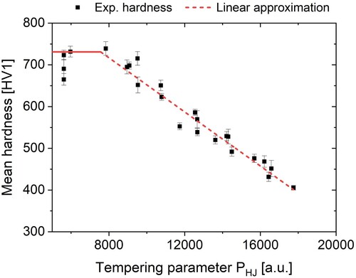
The correlation between hardness and tempering state is measured using the Hollomon-Jaffe parameter, referred to as $P_{HJ}$. This parameter shows a linear relationship with the observed hardness of AISI 4140, even under conditions of high heating rates, as demonstrated by Kaiser et al. [36]. This parameter is extensively applicable to processes characterised by rapid heating and cooling, including induction hardening [8,9,36], laser surface hardening [7] and PBF-LB [3]. To specifically calibrate this parameter for the precise chemical composition of the alloy investigated in this study, samples produced through the as-built process underwent quenching and tempering within a dilatometer. After the quenching phase, the samples were tempered at various constant heating rates between $1^{\circ }\mathrm{C}{\mathrm{s}}^{-1}$ to ${1000}^{\circ }\mathrm{C}{\mathrm{s}}^{-1}$, culminating at final tempering temperatures of ${200}^{\circ }\mathrm{C}$ to ${600}^{\circ }\mathrm{C}$. The obtained temperature profiles were used to compute the $P_{HJ}$ parameter, according to Equation (10(10) $P_{HJ,i}=P_{HJ,i-1}+\frac{T_i}{2.303\cdot {10}^{\frac{P_{HJ,i-1}}{T_i-C}}}\cdot \mathrm{\Delta }t$(10) ). In this equation, $P_{HJ,0}$ is equal to $C{T}_0$, with $T_0$ representing 293.16 K. The constant C depends on the carbon content and was calculated to C = 19.04 [40]. Using Equation (11(11) $\begin{array}{rl}H\left(P_{HJ,i}\right)& =\{\begin{array}{cc}976.1\mathrm{H}\mathrm{V}1-0.0324\mathrm{H}\mathrm{V}1\cdot P_{HJ,i}& P_{HJ,i}>7600\\ 731.0\mathrm{H}\mathrm{V}1& P_{HJ,i}\le 7600\end{array}\end{array}$(11) ), the hardness values resulting from these tempering experiments are calculated and represented graphically against the $P_{HJ}$ parameter in Figure 5. (10) $P_{HJ,i}=P_{HJ,i-1}+\frac{T_i}{2.303\cdot {10}^{\frac{P_{HJ,i-1}}{T_i-C}}}\cdot \mathrm{\Delta }t$(10) (11) $\begin{array}{rl}H\left(P_{HJ,i}\right)& =\{\begin{array}{cc}976.1\mathrm{H}\mathrm{V}1-0.0324\mathrm{H}\mathrm{V}1\cdot P_{HJ,i}& P_{HJ,i}>7600\\ 731.0\mathrm{H}\mathrm{V}1& P_{HJ,i}\le 7600\end{array}\end{array}$(11)

Figure 5. Hardness values of quenched and tempered samples with different heating rates and maximum tempering temperatures plotted over the calculated tempering parameter for each experiment. The linear approximation used for this study is visualised with a dashed line.

To assess the bulk hardness in the simulated components, the ROI was examined. This examination extended to at least four layers beneath the surface. For the highest VED scenarios, the analysis was extended to up to six layers to ensure that equilibrium hardness levels were achieved for each simulated VED configuration. Afterwards, the mean hardness, along with its standard deviation, was computed based on the hardness values attributed to individual finite elements present within this designated area.

The proposed FE simulation approach for the PBF-LB process was adeptly harnessed by incorporating temperature and phase-dependent tempering effects into the simulation model. This strategic approach facilitated a thorough exploration of the hardness profile throughout the process and allowed for a detailed investigation of various parameter combinations.

2.4.9. Optics modelling

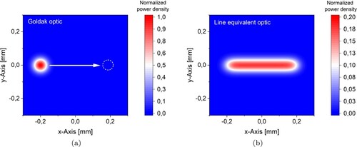
In order to combine the two scales (macro- and mesoscale) into one simulation model, two different optic models were used for the energy input, both visualised in Figure 6 (the differences in normalised power density should be noted).

Figure 6. Visualisation of the two optic models used for this study. With the Goldak type optic (a) and the line equivalent optic (b).

2.4.10. Goldak type optic

The Goldak type optic uses a double-ellipsoid as the heat source which was originally created for welding process simulations [41], but was adapted for the laser based additive manufacturing process like PBF-LB [23,42,43]. This optic is then moved across the part according to the trajectory created by the G-Code. It shows a high accuracy in the high and low temperature regions [23]. The volume heat flux is calculated in the Abaqus subroutine DFLUX according to the modified Goldak equation [23,42], shown in Equation (12(12) $\omega (x,y,z,t)=\frac{2\eta P}{abc\pi \sqrt{\pi }}\cdot \exp (-\frac{{(x-v_{x}t)}^2}{a^2}-\frac{{(y-v_{y}t)}^2}{b^2}-\frac{z^2}{c^2})$(12) ). (12) $\omega (x,y,z,t)=\frac{2\eta P}{abc\pi \sqrt{\pi }}\cdot \exp (-\frac{{(x-v_{x}t)}^2}{a^2}-\frac{{(y-v_{y}t)}^2}{b^2}-\frac{z^2}{c^2})$(12) The laser power P is directly taken from the experiment, with the parameters a and b equal to the laser spot diameter [23]. Since the parameter c, and the laser absorption coefficient η are dependent on the laser power P, the laser speed in x-direction $v_x$ and the laser speed in y-direction $v_y$, they were fitted to the experimental results Section 3.1.

2.4.11. Line equivalent optic

The line equivalent optic is based on the Goldak optic, but is simplified in order to optimise the computation cost for macroscale simulations. This type of optic averages the energy input over a longer time period (a complete scan path in this case), while maintaining the same energy input for each finite element compared to the Goldak model. A Python script is used to calculate the equivalent optic for each line with the actual line length, laser speed and laser power by moving the Goldak model over a 3D mesh. The volume heat flux is integrated for each finite element and is then divided by the total time to process this scan path in order to get the average volume heat flux. The results are then fitted with three dimensional rectangular Gaussian function in order to be used in the Abaqus DFLUX subroutine Equation (13(13) $f(x,y,z)=a\cdot \exp (-{\left(\frac{x^2}{2{\sigma }_x^2}\right)}^{P_x}-{\left(\frac{y^2}{2{\sigma }_y^2}\right)}^{P_y}-{\left(\frac{z^2}{2{\sigma }_z^2}\right)}^{P_z})$(13) ). (13) $f(x,y,z)=a\cdot \exp (-{\left(\frac{x^2}{2{\sigma }_x^2}\right)}^{P_x}-{\left(\frac{y^2}{2{\sigma }_y^2}\right)}^{P_y}-{\left(\frac{z^2}{2{\sigma }_z^2}\right)}^{P_z})$(13) Similar approaches for equivalent optics were already successfully used for the laser surface hardening process [7,44]. This simplification reduces the computational cost by allowing the usage of larger time and spacial increments during the simulation, while reducing the accuracy in near field temperature prediction. Due to the exact same energy input as the Goldak model, the far field temperature can be calculated with high accuracy.

3. Results and discussion

3.1. Dimensions of the hardened zone of single beads

In order to validate the proposed simulation models for the PBF-LB process, the single beads printed on top of the samples without additional powder were used. Due to the microstructure of the single beads and the surrounding area, a direct measurement of the melt pool sizes is unreliable. Since both the hardened zone (HZ) and the previously melted zone show a martensitic microstructure after cooling to room temperature, the boundary between both is not easily visible. Therefore, the size of the hardened zone is used for the comparison of the simulation and the experiment, due to the visual difference between the newly hardened zone and the surrounding highly tempered martensitic microstructure Figure 7. The width and depth of the HZ were experimentally measured on the cut surface of the samples. All samples used for the validation were excluded from the parametrisation data set and were only used for the purpose of this validation. The simulations used the same process parameters as their experimental counterparts and the Goldak type energy input as proposed in Section 2.4.9. Both the absorption coefficient η and the c parameter of the Goldak function were fitted to a logistic function Equation (14(14) $f(P,v)=A_{min}+\frac{A_{max}-A_{min}}{1+{\left(\frac{x_0\cdot v}{P}\right)}^{a_p}}$(14) ). (14) $f(P,v)=A_{min}+\frac{A_{max}-A_{min}}{1+{\left(\frac{x_0\cdot v}{P}\right)}^{a_p}}$(14) For the absorption coefficient, the limits $A_{min}$ and $A_{max}$ were set to 0.3 and 0.9, respectively [45–47]. The function was then fitted to the experimental data with $x_0=0.214\mathrm{J}{\mathrm{m}\mathrm{m}}^{-1}$ and $a_p=6.9$. Likewise, for the Goldak parameter c the limits $A_{min}$ and $A_{max}$ were set to the layer height as the minimal absorption depth and three times the layer height as the maximum absorption depth in the stable process window, respectively. The function was then fitted to the experimental data with $x_0=0.282\mathrm{J}{\mathrm{m}\mathrm{m}}^{-1}$ and $a_p=9$. 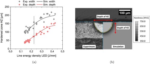The proposed FEM simulation generally predicts the width and depth of the HZ with only small deviations for the heat conduction welding regime Figure 8. Due to bigger scattering of the experimentally measured sizes of the HZ near the keyhole welding regime (melt pool instability), the quality of the fit also decreases while still predicting an accurate mean size of the width and depth of the HZ.

Figure 7. Light microscopic image of a exemplary etched cross section of a single bead printed on top of the sample without additional powder. The effective top surface, the boundary of the hardened zone and the width and depth measurements are highlighted in this image.

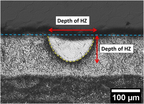
Figure 8. Visualisation of the (a) measured experimental width and depth of HZ of the single beads on top of the printed parts and prediction of width and depth of the HZ of the proposed FEM simulation and (b) direct comparison of experiment and simulation for a LED of $0.225\mathrm{J}{\mathrm{m}\mathrm{m}}^{-1}$.

3.2. Global thermal history of printed cubes

The temperature profile of the multiscale approach were compared to the macroscale and quasi-mesoscale approach for a VED of $65\mathrm{W}{\mathrm{m}\mathrm{m}}^{-3}$ Figure 9 (a) and a VED of $115\mathrm{W}{\mathrm{m}\mathrm{m}}^{-3}$ Figure 9(b) in order to validate the temperature profile. With the workstation used for this study (See Section 2.3), simulation times of about 7 h per layer for the macroscale, 16 h per layer for the multiscale and 32 h per layer for the quasi-mesoscale simulation were achieved Table 4.

Figure 9. Predicted temperature profile of all three simulation models for a VED of $65\mathrm{J}{\mathrm{m}\mathrm{m}}^{-3}$ (a) and a VED of $115\mathrm{J}{\mathrm{m}\mathrm{m}}^{-3}$ (b).

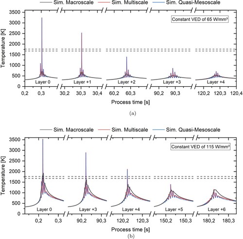
Table 4. Simulation runtime and relative runtime compared to the quasi-mesoscale for all three used simulation approaches.

Simulation approach	Runtime [h]	Relative runtime [%]
Macroscale	7	22
Multiscale	16	50
Quasi-Mesoscale	32	100

The temperature profile starts at layer zero, where the finite element is added to the simulation as part of the new powder layer. The temperature rises slowly at the start of the laser process of every layer, as the perimeter and hatch lines further away from the finite element are printed (far-field energy input). There is no significant difference noted for all three models during this time period. As the laser gets closer to the finite element, the temperature rises significantly faster. The maximum temperature of every layer is reached when the laser directly moves over the finite element, resulting in the shortest distance to the energy input. Depending on the used model, VED and analysed layer the maximum temperature of every layer varies significantly. Notably, an increase in the number of layers above the finite element leads to a reduction in the maximum temperature. While the multiscale and quasi-mesoscale models reach the same maximum temperature for all additional layers and both VEDs, the full macroscale simulation significantly underestimates the maximum temperature in this near-field region. Since this error wasn't noted for the multiscale simulation, a two scan line wide distance from the macroscale zone to the temperature measurement point was sufficient to neglect errors in heat dissipation of the macroscale models. Due to the conduction to the baseplate and already printed regions, the part cools down rapidly, even if the laser still melts the powder further away from the finite element. During this cooling process the temperature profile of all three models are approaching the same equilibrium temperature. Besides the differences of the temperature profile regarding the simulation models with a constant VED, a significant difference in the resulting temperature profile is noted for the variation of the VED itself. A lower VED, and therefore lower energy input, reduces the maximum temperatures, the size of the heat affected zone (HAZ) and significantly increases the heating and cooling rates during the process Figure 9(a). The tempering effects occurring during the process can be categorised into an in-layer tempering effect caused by the printing of adjacent lines and a layer-wise tempering effect caused by the additional layers printed on top. In case of the lowest analysed VED, the temperature falls below the austenitisation temperature during the hatching process, allowing for an in-layer hardening, tempering and re-austenitisation process when the adjacent line is printed. This effect is not noted for the highest analysed VED in this study. Since the cooling rates are lower due to the higher energy input, a more uniform heat distribution is formed. This leads to an austenitic region that spans multiple printed lines, with a martensitic transformation outside the tempering zone of the laser, preventing the in-layer tempering effects. In both cases the main tempering effect is caused by the addition of the next layers printed on top, leading to a cyclic re-austenitisation, melting, hardening and tempering process.

The large difference in the near-field temperature curve can be explained by the coarser approximation of the energy distribution of the line-equivalent optic type compared to the Goldak optic type used in the ROI of the multi- and quasi-mesoscale optic. The further away the energy input is located from the finite element under investigation, the smaller the error of this coarser approximation gets. This temperature difference is also more noticeable for lower VEDs compared to the higher VEDs, due to the lower equilibrium temperature and higher heating and cooling rates. Since both optic models use the same energy input, the temperature profile converges in the far-field, because small differences in the timing and distribution of the energy density over time are smoothed by the thermal conductivity of the printed part.

3.3. Bulk hardness of printed cubes

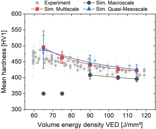
The calculated temperature profiles of the three simulation models enable the calculation of multiple material properties. This section focuses on the resulting bulk hardness calculated by the incremental Hollomon-Jaffe approach compared to the experimental bulk hardness measurements. The minimum and maximum VED were selected according to the results of the experimental parameter study, in order to only simulate VEDs of the stable process window. Figure 10 shows the resulting hardness of the three simulation models compared to the experimental measurements of the conducted parameter study. While the predicted hardness of the multi- and quasi-mesoscale simulations are within the scatter band of the experimental results, the results of the macroscale simulation are lower than the experimental measurements. No austenitisation and therefore no tempering effect was noted for the macroscale simulations of a VED lower than $90\mathrm{J}{\mathrm{m}\mathrm{m}}^{-3}$, showing the unchanged initialisation hardness of the powder layer, which was set to 350 HV1. Only small differences within the standard deviation of both simulations are noted while comparing the multiscale and quasi-mesoscale simulations.

Figure 10. Predicted mean bulk hardness for different VEDs by the three simulation models compared to experimental data.

Due to the tempering mechanisms of the Q&T steels, the resulting hardness after cooling is strongly dependent on the local thermal history. Furthermore, the most important time interval of the simulation is the time between the final austenitisation of the finite element and the subsequent layers, since it is characterising the tempering process. The resulting hardness of a finite element after each printed layer with a VED of $115\mathrm{J}{\mathrm{m}\mathrm{m}}^{-3}$ is visualised in Figure 11, with the significant time interval for the hardness prediction highlighted in light green. The martensitic hardening and tempering in the layers before the final austenitisation is nullified by the following high temperature peaks reaching above the austenitisation or even the melting temperature of the finite element. For all additional layers simulated after the crucial time interval (highlighted in light green in Figure 11), the maximum temperature reached is not enough to further temper the finite element. Since the tempering process is strongly dependent on time and temperature, the low accumulated time at temperatures lower than the maximum tempering temperature is not sufficient to further reduce the predicted bulk hardness. The equilibrium bulk hardness is reached two layers after the final austenitisation. The difference in the resulting bulk hardness can be explained by the temporal shift of the final austenitisation between the macroscale and the multi- and quasi-mesoscale models. The final austenitisation occurs one layer earlier in the macroscale simulation, leading to slightly higher temperatures during the tempering interval, therefore reducing the bulk hardness compared the multi- and quasi-mesoscale simulation models. Another factor reducing the bulk hardness of the macroscale simulation is the difference in temperature during the near-field cooling phase (See Figure 9(b) in layer +6), effectively increasing the tempering effect due to a longer time interval at higher temperatures. The small deviations of the temperature profile during the near-field cooling of the multi- and quasi-mesoscale simulations result in negligible differences of the bulk hardness, effectively validating the multiscale approach with its significantly smaller ROI size.

3.4. Local microstructure of printed cubes

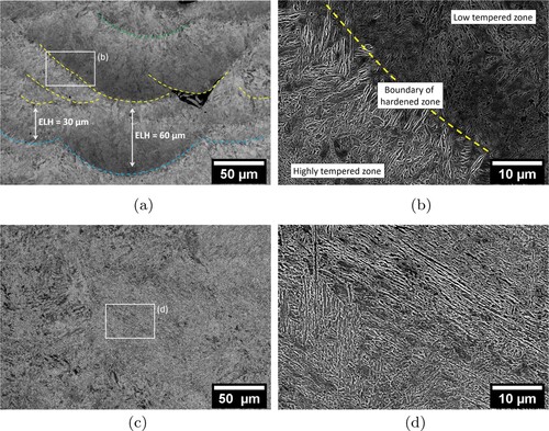
In this section the effect of different VEDs on local microstructure and hardness gradients is evaluated. Two samples of the experimental parameter study with a VED of $65\mathrm{J}{\mathrm{m}\mathrm{m}}^{-3}$ (minimum) and a VED of $115\mathrm{J}{\mathrm{m}\mathrm{m}}^{-3}$ (maximum) were analysed. The SEM recordings of the cut sections reveal the differences in microstructure for both VEDs (See Figure 12). The sample with the lowest VED of $65\mathrm{J}{\mathrm{m}\mathrm{m}}^{-3}$ shows a more pronounced graded microstructure with previous boundaries of the hardened zone still visible Figure 12(a–b). The former boundaries of the HZ are highlighted with a yellow line. Two distinct regions are recognised in this sample. The region with a high tempering state just beneath a former boundary of the hardened zone is characterised by a network of cementite precipitations at lath boundaries Figure 12(b). The region on top of the former boundary of the hardened zone is characterised by a lower tempering state just inside a former melt pool boundary with less cementite precipitations. Furthermore, the perceived effective layer height (ELH), measured from one boundary of the hardened zone to the next, varies from $30\text{μ}\mathrm{m}$ to $60\text{μ}\mathrm{m}$ in this sample Figure 12(a). This variation of effective layer height is likely caused by melt pool instability, as well as defects on the surface such as splatter, humping or balling, due to the low VED used for this sample. In contrary, the sample with the highest VED of $115\mathrm{J}{\mathrm{m}\mathrm{m}}^{-3}$ shows a rather uniform microstructure of tempered martensite and precipitated cementite. Previous boundaries of the hardened zone are barely visible in the SEM images Figure 12(c–d). No significant localised differences of the microstructure are visible for the sample with a VED of $115\mathrm{J}{\mathrm{m}\mathrm{m}}^{-3}$. The microstructure appears to be more homogeneous, showing coarser cementite precipitate. Due to the orientation of the martensite laths visible in Figure 12(d), prior austenite grains and therefore former melt pool boundaries could be reconstructed in future work. Since it was out of scope for this work to compare the quantitative difference in cementite shapes and sizes in detail, just the qualitative differences in estimated tempering states between the two VEDs were used to compare to the microstructure prediction of the proposed multiscale FEM simulation.

Figure 11. Predicted hardness of a finite element after each layer is printed with a constant VED of 115 Jmm–3. The marked region highlights the crucial time interval for the hardness prediction.

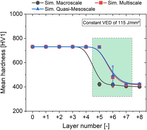
Figure 12. SEM images of the microstructure of the sample with a VED of $65\mathrm{J}{\mathrm{m}\mathrm{m}}^{-3}$ (a–b) and a VED of $115\mathrm{J}{\mathrm{m}\mathrm{m}}^{-3}$ (c–d).

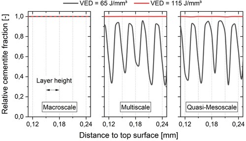
In order to validate the simulation models for the qualitative microstructure prediction, simulations with the same parameter combinations were conducted. As a result of the approximations taken for the simulation models, it is not possible to simulate separate carbides in the matrix, but to show localised differences in the tempering. Therefore, the model by Kaiser et al. [36] estimates the current tempering state by calculating the relative cementite fraction (current cementite fraction divided by max. possible cementite fraction) for each integration point of the FEM simulation. Figure 13 visualises the simulated depth profile of relative cementite fraction after the printing process for all three simulation models and therefore the local microstructure gradients. An almost fully tempered, homogeneous microstructure throughout the sample is predicted for the high VED of $115\mathrm{J}{\mathrm{m}\mathrm{m}}^{-3}$, with no difference between all three simulation models (Figure 13, red line). These predicted results are qualitatively comparable with the lack of microstructure gradients observed by the experiment for the same VED Figure 12(c). A difference for the predicted microstructure is noted for the lower VED of $65\mathrm{J}{\mathrm{m}\mathrm{m}}^{-3}$ (Figure 13, blue line). While a graded microstructure is predicted by the multiscale and quasi-mesoscale simulation models (Figure 13, blue line, center and right), a homogeneous tempering state is predicted by the fully macroscale model (Figure 13, blue line, left). Figure 13 additionally reveals a cyclic pattern of lower and higher tempered areas for the lower VED sample, also observed in the experiment. The maxima and minima of the relative cementite fraction are approximately $30\text{μ}\mathrm{m}$ apart, which is consistent with the nominal powder layer height. Given the idealised layer height and melt pool geometry for the simulation, a direct comparison of the cyclic pattern with experimental results is not possible.

The identified differences in local microstructure are caused by the temperature gradient, and therefore directly influencing the size of the HAZ. Since the highest tempering temperatures are reached here, this zone is the most important area for tempering (See Section 3.3). The thermal gradients in this zone will be decisive for the resulting microstructure. The higher VED leads to lower thermal gradients inside the $30\text{μ}\mathrm{m}$ zone, which directly corresponds to the more homogeneous microstructure in the experiment, as well as the FEM simulation. Due to the higher thermal gradients inside the $30\text{μ}\mathrm{m}$ zone, a graded microstructure is predicted by the simulation and shown in the experiment for the lower VED sample. The considerable difference of thermal gradients is shown in Figure 9. While the temperature of samples manufactured with a VED of $65\mathrm{J}{\mathrm{m}\mathrm{m}}^{-3}$ almost instantly falls below ${200}^{\circ }\mathrm{C}$ due to conduction, the samples manufactured with the higher VED are cooling down more slowly. Overall, these results indicate that the multiscale and quasi-mesoscale simulations are able to qualitatively predict the tempering states caused by different process parameter combinations.

Figure 13. Calculated relative cementite fraction by all three simulation models for the minimum and maximum VED in the printed part. Visualizing local microstructure gradients predicted by the simulation.

4. Conclusion

A new multiscale simulation model for the PBF-LB process of martensitic steels was introduced. Combining macro- and mesoscale models into one simulation reduced the computational cost, while retaining a high accuracy. This new approach therefore offers several advantages over other simulation methods, as well as the experimental trial-and-error method, in order to further optimise the process parameter selection for functionally graded parts through intrinsic heat treatment. Therefore, the simulation model offers a systematic approach to process optimisation. By comparing and linking the results of the parameter study, the following conclusions can be drawn:

• An FEM simulation model for conventional heat treatment processes (laser surface hardening, induction hardening) was successfully adapted and extended for the process simulation of the PBF-LB process. A multiscale FEM simulation model was introduced to combine methods from the macroscale and mesoscale into one simulation model in order to maintain the accuracy of the mesoscale and significantly reduce the computational cost (which enables the simulation on the full part scale). The Goldak and line equivalent optic models of the two scales were adapted for the experimental results of printed single beads.

• A hardness prediction model based on the Hollomon-Jaffe parameter was introduced for the PBF-LB process, considering the actual chemical composition of the printed parts. The predicted bulk hardness of the simulations was compared to the experimental measurements in order to validate the simulation models. While the multiscale and quasi-mesoscale simulation models were able to predict the hardness values for all analysed volume energy densities (VED), the macroscale was not able to accurately predict the hardness for all VEDs. The macroscale simulations slightly underestimate the hardness for the higher VEDs, but is not able to predict the hardness of sample processed with a VED lower than $90\mathrm{J}{\mathrm{m}\mathrm{m}}^{-3}$ due to the approximation of the energy input model.

• Additional microstructure analysis was conducted to compare the simulation with the experiment. While the multiscale and quasi-mesoscale simulation models were able to predict the graded microstructure for higher VED samples, the macroscale was not able to accurately predict the localised tempering state.

• Since both the localised microstructure and the bulk hardness are directly related to the calculated temperature profile, the thermal simulation could be validated for the whole stable process parameter range of the AISI 4140 Q&T steel.

The findings of this study can be further used to improve the parameter combinations during the PBF-LB process, especially for manufacturing functionally graded parts with a localised adaption of process parameter sets, as well as for more detailed simulations.

Acknowledgments

The authors thank Gregor Graf and Philipp Schwarz from Rosswag Engineering GmbH for manufacturing the samples used in this study. This research did not receive any specific grant from funding agencies in the public, commercial, or not-for-profit sectors. We acknowledge support by the KIT-Publication Fund of the Karlsruhe Institute of Technology.

Disclosure statement

No potential conflict of interest was reported by the author(s).

References

- Hearn W, Hryha E. Effect of carbon content on the processability of Fe-C alloys produced by laser based powder bed fusion. Front Mater. 2022;8:547. doi: 10.3389/fmats.2021.800021
- Bobel A, Hector LG, Chelladurai I, et al. In situ synchrotron X-ray imaging of 4140 steel laser powder bed fusion. Materialia. 2019;6:Article ID 100306. doi: 10.1016/j.mtla.2019.100306
- Damon J, Koch R, Kaiser D, et al. Process development and impact of intrinsic heat treatment on the mechanical performance of selective laser melted AISI 4140. Addit Manuf. 2019;28:275–284. doi: 10.1016/j.addma.2019.05.012
- Hearn W, Steinlechner R, Hryha E. Laser-based powder bed fusion of non-weldable low-alloy steels. Powder Metall. 2022;65(2):121–132. doi: 10.1080/00325899.2021.1959695
- Hearn W, Harlin P, Hryha E. Development of powder bed fusion – laser beam process for AISI 4140, 4340 and 8620 low-alloy steel. Powder Metall. 2023;66(2):94–106. doi: 10.1080/00325899.2022.2134083
- Shi C, Dietrich S, Schulze V. Parameter optimization and mechanical properties of 42CrMo4 manufactured by laser powder bed fusion. Int J Adv Manuf Technol. 2022;121(3-4):1899–1913. doi: 10.1007/s00170-022-09474-9
- Schüßler P, Damon J, Mühl F, et al. Laser surface hardening: a simulative study of tempering mechanisms on hardness and residual stress. Comput Mater Sci. 2023;221:Article ID 112079. doi: 10.1016/j.commatsci.2023.112079
- Kaiser D, Damon J, Mühl F, et al. Experimental investigation and finite-element modeling of the short-time induction quench-and-temper process of AISI 4140. J Mater Process Technol. 2020;279:Article ID 116485. doi: 10.1016/j.jmatprotec.2019.116485
- Mühl F, Damon J, Dietrich S, et al. Simulation of induction hardening: simulative sensitivity analysis with respect to material parameters and the surface layer state. Comput Mater Sci. 2020;184:Article ID 109916. doi: 10.1016/j.commatsci.2020.109916
- Rudnev V, Loveless D, Cook RL, et al. Handbook of induction heating. 1st ed. Boca Raton (FL): CRC Press; 2002. (Manufacturing engineering and materials processing).
- Krakhmalev P, Yadroitsava I, Fredriksson G, et al. In situ heat treatment in selective laser melted martensitic AISI 420 stainless steels. Mater Des. 2015;87:380–385. doi: 10.1016/j.matdes.2015.08.045. https://www.sciencedirect.com/science/article/pii/S026412751530294X
- Jägle EA, Sheng Z, Kürnsteiner P, et al. Comparison of maraging steel micro- and nanostructure produced conventionally and by laser additive manufacturing. Materials (Basel, Switzerland). 2017;10(1):8. doi: 10.3390/ma10010008
- Kürnsteiner P, Wilms MB, Weisheit A, et al. Massive nanoprecipitation in an Fe-19Ni-xAl maraging steel triggered by the intrinsic heat treatment during laser metal deposition. Acta Mater. 2017;129:52–60. doi: 10.1016/j.actamat.2017.02.069. https://www.sciencedirect.com/science/article/pii/S1359645417301702
- Kürnsteiner P, Benjamin Wilms M, Weisheit A, et al. High-strength Damascus steel by additive manufacturing. Nature. 2020;582(7813):515–519. doi: 10.1038/s41586-020-2409-3
- Hearn W, Lindgren K, Persson J, et al. In situ tempering of martensite during laser powder bed fusion of Fe-0.45C steel. Materialia. 2022;23:Article ID 101459. doi: 10.1016/j.mtla.2022.101459
- Zaeh MF, Branner G. Investigations on residual stresses and deformations in selective laser melting. Prod Eng. 2010;4(1):35–45. doi: 10.1007/s11740-009-0192-y
- Prabhakar P, Sames WJ, Dehoff R, et al. Computational modeling of residual stress formation during the electron beam melting process for Inconel 718. Addit Manuf. 2015;7:83–91. doi: 10.1016/j.addma.2015.03.003. https://www.sciencedirect.com/science/article/pii/S2214860415000160
- Williams RJ, Davies CM, Hooper PA. A pragmatic part scale model for residual stress and distortion prediction in powder bed fusion. Addit Manuf. 2018;22:416–425. doi: 10.1016/j.addma.2018.05.038. https://www.sciencedirect.com/science/article/pii/S2214860418300514
- Denlinger ER, Irwin J, Michaleris P. Thermomechanical modeling of additive manufacturing large parts. J Manuf Sci Eng. 2014;136(6):Article ID 061007. doi: 10.1115/1.4028669
- Du Y, You X, Qiao F, et al. A model for predicting the temperature field during selective laser melting. Results Phys. 2019;12:52–60. doi: 10.1016/j.rinp.2018.11.031
- Marques BM, Andrade CM, Neto DM, et al. Numerical analysis of residual stresses in parts produced by selective laser melting process. Procedia Manuf. 2020;47:1170–1177. doi: 10.1016/j.promfg.2020.04.167
- Noll I, Bartel T, Menzel A. A computational phase transformation model for selective laser melting processes. Comput Mech. 2020;66(6):1321–1342. doi: 10.1007/s00466-020-01903-4
- Hocine S, van Swygenhoven H, van Petegem S. Verification of selective laser melting heat source models with operando X-ray diffraction data. Addit Manuf. 2021;37:Article ID 101747. doi: 10.1016/j.addma.2020.101747
- Cook PS, Murphy AB. Simulation of melt pool behaviour during additive manufacturing: underlying physics and progress. Addit Manuf. 2020;31:Article ID 100909. doi: 10.1016/j.addma.2019.100909
- Ransenigo C, Tocci M, Palo F, et al. Evolution of melt pool and porosity during laser powder bed fusion of Ti6Al4V alloy: numerical modelling and experimental validation. Lasers Manuf Mater Process. 2022;9(4):481–502. doi: 10.1007/s40516-022-00185-3
- Gh Ghanbari P, Mazza E, Hosseini E. Adaptive local-global multiscale approach for thermal simulation of the selective laser melting process. Addit Manuf. 2020;36:Article ID 101518. doi: 10.1016/j.addma.2020.101518
- Bresson Y, Tongne Aèvi, Baili M, et al. Global-to-local simulation of the thermal history in the laser powder bed fusion process based on a multiscale finite element approach. Int J Adv Manuf Technol. 2023;127(9-10):4727–4744. doi: 10.1007/s00170-023-11427-9
- Schindelin J, Arganda-Carreras I, Frise E, et al. Fiji: an open-source platform for biological-image analysis. Nat Methods. 2012;9(7):676–682. doi: 10.1038/nmeth.2019
- Peyre P, Aubry P, Fabbro R, et al. Analytical and numerical modelling of the direct metal deposition laser process. J Phys D: Appl Phys. 2008;41(2):Article ID 025403. doi: 10.1088/0022-3727/41/2/025403
- Mundra K, DebRoy T. Toward understanding alloying element vaporization during laser beam welding of stainless steel: a comprehensive model is proposed to predict vaporization rates during welding. Predictions are compared with experimental data. Welding research supplement; 1993.
- Savvatimskiy AI, Onufriev SV. Specific heat of liquid iron from the melting point to the boiling point. High Temp. 2018;56(6):933–935. doi: 10.1134/S0018151X18060202
- Mioković T, Schwarzer J, Schulze V, et al. Description of short time phase transformations during the heating of steels based on high-rate experimental data. J Phys IV. 2004;120:591–598. doi: 10.1051/jp4:2004120068
- Mioković T, Schulze V, Vöhringer O, et al. Prediction of phase transformations during laser surface hardening of AISI 4140 including the effects of inhomogeneous austenite formation. Mater Sci Eng A. 2006;435-436:547–555. doi: 10.1016/j.msea.2006.07.037
- Koistinen DP, Marburger RE. A general equation prescribing the extent of the austenite-martensite transformation in pure iron-carbon alloys and plain carbon steels. Acta Materialia. 1959;7(1):59–60. doi: 10.1016/0001-6160(59)90170-1
- van Bohemen SMC, Sietsma J. Martensite formation in partially and fully austenitic plain carbon steels. Metall Mater Trans A. 2009;40(5):1059–1068. doi: 10.1007/s11661-009-9796-2
- Kaiser D, de Graaff B, Dietrich S, et al. Investigation of the precipitation kinetics and microstructure evolution of martensitic AISI 4140 steel during tempering with high heating rates. Metall Res Technol. 2018;115(4):404. doi: 10.1051/metal/2018026
- Schwenk M, Hoffmeister Jürgen, Schulze V. Experimental determination of process parameters and material data for numerical modeling of induction hardening. J Mater Eng Perform. 2013;22(7):1861–1870. doi: 10.1007/s11665-013-0566-3
- Wischeropp TM, Emmelmann C, Brandt M, et al. Measurement of actual powder layer height and packing density in a single layer in selective laser melting. Addit Manuf. 2019;28:176–183. doi: 10.1016/j.addma.2019.04.019
- Wilthan B, Reschab H, Tanzer R, et al. Thermophysical properties of a Chromium–Nickel–Molybdenum steel in the solid and liquid phases. Int J Thermophys. 2008;29(1):434–444. doi: 10.1007/s10765-007-0300-1
- Hollomon JH, Jaffe LD. Time-temperature relations in tempering steel. Trans AIME. 1945;162:223–249.
- Goldak J, Chakravarti A, Bibby M. A new finite element model for welding heat sources. Metall Trans B. 1984;15(2):299–305. doi: 10.1007/BF02667333
- Zhang Q, Xie J, Gao Z, et al. A metallurgical phase transformation framework applied to SLM additive manufacturing processes. Mater Des. 2019;166:Article ID 107618. doi: 10.1016/j.matdes.2019.107618
- Zhang Z, Huang Y, Rani Kasinathan A, et al. 3-Dimensional heat transfer modeling for laser powder-bed fusion additive manufacturing with volumetric heat sources based on varied thermal conductivity and absorptivity. Opt Laser Technol. 2019;109:297–312. doi: 10.1016/j.optlastec.2018.08.012
- Cordovilla F, García-Beltrán A, Montealegre MA, et al. Development of model-based laser irradiation customization strategies for optimized material phase transformations in the laser hardening of Cr-Mo steels. Mater Des. 2021;199:Article ID 109411. doi: 10.1016/j.matdes.2020.109411
- Rubenchik A, Wu S, Mitchell S, et al. Direct measurements of temperature-dependent laser absorptivity of metal powders. Appl Opt. 2015;54(24):7230–7233. doi: 10.1364/AO.54.007230
- Boley CD, Mitchell SC, Rubenchik AM, et al. Metal powder absorptivity: modeling and experiment. Appl Opt. 2016;55(23):6496–6500. doi: 10.1364/AO.55.006496
- Trapp J, Rubenchik AM, Guss G, et al. In situ absorptivity measurements of metallic powders during laser powder-bed fusion additive manufacturing. Appl Mater Today. 2017;9:341–349. doi: 10.1016/j.apmt.2017.08.006