Detection and quantitative evaluation of surface defects in wire and arc additive manufacturing based on 3D point cloud

ABSTRACT

Wire and Arc Additive Manufacturing (WAAM) with high efficiency and low-cost is an economical choice for the rapid fabrication of medium-to-large-sized metallic components and has attracted great attention from scholars and entrepreneurs in recent years. However, defects such as porosity, and humps, could occur occasionally after each layer of deposition on weld bead surfaces due to disturbances and process abnormities. Detection and quantitative evaluation of weld bead defects is crucial to ensure successful deposition and the quality of the entire component. In this paper, a novel defect detection and evaluation system was developed for WAAM utilizing machine vision technology. The system incorporated new defect detection algorithms based on analysing the 2D curvature of the weld bead height curve and the 3D curvature of the weld bead point cloud. Furthermore, a defect evaluation algorithm was developed based on reconstructing the normal weld bead contour using geometric features extracted from the accumulated point cloud. This system enables the automatic detection of weld bead morphology during the WAAM process, offering important information about the location, type, and volume of defects for effective interlayer repairs and enhanced part quality.

KEYWORDS:

• Wire and arc additive manufacturing
• 3D point cloud
• defect detection
• surface curvature

1 Introduction

Wire and arc additive manufacturing (WAAM) is an important type of directed energy deposition (DED) technology that employs electric arc as the heat source and metallic wire as feedstock. Fully dense components can be fabricated at high deposition rates and low-cost [1,2]. The WAAM made components have a uniform chemical composition, high fatigue strength, and good mechanical properties [3,4]. Therefore, the WAAM technology is very suitable for rapid and low-cost manufacturing of medium-to-large-sized metallic components. Potential massive applications mainly lie in the industries such as aerospace, shipbuilding, and so on. The demand for fast development of metallic components with high structural integrity, shape complexity, and material diversity in those industries provides a great market opportunity for WAAM [5].

However, process abnormalities during WAAM inevitably lead to the introduction of defects in fabricated components. These defects, including cracks, pores, bulges, and humps, negatively impact the performance of the service parts [6]. Therefore, it is common practice to perform a layer-wise monitoring surface defects, and undertake necessary interlayer measures to remove or repair them. In recent years, researchers have proposed various defect detection methods, including acoustics, welding current signals, molten pool thermal imaging, and machine vision [7–9]. Among these methods, machine vision detection has gained significant popularity due to its intuitive effectiveness, affordability, and wide range of application scenarios.

There are two types of machine vision detection methods: direct and indirect. For direct methods, the morphology of the deposited component is directly observed by a visual sensor, and defects are identified based on intelligent algorithms. Indirect methods involve in-situ monitoring of the arc, molten pool, local thermal field, or other critical process features rather than the component itself. It is generally assumed that these features remain quasi-steady during the entire deposition, so any anomaly occurring in those features probably leads to defects in the component [10–14].

According to the literature statistics, indirect inspection methods, also known as in-situ anomaly detection, have been studied more frequently than direct inspection methods. Xiong et al. [15,16] monitored the arc and molten pool using a passive vision sensor consisting of a camera and optical filters. The deposition height was measured through designed image processing algorithms and automatically controlled by adjusting the wire feed speed. Cho et al. [17] developed a convolutional neural network (CNN) system to classify melt pool images in the WAAM process into ‘normal’ and ‘abnormal’ states, with the latter accounting for balling and bead-cut defects. Huang et al. [18] developed a similar in-situ monitoring system for the WAAM process using a high-dynamic-range imaging (HDR) melt pool camera, and an improved YOLOv3 model was proposed to detect defects from molten pool images. Indirect visual inspection systems that often serve as real-time monitoring systems should have a fast processing speed and high detection accuracy, thereby increasing the requirements for detecting hardware and algorithms.

Direct machine vision detection directly observes the deposited component by 2D or 3D visual sensors. Li et al. [19] established a defect detection system for WAAM based on an RGB camera and YOLOv4 model. The model was optimized to overcome the difficulties caused by complex defect types and noisy detection environments. The inspection based on 2D images has the advantages of numerous mature algorithm options, as well as high processing and response speeds. Using 3D visual sensors, such as a laser profilometer [20,21,23], real-time surface quality evaluation can be performed on additively manufactured components based on the 3D point cloud. Huang et al. [21] built an in-situ 3D laser profilometer inspection system to monitor the surface quality of the depositing objects in WAAM. Although 3D point clouds can provide high-precision data for not only geometric dimension measurement but also surface defect detection, high-speed processing of 3D point clouds is still challenging. Thus, in these studies [20,21,24], the captured 3D point cloud was mapped to a 2D height topography image to increase processing efficiency. Then the surface defects were identified by the classification of pixels using a support vector machine (SVM) [21] or CNN model [24]. Obviously, the 3D data were not fully utilized when 3D point cloud was just transformed into 2D images.

This dimensionality reduction can be avoided using robust algorithms, thereby providing diverse 3D features for rapid defect identification. Zhang et al. [25] employed the region-growing model to segment weld bead-based similar geometries, that is, curvatures and normal vectors, and an undirected graph describing point clouds and their connectivity was employed to solve the problem of over-segmentation. Tootooni et al. [26] developed a machine learning (ML) method for dimensional variation classification in AM. This method uses laser-scanned 3D point cloud data to extract Laplacian Eigenvalues of spectral graphs and classify the point cloud data. Some studies also employed Boolean operations on collected point clouds and CAD-sliced data to detect defects [27]. Surface defects can also be identified through in-situ point cloud processing and machine learning, the steps include filtering, segmentation, surface-to-point distance calculation, point clustering, and machine learning feature extraction [28]. These studies [26,27] demonstrate the powerful ability of 3D point cloud processing algorithms. Complex geometrical variables like distances, height difference, curvature, etc can be obtained rapidly and serve as distinguishing features for defect detection in AM. Nevertheless, none of these studies is related with WAAM.

As mentioned above, several recent studies [19–21] have been dedicated to defect detection of the WAAM process, but there is little research providing efficient 3D feature-based algorithms for defect detection in WAAM. This paper developed a novel defect detection and evaluation system based on 3D point cloud processing. During the WAAM process, a line-laser scanner was used to scan the upper surface during intervals after each layer and bead of deposition, and generated the raw point cloud dataset. Surface defects were identified by analysing the 2D curvature of the weld bead height curve and the 3D surface curvature, and then the identified defects were evaluated by a defect evaluation subsystem that involves the reconstruction of the weld bead surface. This system enables defect localization, classification, and quantitative severity evaluation, which serves as a crucial foundation for subsequent decisions: ignore the defect and continue deposition, or repair the defect before continuing deposition. The proposed defect detection and evaluation system, along with slicing program and decision-making strategy, would form the automatic control of WAAM with better quality control. Compared with existing methods for defect detection [20–23], the proposed system takes full advantage of 3D geometrical information without dimensionality reduction, thereby enabling quantitative evaluation of defects and then enhancing the automation level and product quality of WAAM.

2 Experiment system

The experimental system used in this study, as shown in Figure 1, comprised several key components: a six-axis robot, an IRC5 controller cabinet, a worktable, a welding machine, a line-laser scanner, and a control computer. The substrate was securely fixed on the worktable of the positioner, while the metallic parts were deposited in layers using a welding gun controlled by the robot. The deposited parts were formed by continuously stacking weld beads. A line-laser scanner was used to scan the upper surface of each layer during interlayer and generates the raw point cloud dataset. Raw point cloud dataset was transferred to a computer for further analysis. The performance parameters of the line-laser scanner can be found in Table 1.

Figure 1. Deposition system with laser scanner.

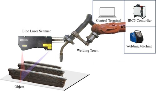
Table 1. Line-laser scanner parameters.

Model	Scan height	Scan X length	Z-axis accuracy	X-axis accuracy	Single line points
SR7400	200mm	240mm	5μm	90μm	3200

The coordinate system for the point cloud data is determined by the acquisition process of the scanner. The origin is defined in this coordinate system as the first point acquired by the scanner at the start of the acquisition. The X-axis is aligned with the laser line emitted by the scanner, while the Y-axis corresponds to the scanner's movement path, which is expected to be a straight line during the acquisition. The height information is represented via the Z-axis, which is aligned with the deposition direction. Therefore, the Z-coordinate value indicates the height of the scanned surface.

3. Method

3.1 Detection objective

Despite the implementation of various control measures, defects are still inevitable in WAAM process due to the long deposition time and complex nonequilibrium thermodynamics involved. The susceptibility of materials to defects such as cracks, deformations, pores, bulges, and humps varies.

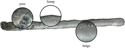
There are three specific types of defects common in WAAM: pores, bulges, and humps. Process anomalies, external disturbances, temperature, and material distribution within the molten pool are all factors that influence these defects [29,30]. Analysis of the 3D point cloud of weld beads revealed distinct geometric features associated with these three types of defects. Pores and bulges exhibit significant curvature, whereas hump defects display noticeable distortion in terms of height and width. The detection system will compute and use these distinguishing features to find out the defects efficiently. Figure 2 illustrates the morphological features of these three types of defects observed on the weld bead.

Figure 2. Defect detection objective.

3.2 System processes

Based on the geometric features of defects, a defect detection and evaluation system has been developed. The system, as shown in Figure 3, consists of four modules: weld bead extraction, hump detection, pore and bulge detection, and defect evaluation.

Figure 3. Processes of defect detection and evaluation system.

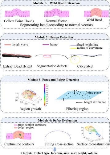
The weld bead extraction process seeks to minimize the influence of the substrate, improve detection accuracy and efficiency, and concentrate on defect detection and evaluation on the weld bead surface. Hump defect detection involves analysing the weld bead height curve along the centreline, and considering both 2D curvature and height discrepancy. After capturing the raw point cloud image with the camera, the statistical outlier filter is used to remove noise from the image. This algorithm is a common noise removal algorithm in point cloud processing, and has a good effect on the noise point cloud processing [28]. The 3D curvature of the point cloud is used to detect pore and bulge defects. A region-growing approach is used to locate areas of high-curvature to segment defects. The resulting segmented areas are then filtered and classified to enable efficient defect detection. For defect evaluation, a polynomial fitting model is used to fit the cross-sectional contours of the weld bead. This model allows the defect evaluation module to predict and reconstruct the normal weld bead contour within the defect area. The severity of the defect is assessed quantitatively by comparing the original and reconstructed surfaces.

3.3 Weld bead extraction

3.3.1 Computing normal vector

Normal vectors and curvatures are essential for analysing the geometric features of point clouds, such as segmentation, classification, and feature detection. A higher curvature value indicates a more pronounced curvature of the surface at that particular point within the point cloud. These measurements provide valuable information regarding the local surface orientation and shape. The computation of local surface property attributes is based on the examination of surrounding points. Commonly known as the k-nearest neighbour denoted by $N_P$. Typically, eigenanalysis of the covariance matrix of a local neighbourhood can be used to estimate local surface properties including normal vector and surface curvature [32].

For a given point $p_i=\left(x_i,y_i,z_i\right)$,the covariance matrix $\mathit{C}$ is defined as follows: (1) $\mathit{C}={\left[\begin{array}{c}{p}_{i_1}-\overline{p}\\ \cdots \\ p_{i_k}-\overline{p}\end{array}\right]}^T\cdot \left[\begin{array}{c}{p}_{i_1}-\overline{p}\\ \cdots \\ p_{i_k}-\overline{p}\end{array}\right],i_j\in N_p$(1) where $\overline{p}$ is the centroid of the neighbours of $N_P$, $p_{i_j}$is the j^th neighbour point of $p_i$.

Singular value decomposition is performed on the covariance matrix $\mathit{C}$ to obtain eigenvalues ${\lambda }_l({\lambda }_0<{\lambda }_1<{\lambda }_2)$. Their corresponding eigenvectors are $v_l(v_0,v_1,v_2)$. The eigenvectors can be obtained by solving the eigenvector problem shown in Equation (2). (2) $\mathit{C}\cdot v_l={\lambda }_l\cdot v_l,l\in \left\{0,1,2\right\}$(2) In this work, the eigenvector $v_0$ with the smallest eigenvalue ${\lambda }_0$is used as the estimated normal vector ${\mathit{n}}_i$ at point $p_i$. (3) ${\mathit{n}}_i=v_0$(3)

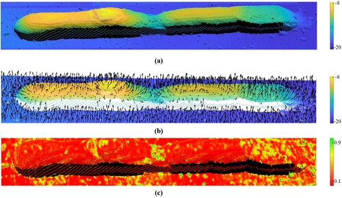
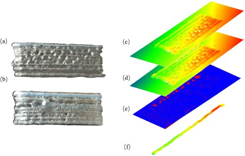
And surface curvature $\sigma$ is estimated by calculating between the eigenvalues of the covariance matrix: (4) $\sigma \left(p_i\right)={\displaystyle \frac{{\lambda }_0}{{\lambda }_0+{\lambda }_1+{\lambda }_2}}$(4) The calculation of local surface properties (normal vector and surface curvature) was based on the method in reference [31]. Functions in PCL were used in the program. The detailed derivation and computational procedure can be found in [30,31]. Figure 4 displays the results of normal vector and curvature computations based on the analysis of the point cloud of a deposition case. Figure 4a presents the original 3D point cloud dataset. Figure 4(b,c) exhibit the normal vectors extracted from the feature vector set and the computed curvature values determined by Equation (4), respectively. The curvature values at each point within the point cloud are marked with distinct colours to represent variations in curvature. As discussed above, defect areas pores, bulges and humps show larger curvature than their surrounding, the curvature was used distinguishing feature to identify the defects. In Figure 4c, the green areas are likely to be defect areas.

Figure 4. The curvature and normal vector of the point cloud; (a) 3D point cloud; (b) normal vector of point cloud; (c) curvature of the point cloud.

3.3.2 Segmenting weld bead

The segmentation of the weld bead area is determined by the significant distinction between the normal vectors of the weld bead and the background. Since the weld bead can vary, also vary the normal vectors in the X and Y directions. Therefore, the Z-component of the normal vector is used for weld bead segmentation. The 3D normal vector information is first converted into a 2D grayscale image. Each point in the point cloud will be assigned a pixel index based on its X and Y coordinates, and the corresponding pixel value is determined by the Z-component of the normal vector. The conversion formula is as follows: (5) $I_x={\displaystyle \frac{x_i-X_0}{d_x}}$(5) (6) $I_y={\displaystyle \frac{y_i-Y_0}{d_y}}$(6) (7) $M\left(I_x,I_y\right)=n_{iz}\cdot 255$(7) Where:$x_i,y_i$ represent the X and Y coordinates of the i-th point in the point cloud,

$X_0$,$Y_0$ are the minimum values of the entire point cloud sequence in the X and Y directions,

$I_x$,$I_y$ are the pixel indices of the i-th point on the two-dimensional image,

$d_x$,$d_y$ are the lengths of each point in the X and Y directions in the point cloud, with specific values determined by the camera settings during acquisition,

${\mathit{n}}_{iz}$ represents the Z-component of the normal vector of the point.

The applied example in Figure 5 is translated into a 2D grayscale image using the aforementioned conversion procedure, as illustrated in Figure 5a. An image segmentation algorithm is used to extract the weld bead region. As shown in Figure 5, the method comprises morphological operations such as threshold segmentation, erosion, dilation, opening, and closing, as well as contour processing.

Figure 5. Weld bead extraction process, (a) normal vector Z-component two-dimensional graph; (b) segmentation threshold of 240; (c) closed operation; (d) extracted weld bead contour; (e) removal of noise around the contour based on contour area; (f) opening and closing operation.

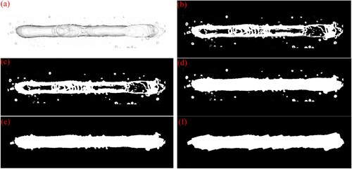
After successfully separating the weld bead region from the substrate in the 2D grayscale image (Figure 5f), the next step was to generate the corresponding 3D point cloud of the weld bead region. This was accomplished by performing an inverse calculation with Equations (5) and (6), which allowed the extraction of the weld bead in the 3D point cloud. By performing the weld bead segmentation procedure, the data size is reduced significantly, facilitating more accurate and efficient defect detection.

3.4 Humps detection

Humps, as defined in Section 3.1, are areas in the weld bead that have rapid fluctuations in both height and width along the centreline. Humps are detected by employing two fundamental elements of the height curve: the height difference and the 2D curvature of the height curve.

3.4.1 Extracting the centreline

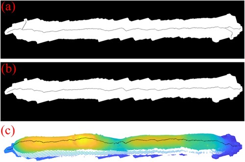
First, the weld bead height curve is defined as the curve corresponding to the geometric centreline of the two-dimensional weld bead contour. Because of its faster processing speed and robustness, the morphological thinning method is preferred over other methods for calculating the centreline. According to the algorithm proposed by Zhang et al. [33], the excess branches generated after thinning have been eliminated based on their lengths, resulting in the centreline of the weld bead contour. Finally, the corresponding three-dimensional points are determined using Equations (5) and (6).

Figure 6 depicts the process of extracting the centreline of the weld bead profile. Figure 6a shows the centreline produced through morphological thinning. The final centreline was obtained by eliminating specific branches, as shown in Figure 6b. The corresponding centreline point cloud (Figure 6c) was obtained by mapping the relationship between the 3D and 2D representations.

Figure 6. Extraction process of weld bead centreline; (a) result of morphological thinning; (b) the simplified centreline; (c) the centreline in the 3D point cloud.

3.4.2 Computing height curve features

As previously stated, the height curve along the centreline was used in this investigation, and humps were detected using two features of the height curve: height difference and 2D curvature. To compute these features, the points on the centreline of the 3D weld bead must be transformed into a 2D curve that describes the height of the weld bead. The following is the transformation formula: (8) ${\mathrm{X}}_i={\mathrm{X}}_{i-1}+\sqrt{{\left(x_i-x_{i-1}\right)}^2+{\left(y_i-y_{i-1}\right)}^2}i>0$(8) (9) ${\mathrm{Y}}_i=z_i$(9) where ${\mathrm{X}}_i$ and ${\mathrm{Y}}_i$ are the coordinates of the transformed two-dimensional height curve with ${\mathrm{X}}_0=0$, ($x_i,y_i,z_i$) is a point on the centreline.

The height difference is the discrepancy between the actual and theoretical heights. The theoretical height of the weld was determined using the Random Sample Consensus (RANSAC). For straight welds, the algorithm employed linear regression to fit a straight line, while for curved welds, it utilized a plane fitting method. The procedure of fitting a line using the RANSAC algorithm is illustrated in Table 2.

Table 2. RANSAC line fitting algorithm summary.

RANSAC Line Fitting Algorithm
1	Select two random points to determine the line
2	Solve the coefficients of the line
3	Calculate how many of the original points meet the requirement for a given tolerance and save the number of points that meet the requirement
4	Judge whether the prescriptive requirements are met. If the requirements are met, save the corresponding coefficient values. Otherwise, compare the existing points with the optimal solution and then store the best coefficient values as well as the coordinates of the data points.
5	Repeat the above steps for a given number of cycles

The curvature of the weld bead height curve is referred to as 2D curvature. Each point along the height curve determines its curvature by calculating the reciprocal of the radius of a fitted circle. The radius of the circle is calculated by the least square method fitting.

3.4.3 Segmenting hump defect area

As shown in Equation (10), a combined index $f$ was defined to indicate the location of the hump defects, taking into consideration both the height difference and the 2D curvature. (10) $f\left(i\right)=\alpha h_i+{\displaystyle \frac{\text{β}}{R_i}}$(10) where $\alpha$ and $\text{β}$ are coefficients, $h_i$ is the height difference, and $R_i$ is the curvature radius of the height curve. After many tests and experimental verification, it was found that the curve of the combined index shows sufficient prominent features to indicate hump defects when $\alpha$ is set to 1 and $\text{β}$ is set to 20.

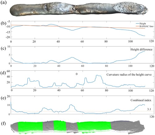
An example of hump defect detection is shown in Figure 7. Figure 7b presents the curves of the real height and theoretical height, and their height difference is shown in Figure 7c. Figure 7d shows the 2D curvature radius of the height curve. Figure 7e demonstrates the curve of the combined index. With experiments and adjustments to test cases, 3.1 is finally determined as the threshold of comprehensive evaluation. The area where the combined index value is above the segmentation threshold of 3.1 is believed to be the hump area. And in Figure 7f the corresponding areas are marked as hump defects.

Figure 7. Humps defect detection; (a) image of weld bead; (b) the real height curve and RANSAC fitted line; (c) height difference; (d) curvature radius of the height curve; (e)the combined index; (f) result of hump detection.

3.4.4 Test failure cases and reasons

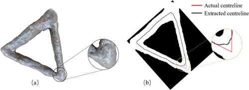
The proposed hump detection method encountered difficulty in some special cases. In the case shown in Figure 8, the deposited component has sharp corners. At the corners, the extracted centreline deviates from the real centreline to inner side. Since the height curve along the centreline was used to detect humps, the deviation of centreline around the corner would cause failure to detect humps if exist. From the magnification view in Figure 8a, there was a small hump around the corner, but the system failed to detect it. Meanwhile, if the centreline deviation is very large, a normal corner could be wrongly detected as hump. The ability of the system to treat deposition with sharp corners needs to be improved.

Figure 8. Detection failure case: (a) Triangular deposition; (b) Extracted centreline and actual centreline.

3.5 Pores and bulges detection

Because pore and bulge areas had greater 3D curvature than surrounding parts, a region-growing algorithm was utilized to segment high-curvature regions, and the segmented regions were subsequently filtered to discover defects.

3.5.1 Regional growing

The region-growing segmentation of the point cloud was performed using PCL's method [31]. This library furnishes an extensive array of tools and algorithms meticulously tailored for the processing and analysis of point cloud data. The process involved selecting the seed set based on the smallest curvature point and its normal vector. Subsequently, neighbouring points were thoroughly inspected, and those whose angles concerning the current seed's normal fell below the specified threshold were incorporated into the present region. If the curvature of the adjacent point was also below the threshold, it was added to the seed set, and the current seed was removed. The used threshold values are the optimal choice based on the comparison between detection results and manual measurement results. This iterative process persisted until the seed set was depleted, signifying the completion of region growth.

3.5.2 Filtering region

Following the region-growing segmentation, the potential defect areas exhibiting notably high 3D curvatures can be obtained. However, due to the intrinsic surface roughness of parts produced by WAAM, misidentification of normal regions as defects are possible. To mitigate this issue, a height filtering technique is implemented to eliminate areas where the impact of defects is minimal.

To begin, a 3D plane is fitted using the least-squares approach to each region's point cloud produced by region growth. Then compute distance of each point in the point cloud from the plane, if the point is above the fitted plane, the distance is positive; otherwise, it's negative. Finally, calculate the maximum height difference of the region's point cloud relative to the fitted plane, which is the difference between the maximum and minimum distances, and regions with small distance differences are removed.

Figure 9 shows an example of pore and bulge detection. The potential defect regions after the region growth are shown in Figure 9a. After filtering the regions with minor differences in height, the results are displayed in Figure 9b.

Figure 9. Regional growth segmentation and filtering region.

The filtered regions are considered as areas where pore or bulge defects exist. To discern the defect type more effectively, the correlation between the defect surface and the normal weld bead surface is leveraged. The specific implementation details are described in Section 3.6.3.

3.6 Defect evaluation

The defect evaluation module utilized a polynomial fitting model to accurately fit the cross-sectional contours of the weld bead. The proposed model predicts and reconstructs the normal weld bead contour in regions containing defects, subsequently conducting a quantitative assessment of defect severity through a comparative analysis of the actual and predicted surface disparities.

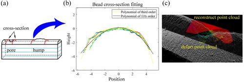
3.6.1 Acquiring cross-section

A comprehensive grasp of the normal cross-sectional contour of the weld bead is required to accurately rebuild the point cloud of the weld surface in the defective region. This approach encompasses the extraction of cross-sectional point clouds surrounding the defect and the establishment of correspondences between the 2D and 3D representations to obtain the point cloud data for the cross-section. To improve accuracy, five cross-section profiles are extracted from each end of the defect to determine the contour model (Figure 10a).

Figure 10. Defect evaluation process; (a) extraction of the weld bead cross-section; (b) polynomial fitting; (c) surface reconstruction of the defect.

The point cloud $P_c$ of each cross-sectional weld was processed using Equation (11) and (12) to convert it into a 2D point set. (11) ${\mathrm{X}}_i=\sqrt{{\left(x_i-x_0\right)}^2+{\left(y_i-y_0\right)}^2}\cdot fla{g}_i,i\in P_c$(11) (12) ${\mathrm{Y}}_i=z_i-z_0,i\in P_c$(12)

Where $x_i$, $y_i$, $z_i$ are the coordinates of the i-th point on the extracted cross-section profiles, and $x_0$, $y_0$, $z_0$ are the coordinates of the intersecting point of the centreline and the cross-section profile. The side of the point on the centreline is denoted by $fla{g}_i$, where −1 represents the left side and +1 represents the right side, respectively. The points on the cross-section were transformed, as shown in Figure 10b.

3.6.2 Polynomial fitting

The contour model of the weld cross-section was established using polynomial functions. Initially, the weld bead cross-section was fitted with a second-order polynomial, and the error between the fitting function and contour points was evaluated. If the error is within an acceptable range, the second-order polynomial is deemed the representation of the contour model. Nevertheless, when the error exceeds the permissible range, a higher-order polynomial, such as a third-order polynomial, is utilized as an alternative approach. This iterative process continues until a polynomial that satisfies the error criteria is found.

The polynomial fitting process is as follows. Assuming that there are n points in the transformed cross-sectional contour data and that an m-order polynomial is used to fit the data, the fitting function is given by. (13) $f\left({\mathrm{X}}_i\right)=a_m{\mathrm{X}}_i^m+a_{m-1}{\mathrm{X}}_i^{m-1}+\cdots +a_1{\mathrm{X}}_i+a_0$(13) Where $a_0$, $a_1$, … $a_m$ are polynomial coefficients, their values are determined by fitting cross-sectional data using the least-squares method. The results of fitting the contour points of the weld cross-section with third-order and fifth-order polynomials are shown in Figure 10b.

3.6.3 Weld bead surface reconstruction

The theoretical surface point cloud of the weld bead was reconstructed based on the theoretical height after the contour model of the weld bead was obtained. For each defective area, the theoretical height${\mathrm{z}}^{{}^{\mathrm{\prime }}}$should be calculated with the X and Y coordinates unchanged as follows: (14) ${\mathrm{z}}^{\mathrm{\prime }}={\mathrm{z}}_{\mathrm{t}\mathrm{h}}+f\left({\mathrm{X}}_i\right)$(14) Where ${\mathrm{X}}_i$ represents the distance between points calculated using Equation (11) and the centreline, whereas ${\mathrm{z}}_{\mathrm{t}\mathrm{h}}$ denotes the theoretical height of the point on the centreline in the weld cross-section, which was computed in Section 3.4.2. The reconstructed weld bead surfaces and defects are shown in Figure 10c.

If a defective region is confirmed as a pore or bulge defect during the detection process, the type of defect is determined based on the spatial relationship between the predicted point cloud and the defective point cloud. Defective point clouds that were located below the predicted point cloud were classified as pore defects, whereas those located above it were classified as bulge defects.

3.6.4 Calculating defect parameters

Several geometric parameters of the defects, including the area (A), volume (V), and elevation (E), were calculated for quantitative evaluation of the defects’ severity. These parameters were computed by comparing the reconstructed weld bead point cloud to the real defect point cloud.

The formula for computing A is as follows: (15) $A=A_0\ast Sum\left(Px\right)$(15) where$A_0$ is the area of the unit pixel, $Sum\left(Px\right)$ is the total number of pixels of the defective area.

The volume of each defect is calculated as follows: (16) $V=\sum _{i=1}^n\left|z_i^{{}^{\mathrm{\prime }}}-z_i\right|\ast A_0$(16) The elevation of each defect is calculated as follows: (17) $E=max\left\{\left|z_i^{{}^{\mathrm{\prime }}}-z_i\right|\right\}$(17)

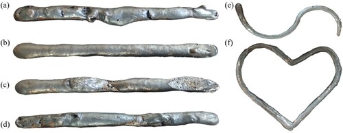
4. Case analysis

To assess the performance of the proposed defect detection system in real production scenarios, several thin-walled parts were deposited by WAAM in a multi-layer style. Defects on the surface of each part were purposefully created by utilizing aberrant welding procedures or conditions. Figure 11 shows some of the test cases.

Figure 11. Test cases.

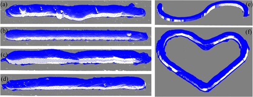
4.1 Weld bead extraction results

The results of weld bead extraction are presented in Figure 12, with the blue regions representing the weld beads of interest. The results demonstrated that weld beads of various shapes may be segmented while preserving the integrity of the point cloud utilizing the normal vector and morphology technique. All these cases demonstrate that the proposed extraction method can achieve fast extraction of weld beads of complex shapes in WAAM and has very strong resistance to interference beyond the regions of interest.

Figure 12. Result of weld extraction.

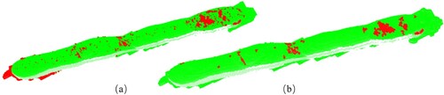
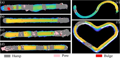
4.2 Defect detection results

The defect detection results for these test cases are presented in Figure 13, where the grey area represents humps, red represents bulges, and pink represents pores. By comparing Figure 11 and Figure 13, the following conclusions can be drawn: (1) all macroscopic defects of pores, bulges, and humps have been successfully detected with high accuracy; (2) two types of defects have been detected overlapping in some areas (bulges in the hump area, or pores in the hump area), which proved the ability of the proposed method. However, it is very difficult to detect defects with geometries that are not in the measuring accuracy range of line-laser scanners, such as crack defects.

Figure 13. Result of defect detection.

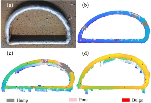
In the actual production process of WAAM, the deposited weld bead should be detected after each layer of deposition, thereby performing whole-time in-situ quality control of the WAAM process. In the process of multi-layer deposition, the system can detect defects during the deposition of each layer Figure 14 presents an example of multi-layer deposition and its interlayer detection results. The results of defect detection on the second, fourth, and ninth layers are depicted in Figure 14, which demonstrates the accurate identification of the defect location and type.

Figure 14. Detection results of interlayer accumulation; (b) The results of defect detection on the second layer; (c) The results of defect detection on the fourth layer; (d)The results of defect detection on the ninth layer.

The test case comprised 30 straight and 10 curved weld beads. Manual inspection detected 57 hump defects, 573 porosity defects, and 244 bulge defects, Table 3 presents the detection results. Table 4 shows the calculated point cloud scale and the computation time under the current hardware platform (Intel(R) Core(TM) i7-7700 and NVIDIA GeForce GTX 745).

Table 3. Defect detection result.

Real type	Algorithm detection result				Summary
	Normal	Pore	Bulge	Hump
normal	–	13	9	3	25
pore	38	512	23	0	573
bulge	9	18	217	0	244
hump	4	0	0	53	57

Table 4. Time statistics of normal and curvature are calculated.

Case No.	Deposition type	Defect quantity			Point cloud scale	Computation time(s)
		Humps	Pores	Bulges
Case A	A(line)	3	13	6	147181	13.33
Case B	A(line)	1	1	7	141930	6.83
Case C	A(line)	2	8	0	151479	8.54
Case D	A(line)	4	11	5	147409	12.36
Case E	A(curve)	0	7	3	476634	11.50
Case F	A(curve)	6	9	2	487246	11.54
Case G	B(curve)	2	4	3	514610	9.54
Case H	C(line)	2	6	4	72048	8.30

Notes: Deposition type, A: Single-layer single-bead deposition; B: Multi-layer single-bead deposition; C: Multi-layer multi-bead deposition.

In the Case H as shown in Figure 15, multi-layer multi-bead (3 layers × 9 beads) deposition was performed. During the entire process, the deposited component was scanned after every bead of deposition. For this case, there were 27 beads of deposition in total. By overlapping the point clouds of the current state and the state after previous bead deposition, the point cloud of the current bead can be obtained, which is a single-bead point cloud. Subsequently, the detection and evaluation were performed to the current bead in the same way as illustrated in Section 3.4-3.6. As shown in Figure 15, the morphology after the first layer (contain 9 beads, Figure 15a) and after the first bead of the second layer (contain 10 beads, Figure 15b) were both scanned. The point cloud of the 10th bead was obtained by overlapping the two datasets of point cloud provided by laser scanner.

Figure 15. (a) After the first layer; (b) After the first bead of the second layer; (c) point cloud image of (a); (d) point cloud image of (b); (e) Overlapping of (a) and (b), blue for (a), red for (b); (f) Extracting the point cloud of current bead to be detected.

Several measures, including accuracy, precision, recall, and F1 score, can be calculated to further assess the algorithm's performance. The formulas for these metrics are as follows: (18) $\{\begin{array}{c}Accuracy={\displaystyle \frac{TP+TN}{TP+TN+FP+FN}}\\ Precision={\displaystyle \frac{TP}{TP+FP}}\\ Recall={\displaystyle \frac{TP}{TP+FN}}\\ F1=2\times {\displaystyle \frac{Precision\ast Recall}{Precision+Recall}}\end{array}$(18) Where:

TP (True Positive) represents the number of correctly predicted positive samples.

TN (True Negative) represents the number of correctly predicted negative samples.

FP (False Positive) represents the number of incorrectly predicted positive samples.

FN (False Negative) represents the number of incorrectly predicted negative samples.

Table 5 presents the calculation results of these evaluation metrics.

Table 5. Evaluation metrics of the algorithm.

	Accuracy	Precision	Recall	F1
Pore	–	94.3	89.4	91.8
Bulge	–	87.1	88.9	88.0
Hump	–	94.6	93.0	93.8
Summary	90.5	92.0	90.4	91.2

The results demonstrate that the proposed defect detection algorithm effectively detects a majority of surface defects and accurately classifies them. The findings illustrate the efficacy of the proposed defect detection algorithm in identifying a significant portion of surface defects while precisely categorizing them.

The diminished accuracy in defect detection can be attributed to the clustering of porosity or protrusion defects during region segmentation, leading to the aggregation of multiple defects being treated as a single region. This, in turn, reduces the success rate of defect classification. However, when considering solely the probability of detecting defects, the success rate is 94.7%.

Remarkably, the probabilities of misidentifying pore and bulge defects as normal areas were observed to be 6.63% and 3.95%, respectively. The structural features of the defective area are responsible for the significant discrepancy of 40.4%. Specifically, in the case of porosity, the rapid depression hinders the laser scanner from receiving reflected light, resulting in the loss of local information and a drop in detection accuracy.

4.3 Defect evaluation results

The defect evaluation module, as detailed in Section 3.6.4, may determine the geometric parameters of defects. To verify the accuracy of the parameters, a test was designed, as shown in Figure 16a. In real-world scenarios, the measurement of defect height and volume poses challenges due to their dependence not only on the physical properties of the defective surface but also on the theoretical surface. The methodology employed involves the simulation of humps and bulge defects by applying rubber putty onto a defect-free weld bead. This choice is based on the ease of measuring the elevation and volume of the rubber putty. In Figure 16a, the green rubber putty is utilized to represent the simulated defect.

Figure 16. Result of defect evaluation.

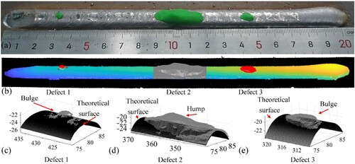
As shown in Figure 16b, the defect detection algorithm successfully identified the three simulated defects; defects 1 and 3 were identified as bulge defects, and defect 2 as humps. The theoretical surface was obtained using a surface reconstruction algorithm, which is represented by the black surface in Figure 16(c, d and e). Concurrently, the grey points in the figure may correspond to actual defective surfaces.

Upon completion of the scanning process, the simulated defects were captured in photographs, taken from both top and side orientations. Top-view photos were employed to quantify the areas of the simulated defects, whereas the side-view was used to measure the elevation. Subsequently, the rubber putties were removed from the weld bead and the volumes were measured. All the parameters obtained by manual and algorithmic measurements are presented in Table 6. A preliminary comparison of each parameter demonstrates that the algorithm yields a comparatively accurate evaluation of defects. The average discrepancies in the evaluation of elevation, area, and volume compared with manual measurements were 2.65%, 16.55%, and 5.03%, respectively. The error in the area is the largest. This is primarily attributed to the inclusion of some unrelated regions during the region growth process used for segmenting pores and bulges.

Table 6. Defect evaluation result.

	Algorithm measurement			Manual measurement
	Elevation (mm)	Area (mm^2)	Volume (mm^3)	Elevation (mm)	Area (mm^2)	Volume (mm^3)
Defect 1	1.69194	28.326	16.134	1.74	22	15.2
Defect 2	3.75626	405.834	495.468	3.68	380	460
Defect 3	1.43365	154.054	47.133	1.48	135	50
Error	2.65%	16.55%	5.03%	-	-	-

5 Conclusion

This research presents a surface defect detection and evaluation system designed for the WAAM process. The system effectively accomplishes the localization, classification, and quantitative severity evaluation of surface defects by analysing the geometric features of the weld bead point cloud. The following conclusions can be drawn from this study:

1. The feasibility of defect detection and severity evaluation through geometric features has been successfully demonstrated. The identification of hump defects relies on curvature calculation and height difference analysis, while the segmentation of pore and bulge defects is based on 3D curvature analysis. Experimental results demonstrate an accuracy of 90.5%, precision of 92%, and recall of 90.4%.

2. The quantitative analysis of defect severity is accomplished through a comparative examination of the point clouds derived from reconstructed normal weld surfaces and actual defects. Parameters such as defect area, elevation, and volume are calculated to facilitate this analysis. Defect simulation experiments indicate that the majority of errors fall within an acceptable range, except for relatively large area errors. These findings serve as a basis for subsequent defect handling.

3. The success rate of defect detection is intricately linked to the density and integrity of point clouds. Higher-density point clouds tend to result in higher success rates for detecting porosity and protrusion defects. Nevertheless, it should be noted that higher-density also leads to increased computational complexity.

The implemented system facilitates in-situ automatic defect detection within the WAAM process, offering continuous quality control and improving productivity. Nonetheless, a constraint of the system lies in its incapacity to detect small crack defects owing to the restricted precision of the line-laser scanner. To address this limitation, future efforts should concentrate on integrating supplementary sensors, such as CCD cameras and ultrasonic sensors, into the detection system. This integration would augment the system's defect detection capabilities and bolster its overall accuracy. Leveraging these advancements, the system has the potential to significantly diminish manufacturing failure rates, thereby contributing to enhanced overall productivity.

Disclosure statement

No potential conflict of interest was reported by the author(s).

Data availability statement

The data that support the findings of this study are openly available in Mendeley Data at doi: 10.17632/vm5rmhtxbx.1.

Additional information

Funding

This work was supported by the National Natural Science Foundation of China (grant number 51975270), Natural Science Foundation of Hunan Province (grant number 2023JJ30510), Key Project of Education Department of Hunan Province, China (grant number 21A0257).

References

- Chadha U, Abrol A, Vora NP, et al. Performance evaluation of 3D printing technologies: a review, recent advances, current challenges, and future directions. Progr Addit Manufact. 2022;7(5):853–886. doi:10.1007/s40964-021-00257-4
- Mehnen J, Ding J, Lockett H, et al. Design study for wire and arc additive manufacture. Intern J Prod Develop. 2014;19(1-3):2–20. doi:10.1504/IJPD.2014.060028
- Plocher J, Panesar A. Review on design and structural optimisation in additive manufacturing: Towards next-generation lightweight structures. Mater Des. 2019;183:108164), doi:10.1016/j.matdes.2019.108164
- Taşdemir A, Nohut S. An overview of wire arc additive manufacturing (WAAM) in shipbuilding industry. Ships Offsh Struct. 2021;16(7):797–814. doi:10.1080/17445302.2020.1786232
- Singh S, kumar Sharma S, Rathod DW. A review on process planning strategies and challenges of WAAM. Mater Today Proc. 2021;47:6564–6575. doi:10.1016/j.matpr.2021.02.632
- Mu H, He F, Yuan L, et al. Toward a smart wire arc additive manufacturing system: A review on current developments and a framework of digital twin. J Manufact Syst. 2023;67:174–189. doi:10.1016/j.jmsy.2023.01.012
- Zhu X, Jiang F, Guo C, et al. Surface morphology inspection for directed energy deposition using small dataset with transfer learning. J Manuf Process. 2023;93:101–115. doi:10.1016/j.jmapro.2023.03.016
- He F, Yuan L, Mu H, et al. Research and application of artificial intelligence techniques for wire arc additive manufacturing: a state-of-the-art review. Robot Comput Integr Manuf. 2023;82:102525), doi:10.1016/j.rcim.2023.102525
- Rout A, Deepak B, Biswal BB. Advances in weld seam tracking techniques for robotic welding: A review. Robot Comput Integr Manufact. 2019;56:12–37. doi:10.1016/j.rcim.2018.08.003
- Qin J, Hu F, Liu Y, et al. Research and application of machine learning for additive manufacturing. Addit Manufact. 2022: 102691), doi:10.1016/j.addma.2022.102691
- Shaloo M, Schnall M, Klein T, et al. A review of Non-destructive testing (NDT) techniques for defect detection: application to fusion welding and future wire Arc additive manufacturing processes. Materials (Basel). 2022;15(10):3697), doi:10.3390/ma15103697
- Vavilov VP, Pawar SS. A novel approach for one-sided thermal nondestructive testing of composites by using infrared thermography. Polym Test. 2015;44:224–233. doi:10.1016/j.polymertesting.2015.04.013
- Chen X, Zhang H, Hu J, et al. A passive on-line defect detection method for wire and arc additive manufacturing based on infrared thermography. International Solid Freeform Fabrication Symposium 2019. doi:10.26153/tsw/17375.
- Lopez A, Bacelar R, Pires I, et al. Non-destructive testing application of radiography and ultrasound for wire and arc additive manufacturing. Addit Manufact. 2018;21:298–306. doi:10.1016/j.addma.2018.03.020
- Xiong J, Zhang Y, Pi Y. Control of deposition height in WAAM using visual inspection of previous and current layers. J Intell Manuf. 2021;32:2209–2217. doi:10.1007/s10845-020-01634-6
- Xiong J, Pi Y, Chen H. Deposition height detection and feature point extraction in robotic GTA-based additive manufacturing using passive vision sensing. Robot Comput Integr Manuf. 2019;59:326–334. doi:10.1016/j.rcim.2019.05.006
- Cho HW, Shin SJ, Seo GJ, et al. Real-time anomaly detection using convolutional neural network in wire arc additive manufacturing: molybdenum material. J Mater Process Technol. 2022;302:117495), doi:10.1016/j.jmatprotec.2022.117495
- Wu J, Huang C, Li Z, et al. An in situ surface defect detection method based on improved you only look once algorithm for wire and arc additive manufacturing. Rapid Prototyp J. 2023;29(5):910–920. doi:10.1108/RPJ-06-2022-0211
- Li W, Zhang H, Wang G, et al. Deep learning based online metallic surface defect detection method for wire and arc additive manufacturing. Robot Comput Integr Manuf. 2023;80:102470), doi:10.1016/j.rcim.2022.102470
- Tang S, Wang G, Zhang H. In situ 3D monitoring and control of geometric signatures in wire and arc additive manufacturing. Surf Topogr Metrol Propert. 2019;7(2):025013), doi:10.1088/2051-672X/ab1c98
- Huang C, Wang G, Song H, et al. Rapid surface defects detection in wire and arc additive manufacturing based on laser profilometer. Measurement ( Mahwah N J). 2022;189:110503), doi:10.1016/j.measurement.2021.110503
- Chen X, Fu Y, Kong F, et al. An in-process multi-feature data fusion nondestructive testing approach for wire arc additive manufacturing. Rapid Prototyp J. 2021;28(3). doi:10.1108/RPJ-02-2021-0034
- Chaekyo L, Gijeong S, Bong DK, et al. Development of defect detection AI model for wire + arc additive manufacturing using high dynamic range images. Appl Sci. 2022;28(3):573–584. doi:10.1108/RPJ-02-2021-0034
- Lyu J, Manoochehri S. Online convolutional neural network-based anomaly detection and quality control for fused filament fabrication process. Virtual Phys Prototyp. 2021;16(2):160–177. doi:10.1080/17452759.2021.1905858
- Zhang Y, Yuan L, Liang W, et al. 3D-SWiM: 3D vision based seam width measurement for industrial composite fiber layup in-situ inspection. Robot Comput Integr Manuf. 2023;82:102546), doi:10.1016/j.rcim.2023.102546
- Samie Tootooni M, Dsouza A, Donovan R, et al. Classifying the dimensional variation in additive manufactured parts from laser-scanned three-dimensional point cloud data using machine learning approaches. J Manufact Sci Eng. 2017;139(9):091005), doi:10.1115/1.4036641
- Lin W, Shen H, Fu J, et al. Online quality monitoring in material extrusion additive manufacturing processes based on laser scanning technology. Precision Eng. 2019;60:76–84. doi:10.1016/j.precisioneng.2019.06.004
- Chen L, Yao X, Xu P, et al. Rapid surface defect identification for additive manufacturing with in-situ point cloud processing and machine learning. Virtual Phys Prototyp. 2021;16(1):50–67. doi:10.1080/17452759.2020.1832695
- Wu B, Pan Z, Ding D, et al. A review of the wire arc additive manufacturing of metals: properties, defects and quality improvement. J Manuf Process. 2018;35:127–139. doi:10.1016/j.jmapro.2018.08.001
- Yuan L, Pan Z, Ding D, et al. Investigation of humping phenomenon for the multi-directional robotic wire and arc additive manufacturing. Robot Comput Integr Manuf. 2020;63:101916), doi:10.1016/j.rcim.2019.101916
- Rusu RB, Cousins S. 3d is here: Point cloud library (PCL). IEEE international conference on robotics and automation. IEEE International Conference on Robotics and Automation. 2011: 1–4. doi:10.1109/ICRA.2011.5980567.
- Pauly M, Gross M, Kobbelt LP. Efficient simplification of point-sampled surfaces. Visualization (Los Alamitos Calif). 2002: 163–170. doi:10.1109/VISUAL.2002.1183771
- Zhang TY, Suen CY. A fast parallel algorithm for thinning digital patterns. Commun ACM. 1984;27(3):236–239. doi:10.1145/357994.358023