Numerical modelling of the viscoelastic polymer melt flow in material extrusion additive manufacturing

ABSTRACT

In material extrusion (MEX), it is challenging to accurately predict the steady and transient feeding forces at various polymer extrusion rates when printing island and thin-walled structures involving rapid start/stop or acceleration/deceleration, especially for semi-crystalline polymers. This research presents a non-isothermal viscoelastic Computational Fluid Dynamics model to investigate the steady and transient feeding forces, as well as the phase transition process and viscoelastic behaviour of polylactic acid (PLA), a semi-crystalline polymer, during the extrusion process. The study establishes a relationship between polymer flow and viscoelastic stress, demonstrating that the elastic effect during extrusion is more significant than the viscous effect, particularly at higher feeding rates. Furthermore, the study uncovers critical aspects of PLA melt flow behaviour during the MEX process, laying the foundation for future research and optimisation of MEX printing processes.

KEYWORDS:

• Material extrusion
• melt flow
• viscoelastic behaviour
• semi-crystalline
• feeding force prediction

1. Introduction

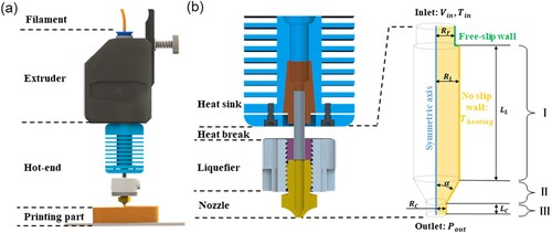
Fused Filament Fabrication, also known as Fused Deposition Modelling (FDM), is a material extrusion additive manufacturing technology proposed by Crump in 1986 [1] that builds parts layer by layer by melting and extruding filaments through the hot-end (Figure 1 (a)). The hot-end, responsible for melting and extruding the polymer filament, comprises a liquefier that transfers heat to polymers and an extrusion nozzle that deposits the melt onto the substrate, thereby constructing three-dimensional objects [2]. A profound understanding of melt flow evolution during printing is crucial for comprehending the limitations of the FDM process and optimising both the process and structure. Nevertheless, conducting a comprehensive analysis of the liquefier melting process and flow details using experimental techniques is challenging due to the difficulties involved in integrating in-situ measurement instruments within the hot-end. Consequently, numerous studies have extensively explored the melt flow behaviour of the filament in the hot-end through Computational Fluid Dynamics (CFD) methods.

Figure 1. (a) Schematic of FDM process; (b) Geometry of the hot-end channel and boundary conditions of the computational model.

The numerical research on the melting flow in the extrusion process of FDM mainly focuses on the following two aspects. One is to investigate the mechanism of melt flow in the hot-end of the FDM extrusion process [3–15], such as simulating the velocity, pressure, and temperature fields in the hot-end affected by the variation of different factors (e.g. heat transfer conditions, feeding rate, and material properties). The mechanical properties of printing parts hinge on the diffusion of the polymer chains at the interfaces formed during the extrusion and deposition processes [16–18], and this diffusion corresponds to the changes in physical fields, such as the velocity and temperature of the melt flow in the hot-end. The other research interest is predicting the feeding force during the printing process, i.e. the resistance that filament overcomes [3,4,7–9,19]. These studies aim to optimise the design of the hot-end to accommodate different working conditions, including high-speed printing, large-scale printing, and soft material printing. In each of these scenarios, it is crucial to continuously improve the model for higher computation accuracy and optimise the hot-end design to meet the printing requirement. Nevertheless, a notable discrepancy persists in predicting the steady-state feeding force under conditions of high feeding rates, elevated heating temperatures, small outlet diameters, and particularly for semi-crystalline polymers [4,7–9].

Most of the current numerical simulations are based on a generalised Newtonian fluid (GNF) constitutive model, which failed to consider the complete viscoelasticity of the polymer. The significance of considering viscoelasticity lies in the fact that the internal stresses also depend on their past deformations [20]. Moreover, it has been demonstrated that viscoelasticity significantly affects the conventional manufacturing processes for polymers, including injection/compression moulding, spinning, film blowing, and more [21–26]. Thus, characterising the polymer viscoelasticity in the FDM process becomes essential. Schuller et al. [27] conducted initial research on the viscoelastic behaviour of polymer fluids in the FDM process based on the assumption of isothermal flow with a nozzle of a unique geometry. Later, Serdeczny et al. established a non-isothermal flow viscoelastic model for the FDM extrusion process, but their research mainly focused on the prediction of steady-state feeding force [19]. However, for scenarios that require rapid start/stop or acceleration/deceleration of the extruder head, such as island structures and thin-walled structures, in-depth research on the transient feeding force changes during the printing process is yet to be explored. Also, most of the materials used in the above studies are amorphous polymers without a distinct melting point. However, semi-crystalline polymers, such as polylactic acid (PLA), have distinct melting points and enthalpy values. Thus, the viscoelastic flow mechanisms and their unique characteristics in transient response remain unexplored. Also, the impact of changes in empirical parameters in the phase transition model on viscoelastic melt flow needs to be further determined.

This study presents a non-isothermal viscoelastic CFD model to research the steady and transient feeding forces, the phase-transition process, and the viscoelastic melt-flow mechanism involved in the FDM extrusion process of semi-crystalline polymers. The model simulates the filament being heated and melted from a solid state to a liquid state and then extruded. The Giesekus model [28] is adopted to describe the viscoelastic behaviour of materials. The computational model with the enthalpy porosity method is then applied to semi-crystalline polymers (such as PLA), which exhibit a distinct melting point associated with the phase-transition process. Finally, simulations are performed to predict variations in transient feeding force in response to different velocity inputs, including step velocity and trapezoidal velocity profiles.

2. Methods and materials

2.1. Experimental and numerical instruments

All testing is performed with commercial PLA filament (Polymaker, China). A commercial FDM printer (INTAMSYS HT400) is used throughout this work, including feeding force measurements (more details in Appendix). All numerical simulations are conducted using ANSYS Fluent (ANSYS Inc., PA, USA), a commercial CFD software tool. The CFD model is solved based on the finite volume method within the software. To incorporate the viscoelastic constitutive model, a UDF (User Design Function) is developed using the C++ programming language.

2.2. Hot-end configurations and boundary conditions

Figure 1 (b) illustrates the fundamental configuration of a typical hot-end, consisting of the heat sink, heat break, liquefier, and nozzle. The liquefier is responsible for heating and melting the filament, which is then extruded through the nozzle for the layer-by-layer printing process. The heat break serves the purpose of blocking the upward heat flow from the liquefier, thereby preventing the polymer melt backflow to the low-temperature zone, This backflow could lead to the solidification of the polymer and blockage of the nozzle [29]. Furthermore, the heat sink effectively dissipates the heat transferred from below, ensuring that the filament maintains its shape and does not soften prematurely before reaching the liquefier. This facilitates the smooth entry of the filament into the liquefier.

Therefore, the primary focus of this study is the analysis of melt flow within the liquefier and nozzle sections during the FDM extrusion process. These sections implemented in the numerical model are divided into three zones, as illustrated in Figure 1 (b). The dimensions of the hot-end are summarised in Table 1. In addition, the boundary conditions (Figure 1 (b)) in this research are assumed as follows:

1. Considering the axisymmetry of the flow channel geometry, a two-dimensional axisymmetric model is established for the simulation, eventuating in a symmetric axis boundary condition.

2. The inlet boundary condition is defined as a velocity inlet with a given velocity and temperature, and the outlet boundary condition is set as a pressure outlet with a magnitude of one atmosphere.

3. Since there is a significant impact of the gap between the inlet filament and the liquefier wall in the simulations, and the gap-filling level will be maintained near the junction of the heat break and the liquefier [3,7,29], it is postulated that the filament wall at the heat break acts as a free-slip wall boundary condition. In other words, the filament does not contact the hot-end wall; instead, it replaces the interface between air and polymer.

4. The liquefier and nozzle contain the core region where the filament is melted and extruded. The wall of this region is assumed to have a constant heating temperature, representing a fixed wall boundary condition.

Table 1. Dimensions of INTAMSYS HT400 hot-end.

Dimension	Symbol	Value	Unit
Filament radius	${\mathit{R}}_{\mathit{F}}$	0.875	mm
Liquefier radius	${\mathit{R}}_{\mathit{L}}$	1	mm
Nozzle radius	${\mathit{R}}_{\mathit{C}}$	0.2	mm
Capillary length	${\mathit{L}}_{\mathit{C}}$	0.6	mm
Liquefier length	${\mathit{L}}_{\mathit{L}}$	20	mm
Contraction angle	$\mathit{\alpha }$	30	${}^{\circ }$

2.3. Governing equations of the CFD model

Under the defined conditions in Section 2.2, the governing equations used in our computational model are based on the research of Bird [30] and Bennon et al. [31]. The equations corresponding to volume, momentum, and energy balances are as follows: (1) $\begin{array}{c}\mathrm{\nabla }\cdot \mathit{u}=0,\end{array}$(1) (2) $\begin{array}{c}\rho {\displaystyle \frac{D\mathit{u}}{\mathrm{Dt}}=\mathrm{\rho g}+\mathrm{\nabla }\cdot \tau -\mathrm{\nabla p}-{\displaystyle \frac{\mu }{K}{\displaystyle \frac{\rho }{{\rho }_l}\left(\mathit{u}-{\mathit{u}}_{\mathit{s}}\right),}}}\end{array}$(2) (3) $\begin{array}{c}\rho C_p{\displaystyle \frac{\mathrm{DT}}{\mathrm{Dt}}=\kappa {\mathrm{\nabla }}^{2}T+\overline{\overline{\mathit{\tau }}}:\mathrm{\nabla }\mathit{u}-\mathrm{\nabla }\cdot \left(\rho f_{s}L\left(\mathit{u}-{\mathit{u}}_{\mathit{s}}\right)\right)-\mathrm{\rho L}{\displaystyle \frac{D{f}_l}{\mathrm{Dt}},}}\end{array}$(3) where $\mathit{u}$ is the velocity vector, ${\mathit{u}}_{\mathit{s}}$ is the solid push velocity vector corresponding to the filament feeding rate, $\rho$ is mixture density, ${\rho }_l$ is the fluid density, t is time, p is pressure, $\mathit{\tau }$ is the constitutive stress tensor, $g$ is the gravity vector, $C_p$ is the specific heat, T is the temperature, $\kappa$ is the thermal conductivity of the polymer, $\mu$ is the dynamic viscosity and L is the melting enthalpy. ${\displaystyle \frac{D}{\mathrm{Dt}}}$ is the substantial derivative, expressed as: ${\displaystyle \frac{D}{\mathrm{Dt}}={\displaystyle \frac{\mathrm{\partial }}{\mathrm{\partial }t}+\left(\mathit{u}\cdot \mathrm{\nabla }\right)}}$. In addition, $f$ is the mass fraction, while the subscript s and l represent the solid phase and liquid phase, which means $f_l+f_s=1$, as supplied as follows: (4) $\begin{array}{c}{f}_l=\{\begin{array}{c}0,\mathrm{if}T\le T_s\\ {\displaystyle \frac{T-T_s}{T_l-T_s},\mathrm{if}{T}_s<T<T_I}\\ 1,\mathrm{if}T\ge T_l\end{array},\end{array}$(4) where $T_l$ and $T_s$ represent the liquidus and solidus temperatures, respectively.

In Equations (1)–(3), the fluid is assumed to have a constant density, specific heat coefficient, and thermal conductivity. The material to be investigated is PLA, a widely used semi-crystalline polymer with distinct melting points and enthalpy values. Thus, it is essential to account for the phase change process that occurs within the polymer melt flow. Therefore, the corresponding source terms incorporated into the governing equations include: the fourth term ($-{\displaystyle \frac{\mu }{K}{\displaystyle \frac{\rho }{{\rho }_l}\left(\mathit{u}-{\mathit{u}}_{\mathit{s}}\right)}}$) on the right-hand side (RHS) of the momentum equation Equation (2); the third term ($-\mathrm{\nabla }\cdot \left(\rho f_{s}L\left(\mathit{u}-{\mathit{u}}_{\mathit{s}}\right)\right)$); and the fourth term ($-\mathrm{\rho L}{\displaystyle \frac{D{f}_l}{\mathrm{Dt}}}$) on the RHS of the energy equation Equation (3). These terms represent the Darcy force term, the interphase transfer term, and the latent heat term, respectively. The Darcy force term accounts for the flow of the liquid polymer through the porous mushy zone. The interphase transfer term in the energy equation describes the subsequent latent heat transfer. Lastly, the latent heat term represents the latent heat of fusion absorbed during the phase change of the polymer.

2.4. Constitutive model

The existing generalised Newtonian fluid models have reached their limits in accurately predicting extrusion flow behaviour. Therefore, it is imperative to consider the effects of material elasticity, especially when studying more complex transient fluid flows. Introducing a viscoelastic constitutive model is essential to provide a more precise description of polymer flow dynamics.

The Giesekus model [28] is applied as the constitutive model, which is related to the stress tensor term in Equations (2)–(3). The stress tensor term in the viscoelastic model can be expressed as follows: (5) $\begin{array}{c}\tau ={\mathit{\tau }}_{\mathit{s}}+{\mathit{\tau }}_{\mathit{p}},\end{array}$(5) where ${\mathit{\tau }}_{\mathit{s}}$ is the solvent stress term, i.e. the viscous stress due to polymer viscosity, and ${\mathit{\tau }}_{\mathit{s}}=2{\eta }_{\mathit{s}}\mathit{D}$, ${\eta }_{\mathit{s}}$ is the solvent contribution to the zero-shear rate viscosity ${\mathit{\tau }}_{\mathit{p}}$ is the stress contribution due to polymer elasticity; If for Newtonian fluids, ${\mathit{\tau }}_{\mathit{p}}=0$.

Next, the viscoelastic model is established to predict the polymer stress contribution ${\mathit{\tau }}_{\mathit{p}}$. To completely characterise the intricate viscoelastic properties of the polymer, a multi-mode formulation is adopted. Here, k is the mode number, i.e. the number of groups of constitutive equations. Thus, ${\mathit{\tau }}_{\mathit{s}}=\sum _{\mathit{k}=1}^{\mathit{n}}{\mathit{\tau }}_{\mathit{p}k}$. For a single-mode group, the Giesekus model can be expressed as follows: (6) $\begin{array}{c}{\mathit{\tau }}_{\mathit{p}k}+{\lambda }_k\stackrel{\mathrm{\nabla }}{{\mathit{\tau }}_{\mathit{p}k}}+{\alpha }_k{\displaystyle \frac{{\lambda }_k}{{\eta }_{\mathrm{pk}}}{\mathit{\tau }}_{\mathit{p}k}\cdot {\mathit{\tau }}_{\mathit{p}k}^T=2{\eta }_{\mathrm{pk}}D,}\end{array}$(6) where, ${\lambda }_k,{\alpha }_k,{\eta }_{\mathrm{pk}}$ are the relaxation time, mobility factor, and polymer viscosity for each mode k respectively. Meanwhile, $\stackrel{\mathrm{\nabla }}{{\mathit{\tau }}_{\mathit{p}k}}$ is the upper-convected derivative of the stress tensor for each mode defined as: (7) $\begin{array}{c}\stackrel{\mathrm{\nabla }}{{\mathit{\tau }}_{\mathit{p}k}}={\displaystyle \frac{D{\mathit{\tau }}_{\mathit{p}k}}{\mathrm{Dt}}-{\left(\mathrm{\nabla }u\right)}^T\cdot {\mathit{\tau }}_{\mathit{p}k}-{\mathit{\tau }}_{\mathit{p}k}\cdot \mathrm{\nabla u},}\end{array}$(7) where ${\displaystyle \frac{D{\mathit{\tau }}_{\mathit{p}k}}{\mathrm{Dt}}}$ is the substantial derivative of the stress tensor for each mode. In addition, the temperature dependence of the relevant parameters of the Giesekus model is characterised by the Arrhenius equation [32] as follows: (8) $\begin{array}{c}H\left(T\right)={\displaystyle \frac{{\eta }_0\left(T\right)}{{\eta }_0\left(T_0\right)}=\exp \left[{\displaystyle \frac{\mathrm{\Delta }H}{R_{\mathrm{ig}}}\left({\displaystyle \frac{1}{T}-{\displaystyle \frac{1}{T_0}}}\right)}\right],}\end{array}$(8) where H is the activation energy of flow, and $R_{\mathrm{ig}}$ is the ideal gas constant. The temperature dependence of rheological parameters is expressed as: (9) $\begin{array}{c}{\eta }_{\mathit{s}}=H\left(T\right){\eta }_{\mathit{s}0},\end{array}$(9) (10) $\begin{array}{c}{\lambda }_k=H\left(T\right){\lambda }_{k0},\end{array}$(10) (11) $\begin{array}{c}{\alpha }_k=H\left(T\right){\alpha }_{k0},\end{array}$(11) (12) $\begin{array}{c}{\eta }_{\mathrm{pk}}=H\left(T\right){\eta }_{\mathrm{pk}0}.\end{array}$(12)

In addition, the Cross model, which is a GNF model, is introduced for comparison. The Cross model is represented as follows: (13) $\begin{array}{c}\eta \left(\dot{\gamma }\right)={\displaystyle \frac{{\eta }_o^{\ast }}{\left[1+{\left({\lambda }^{\ast }\dot{\gamma }\right)}^{1-n}\right]},}\end{array}$(13) where $\eta \left(\dot{\gamma }\right)$, ${\eta }_o$, ${\lambda }^{\ast }$, and n are the shear viscosity, zero-shear viscosity, relaxation time, and the power-law index, respectively.

2.5. Material properties

In this study, a viscoelastic model is fitted by conducting a series of rheological experiments to identify quantities such as storage modulus, loss modulus, viscosity; and time-temperature equivalence. The modulus and viscosity of PLA are characterised using a HAAKE MARS 40 Rheometer (Thermo Fisher Scientific, US) with a set of 25 mm parallel plates, through the Small Amplitude Oscillatory Shear (SAOS) test. An amplitude scan is first performed at 453.2 K and 10 Hz to determine the strain within the linear viscoelastic region (LVR). The frequency scan ranging from 0.1 to 200 rad/s at 0.1 $\text{\%}$ strain amplitude is performed for 443.2, 453.2, 463.2, and 473.2 K. The SAOS test provided data that varied with the angular frequency ($\omega$). To obtain the shear rate ($\dot{\gamma }$) dependent viscosity model data, the Cox-Merz rule is applied, replacing the angular frequency with the shear rate. In addition, a reference temperature of 453.2 K is used.

Furthermore, the model fitting for parameter identification consists of two parts: one is to obtain the relaxation spectrum of the polymer melt’s linear viscoelasticity from the SAOS test. The other is to determine the values of the parameters α and $\mathrm{\Delta H}/R_{\mathrm{ig}}$ by fitting the nonlinear viscoelastic behaviour observed at various temperatures based on the relaxation spectrum.

For the Giesekus model, the relationship between the relaxation spectrum ($\lambda ,\eta$) and the experimental angular frequencies $\omega$, storage, and loss moduli $G^{\mathrm{\prime }}$ and $G{}^{\mathrm{\prime }}\mathrm{\prime }$ in the SAOS test can be expressed as: (14) $\begin{array}{c}{\mathrm{G}}^{\mathrm{\prime }}\left(\omega \right)=\sum _i{\displaystyle \frac{g_i{\lambda }_i^2{\omega }^2}{1+{\lambda }_i^2{\omega }^2},}\end{array}$(14) (15) $\begin{array}{c}{\mathrm{G}}^{{}^{\mathrm{\prime }}\mathrm{\prime }}\left(\omega \right)=\sum _i{\displaystyle \frac{g_i{\lambda }_i\omega }{1+{\lambda }_i^2{\omega }^2}.}\end{array}$(15) The experiments and model fitting are performed following the above procedures. The results are presented in Figure 2, which illustrates both the measured and fitted curves. The identified parameters can be found in Table 2.

Figure 2. (a) Fitted curve for storage and loss moduli $G^{\mathrm{\prime }}$ and ${\mathrm{G}}^{\mathrm{\prime \prime }}$. (b) Fitted curve for viscosity.

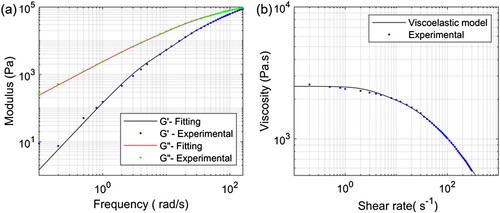
Table 2. Identified parameters for the constitutive model.

Viscoelastic Model
Parameter	Symbol	Unit	Value
			Mode 1	Mode 2	Mode 3
Mobility factor	${\alpha }_k$	–	0.609	0.794	0.485
Relaxation time	${\lambda }_{k0}$	$S$	0.0048	0.265	0.0249
Polymer viscosity contribution	${\eta }_{k0}$	$\mathrm{Pa}\cdot s$	615.1	965.4	987.1
Solvent viscosity contribution	${\eta }_{s0}$	$\mathrm{Pa}\cdot s$	131.4
GNF Model
Zero-shear viscosity	${\eta }_o$	$\mathrm{Pa}\cdot s$	2011.5
Relaxation time	${\lambda }^{\ast }$	$S$	0.014
Power-law index	$n$	–	0.26
Arrhenius Equation
Reference temperature	$T_0$	$K$	453.2
Activation energy/Gas constant	$\mathrm{\Delta H}/R_{\mathrm{ig}}$	$K$	10880

Additionally, modelling the material extrusion process requires the identification of the following parameters: density $\rho$, specific heat capacity $C_p$, thermal $\kappa$ conductivity, melting enthalpy L, liquidus, and solidus temperatures of the polymer. Liquidus and solidus temperatures remain constant, the other parameters are temperature-dependent. To simplify the simulation, only the temperature dependence of the parameters that significantly vary with temperature and have a prominent effect on the simulations have been considered, as shown in Table 3. The specific heat capacity with temperature for PLA from Phan et al. [9] can be transformed in Kelvin as follows: (16) $\begin{array}{c}{C}_P=\{\begin{array}{c}4.05T-760.45,T\le 428.15K\\ 2.42T-504.02,T>428.15K\end{array}.\end{array}$(16)

Table 3. Material properties adopted in the simulation.

Parameter	Symbol	Value	Unit	Source
Density	$\rho$	1.18	$g/c{m}^3$	[33]
Thermal conductivity	$\kappa$	0.2	$W/\mathrm{mK}$	[9]
Melting enthalpy	$L$	100	$J/g$	[9]
Solidus melting temperature	$T_s$	413.15	$K$	[9]
Liquidus melting temperature	$T_l$	428.15	$K$	[9]
Glass temperature	$T_g$	334.15	$K$	[33]

2.6. Phase transition model

In addition, the filament is heated and melted as it enters the liquefier, leading to a phase transition process from the solid to the liquid phase. The phase transition is commonly characterised in CFD through the enthalpy porosity technique proposed by Voller and Prakash [34]. While this model originated from the alloy solidification process, it has also been applied to the melting of crystalline or semi-crystalline organic materials [4,6,35–38] like paraffin and polylactic acid, yielding simulation results that align closely with experiments [4,35,39]. This technique treats the solid–liquid interface as an equivalent porous media, where the porosity represents the ratio of the latent heat content of the cells to the latent heat of fusion, and this phase transition interface is commonly referred to as the mushy zone. This method involves the identification of its empirical parameters, which have a significant impact on the melt flow simulation results [35,39,40].

The fourth term to the right-hand side of the momentum conservation equation Equation (2) and the third term to the right-hand side of the energy equation Equation (3) in the control equations reflect the use of the enthalpy porosity technique. The Darcy force term ${\mathit{S}}_{\mathit{F}}$ in Equation (2) is expressed in the simulation model as: (17) $\begin{array}{c}{\mathit{S}}_{\mathit{F}}=-{\displaystyle \frac{\mu }{K}{\displaystyle \frac{\rho }{{\rho }_l}\left(\mathit{u}-{\mathit{u}}_{\mathit{s}}\right).}}\end{array}$(17) where the permeability K is expressed according to the Kozeny-Carman equation. The equation is described as follows: (18) $\begin{array}{c}K={\displaystyle \frac{{\varphi }^3}{c{(1-\varphi )}^2{S}^2}.}\end{array}$(18) where c and S are the Kozeny-Carman constant and the specific surface area of the solid phase in the mushy zone, $\varphi$ is the porosity of the porous media, corresponding to the liquid fraction $f_l$, which means $\varphi =f_l$.

Since the polymer has been assumed to be an incompressible fluid during the FDM extrusion process for simulation, the density of the polymer is constant throughout the liquefier, i.e. ${\displaystyle \frac{\rho }{{\rho }_l}\approx 1}$, and therefore the Darcy force term Equation (17) can be expressed as: (19) $\begin{array}{c}{\mathit{S}}_{\mathit{F}}=-{\displaystyle \frac{\mu }{K}{\displaystyle \frac{\rho }{{\rho }_l}\left(\mathit{u}-{\mathit{u}}_{\mathit{s}}\right)=-\mu {\displaystyle \frac{c{S}^2{(1-\varphi )}^2}{{\varphi }^3+ϵ}\left(\mathit{u}-{\mathit{u}}_{\mathit{s}}\right),}}}\end{array}$(19) where the constant $ϵ$ is introduced to avoid division by zero. The CFD software like ANSYS Fluent introduces another parameter $A_{\mathrm{mush}}$ as: (20) $\begin{array}{c}{A}_{\mathrm{mush}}=\mu \cdot c{S}^2.\end{array}$(20) Thus, the Darcy force source term is re-written as: (21) $\begin{array}{c}{\mathit{S}}_{\mathit{F}}=-{\displaystyle \frac{A_{\mathrm{mush}}{(1-\varphi )}^2}{{\varphi }^3+ϵ}\left(\mathit{u}-{\mathit{u}}_{\mathit{s}}\right).}\end{array}$(21) The Kozeny-Carman constant c is an empirical parameter [41,42] that has to be determined, and the specific surface area S is a constant related to the microscopic morphology of the polymer solid, which is estimated based on the alloy solidification simulations [40,43,44]. Additionally, the viscosity of the polymer $\mu$ varies with temperature and strain rate, which results in a non-constant mushy zone parameter $A_{\mathrm{mush}}$. The temperature range of the mushy zone is between 413.15 K to 428.15 K [9]. According to the Arrhenius equation, the corresponding viscosity change multiple is around 1.8 times. Moreover, the phase transition region falls under Zone I, with a shear rate below 10$s^{-1}$, and the corresponding viscosity at 428.15 K is approximately 8000 Pa·s. Thus, $A_{\mathrm{mush}}$ can be simplified as a pending empirical parameter and its influences can be studied through numerical simulation. In addition, the experimental results of the feeding force during the stable printing can be used for identifying the value of $A_{\mathrm{mush}}$ subsequently.

3. Result and discussion

3.1. Influence of mushy zone parameter $A_{\mathrm{mush}}$

The effect of the mushy zone parameter $A_{\mathrm{mush}}$ on the steady flow of polymer melt is investigated. Previous studies have indicated that the majority of phase-change materials have proper $A_{\mathrm{mush}}$ values around $1\times {10}^8$ [45,46]. Therefore, based on this, five different values around $1\times {10}^8$ for $A_{\mathrm{mush}}$ are chosen to calculate the curve of steady-state feeding force with speed variation, as depicted in Figure 3. It has been observed that when a larger $A_{\mathrm{mush}}$ is utilised in the model, the predicted feeding force is larger at all feeding rates. This can be attributed to the obstruction of material melting within the mushy zone. Additionally, the predicted feeding force is compared to experimental data at different feeding rates to determine the appropriate value for $A_{\mathrm{mush}}$. The optimal $A_{\mathrm{mush}}$ is found to be $9\times {10}^7$ and $1\times {10}^8$, respectively for the GNF model and the viscoelastic model, respectively. These values will be adopted in the subsequent research.

Figure 3. Measured and predicted feeding force at different feeding rates. The predictions are conducted for various $A_{\mathrm{mush}}$ and generated using two models: (a) the GNF model and (b) the viscoelastic model.

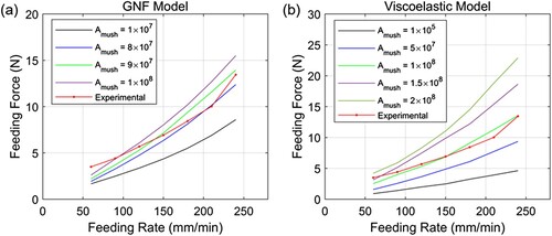
Moreover, we computed the average deviation to assess the precision of predicting the steady-state feeding force. The GNF model showed a deviation of 14.6%, while the viscoelastic model exhibited approximately 8.9%. The viscoelastic model demonstrates superior prediction accuracy compared to the GNF model. Consequently, the viscoelastic model could be a substantial enhancement in predicting the steady-state feeding force for semi-crystalline polymers (e.g. PLA) in FDM compared to relevant research [9]. In addition, our research in feeding force prediction has met or surpassed the predictive levels seen in studies on amorphous polymers like ABS (Acrylonitrile Butadiene Styrene), PS (Polystyrene), and PC (Polycarbonate) in FDM process [3,6,8,47].

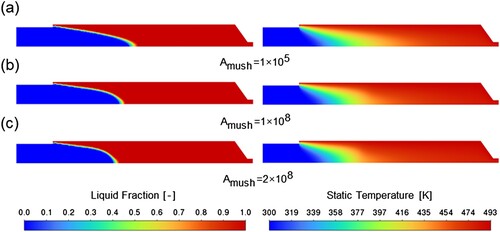
Furthermore, as shown in Figure 3, with a smaller $A_{\mathrm{mush}}$ and under the same feeding rate, the solid–liquid interface becomes closer to the outlet. Interestingly, the proportion of the solid phase does not visibly increase with the rise of $A_{\mathrm{mush}}$. This can potentially be explained by considering the distribution of the liquid phase. As $A_{\mathrm{mush}}$ increases, the solid phase region tends to expand towards the wall. On the basis of the temperature distribution (Figure 4), it becomes apparent that a substantial gradient in temperature exists near the wall in comparison to the central zone. Also, the flow rate exhibits its peak magnitude at the central axis, gradually diminishing to zero in proximity to the wall. This illustrates an increase in viscosity as the fluid approaches the wall due to the shear thinning of non-Newtonian fluids. Thus, the increase in viscosity caused by the temperature drop near the wall becomes more pounced. Conversely, in the central zone, the viscosity increases due to the temperature drop is significantly mitigated by the larger shear rate and notable shear thinning effect. Therefore, as $A_{\mathrm{mush}}$ becomes larger, the feeding force continues to rise despite the limited or even decreased proportion of the solid phase.

Figure 4. Influence of different $A_{\mathrm{mush}}$ on the simulation results for the liquid phase fraction and temperature distribution at different $A_{\mathrm{mush}}$.

3.2. Response of the feeding force

This section focuses on investigating the transient changes of the feeding force exerted on the filament during the feeding process, considering the viscoelasticity of the material. The significance of the research lies in the fact the successful extrusion of the filament in the FDM process requires overcoming the varying transient feeding force caused by the complex melt flow in the hot-end. This implies that the motor’s performance (e.g. power, torque, rotational velocity) should be adapted to accommodate these transient feeding force variations. The simulation begins from a pause in printing, without considering retraction. In other words, the liquefier is filled with polymer melt prior to feeding, and the filament’s speed is varied from zero.

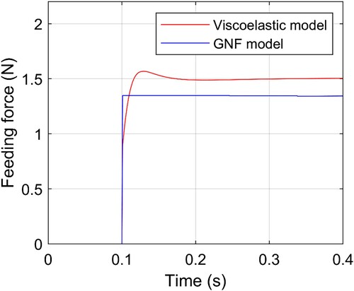
Under the isothermal flow assumption, this section analyses and compares the response of the feeding force under two models: the GNF model, which considers only the viscous effect, and the Giesekus model, which incorporates the complete viscoelasticity of polymers. The viscosity and other parameters for both models are fitted at a reference temperature (453.15 K). A step signal is applied to the velocity at the flow field inlet, set at 60 mm/min. The results (Figure 5) demonstrated that the introduction of the viscoelastic model leads to higher predicted feeding forces compared to that of the purely viscous model, which neglects the elastic effect. Moreover, due to its ability to capture polymer elasticity, the viscoelastic model exhibits a greater accuracy in capturing transient changes of feeding force for a small overshoot during the rising stage of extrusion. While this overshoot has been observed in both numerical simulations and experiments involving simple pipeline flow or simple shear flow in viscoelastic fluids [48–53], such as $C_{100}{H}_{202}$ and blood. If the overshoot becomes apparent, it indicates that the motor for the feeding filament should be adjusted accordingly to precisely regulate the extrusion flow rate. Additionally, the moving speed of the extruder can be also adjusted to mitigate the strand width variation. This overshoot is attributed to the elastic accumulation and relaxation of the polymer melt. The relaxation time of the polymer represents the time lag in the development of the stress, following the imposition of the shear rate. Although the polymer generally has multiple relaxation times or even a continuous relaxation time spectrum, it can be simply estimated with the one-mode Maxwell model [54–56]. The overall time lag can be understood as the ratio of the storage modulus to the loss modulus, which is the inverse of the damping ratio [56–58]. This implies that polymers with high damping exhibit less pronounced overshoot phenomenon during the FDM process, such as thermoplastic polyurethane (TPU) [59], while those with low damping show more obvious hysteresis and overshoot, affecting the printing quality.

Figure 5. Prediction of transient feeding force under the isothermal flow assumption.

During actual printing, the flow of the polymer in the hot-end is inevitably non-isothermal. This non-isothermal flow introduces a more complex relationship between the feeding force and feeding rate. In this study, the GNF model and the viscoelastic model are used for predicting and comparing the response of feeding force under different input velocity curves. Two types of velocity profiles are selected as input: a step signal (Figure 6 (a)) and a trapezoidal signal (Figure 6 (b)) that is closer to the actual FDM extrusion process. The target feeding rates are 80 and 240 mm/min, respectively. However, the experimental instrument used in our study has a maximum frequency of 1 Hz, under which it is difficult to capture the complete variation of transient forces. To validate and assess the computational model, the computational results are compared to the existing experimental research [3,7,60].

Figure 6. Feeding force response with the GNF model (c) and viscoelastic model (e) under the step velocity input (a). Feeding force response with the GNF model (d) and viscoelastic model (f) under the trapezoidal velocity profile (b).

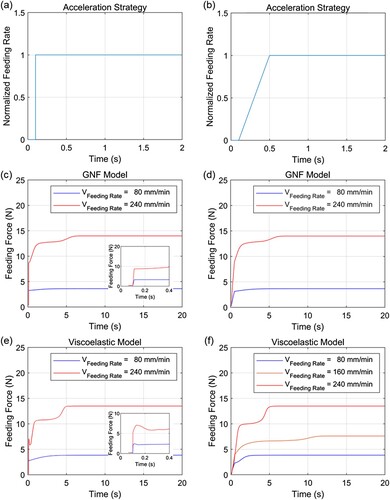
The simulation results show that for the step velocity input, when the inlet velocity changes, it is found that there is an instantaneous step rise of feeding force in the GNF model (Figure 6 (c)). Conversely, the viscoelastic model exhibits a transient overshoot oscillation of the feeding force (Figure 6 (e)), which becomes more pronounced with higher feeding rates. Meanwhile, for the trapezoidal velocity input, the GNF model predicts the feeding force that is more linear during the acceleration stage (Figure 6 (d)). In addition, the feeding force prediction curves of the two constitutive models have a similar feature, that is, at a high feeding rate (240 mm/min) (Figure 6 (c–f)) the simulated feeding force shows a sudden increase in feeding force after a steady acceleration. This occurrence happens when the low-temperature PLA filament (i.e. the new entry filament) enters the liquefier. The filament melts, replacing the pre-existing high-temperature PLA in the hot-end. The temperature distribution inside the liquefier stabilises before the new entry filament approaches the conical section, so the feeding force does not change. However, when feeding at high speed, there is a double increase for filament passing through the channel. The corresponding explanations are made as follows:

It is known in Section 3.1 that the increase in viscosity due to temperature drop is much greater near the wall than near the centre of the channel. Therefore, before the new entry filament passes through the conical section, although the temperature drop zone at the centre expands, the area of the temperature drop zone near the wall does not change significantly. So the ascent of the feeding force gradually slows down. However, when the new entry filament passes through the conical section (Zone II) and the outlet section (Zone III) in Figure 1, the diameter of the flow channel decreases and the temperature of the wall near the conical section and the exit section drops distinctly. Consequently, the feeding force rises further at the corresponding time point. Moreover, this rise is more prominent as the feeding rate increases (Figure 6 (f)), as validated by the experiments in [60].

Furthermore, it is observed that the GNF model predicts less significant feeding forces during this stage when compared to the viscoelastic model (Figure 6 (c–f)). However, the study by Serdeczny et al. [47] revealed that a second increase in feeding force is more noticeable at high feeding rates, followed by fluctuations due to the unstable fill level of the gap. This phenomenon will be taken into account in future studies by changing the free-slip wall (Figure 6) and coupling the multiphase model [3,7].

3.3. Viscoelastic behaviour in extrusion

This section focuses on the viscoelastic phenomena of polymer in the steady-state extrusion process of FDM and analyses the mechanism of polymer interaction in the flow channel. The changes in viscosity and elasticity at different feeding rates are understood, and an appropriate method is proposed to measure the influence of viscoelasticity on the FDM printing process.

3.3.1. Viscoelastic dynamics

The relationship between the stress field, flow field, and phase transition process is directly linked to the influence of stress terms ($\mathrm{\nabla }\cdot \mathit{\tau }$, $\stackrel{=}{\mathit{\tau }}:\mathrm{\nabla }\mathit{u}$) in the governing equations (Equation (1)–(3)). Thus, the distribution of the stress field is influenced mutually by the evolution of the polymer’s temperature and velocity fields in the hot-end, and it affects the formation of extruded polymer strands during the deposition process [61]. Hence, examining the local distribution of stress in the flow channel is of great significance in comprehending the melting flow mechanism of the polymer in the hot-end.

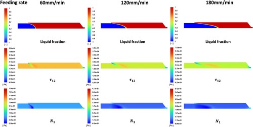
The simulation is based on a simplified 2D model, the stress tensor is a 2 × 2 symmetric matrix with four components, ${\tau }_{11}$, ${\tau }_{12}$, ${\tau }_{21}$, and ${\tau }_{22}$, of which ${\tau }_{12}={\tau }_{21}$, is the shear stress, which is related to the viscous action of the polymer. While the other two components, axial stress ${\tau }_{11}$ and radial stress ${\tau }_{22}$, are mainly related to the elasticity of the polymer. Taking the simulation results at a feeding rate of 60 mm/min as an example, the characteristics and causes of the stress distribution in the hot-end (Figure 7) are analysed in two parts, one is from the inlet of the runner to before the tapered convergence section (Zone I in Figure 7) and the other is from the tapered convergence section of the runner to the outlet section (Zones II and III in Figure 7).

Figure 7. Distribution for solid-liquid phase, streamline and each component of the stress tensor at a feeding rate of 60 mm/min.

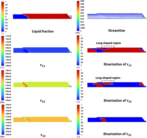
Between the conical convergence section and the outlet (Zones II and III), as shown in Figure 7, the diameter reduction results in the conservation of flow rate, leading to a sharp increase in flow velocity, which results in sharp changes in the various stress components. Near the wall of the conical convergence section (Zone II), ${\tau }_{11}$ and ${\tau }_{22}$ undergo a change from positive to negative or negative to positive. The possible reasons for this change are as follows:

• For the axial component of the stress tensor ${\tau }_{11}$, the fluid undergoes compression at the conical wall, experiences a turn, and the corresponding axial velocity is reduced, leading to negative axial stress ${\tau }_{11}$.

• For the radial component of the stress tensor ${\tau }_{22}$, the fluid near the wall enters the conical section and experiences a turn, producing higher radial downward velocity. The radial velocity gradually decreases in the process of flowing towards the centre resulting in a positive velocity gradient and radial stress ${\tau }_{22}$ near the wall, hence, the fluid near the wall is under tension. The fluid near the centre is squeezed, and the velocity gradient and radial stress ${\tau }_{22}$ are negative.

Before the entrance to the conical convergence section, the stress distribution is mainly gathered near the phase-change interface, and the various stress components show different degrees of stress concentration near the phase-change interface (Figure 7). It reveals that the elasticity has an important effect on the phase transformation of semi-crystalline polymers. For instance, the axial component ${\tau }_{11}$ takes a negative value near the phase transition interface in the solid domain where the diameter of the filament is smaller than that of the flow channel. As illustrated by the streamline in Figure 7, the polymer filament will naturally diffuse toward the wall during the melting process, and this diffusion phenomenon results in the solid under the phase interface being pulled, i.e. the radial component ${\tau }_{11}$ is positive. Due to mass conservation, the velocity of the filament feed is necessarily greater than the average velocity of the fluid in the flow channel in the liquefier Zone I. This causes the solid filament to be compressed near the phase-change interface. In addition, a lung-shaped positive and negative boundary region appears above the phase change interface in the stress binarization of ${\tau }_{11}$ and ${\tau }_{22}$ in Figure 7, which is not observed in the stress distribution diagram. This disparity arises from the inability to achieve an instantaneous change in fluid velocity as the PLA filament transitions from the solid to the liquid phase. Moreover, the solid filaments that do not enter the fluid section at the inlet exhibit a notable concentration of stresses in proximity to the reflux point. The recirculation region towards the inlet obviously brings upward frictional forces on the filaments, making the axial component ${\tau }_{11}$ negatives While this happens at the boundary point of the phase-change interface, the filaments undergo melt diffusion making the radial component ${\tau }_{22}$ positive.

3.3.2. Viscoelastic effects on the FDM printing process

To study the effect of viscoelasticity on the printing process, the stresses in the filament during printing are calculated from the numerical model. Firstly, the shear stress ${\tau }_{12}$ is used to characterise the viscous effect. Then the normal stress difference $N_1$ (i.e. $N_1={\tau }_{11}-{\tau }_{22}$) is introduced as the indicator of elasticity, which is only related to the polymer elasticity and is zero in the generalised Newtonian fluid (GNF) mechanics model [62,63] (Figure 8). It is found that the stress concentration near the phase change interface weakens during the process of increasing velocity (Figure 8). This is because the gap between the filament velocity and the average fluid velocity is becoming smaller in proportion to the overall velocity, and the diffusion phenomenon becomes less and less evident.

Figure 8. Comparison of distribution for normal stress difference $N_1$ and shear stress ${\tau }_{12}$ at different feeding rates.

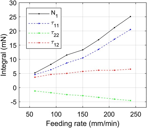
Furthermore, the effect of the viscoelastic effect on the FDM printing process is also investigated by analysing the stress changes at the nozzle outlet. At the outlet (with zero relative pressure), the components of the stress tensor and the normal stress difference $N_1$ are integrated over the area of the outlet, and these stress integral curves are plotted against feeding rates in Figure 9. It is found that, as the feeding rate increases, the increase in the normal stress difference integral at the outlet is much more significant than the increase in the shear stress integral. It reveals that the effect of polymer elasticity on the printing process dominates as the feeding rate increases. Additionally, the stress tensor $\mathit{\tau }$ at the outlet can serve as the initial condition for the simulation study of the FDM deposition process. This provides a more realistic simulation and prediction of the distribution of residual stresses in the printed parts during the FDM process. Therefore, it can be used for better optimising the process parameters and the design of the hot-end.

Figure 9. Curves about the area integral at the outlet for the normal stress difference and each stress tensor component versus the feeding rate.

4. Conclusion

This paper presents a viscoelastic constitutive model to investigate the transient and steady-state melting flow and viscoelastic behaviour of polymer filaments in the hot-end of an FDM printer. The model utilises the enthalpy-porosity method to describe the phase transition process of semi-crystalline polymers, i.e. polylactic acid, which exhibits a notable phase transition process. The parameters for the constitutive model and the time-temperature equivalence principle are determined through rheological experiments. The influence of the empirical parameter $A_{\mathrm{mush}}$ on the feeding force is studied. Also, its optimal value is experimentally identified. The following conclusions and prospects can be drawn:

• The empirical parameter $A_{\mathrm{mush}}$ values in the enthalpy-porosity model describing the phase transition has a distinct influence on the simulation results, including feeding force and temperature distribution. Increasing the mushy zone parameter $A_{\mathrm{mush}}$ leads to a gradual rise in the feeding force and a slower molten process of the filament. By optimising this parameter, the viscoelastic model will have a better agreement with experimental measurements.

• The viscoelastic constitutive model captures the transient behaviour of the FDM feeding force, including the overshoot and lag phenomenon caused by the elastic effect of polymer, which cannot be modelled by the generalised Newtonian model. However, this phenomenon is not fully validated in this study due to the limitation of current measurement setup. Meanwhile, our model has limitations in simulating the dynamic filling process of the gap between the filament and the channel wall. This hampers its ability to accurately predict feeding force at high feeding rates. Therefore, further refinement involves incorporating gas–liquid multi-phase flow into the numerical model and improving the measurement of transient feeding force.

• During steady-state feeding, the viscoelastic effect becomes more prominent relative to the viscous effect as the feeding speed increases. This results in a larger residual stress in the extruded filament. Studying the viscoelastic behaviour in extrusion flow enables the generation of an initial stress distribution for FDM deposition simulation, facilitating accurate and comprehensive prediction of strand formation and residual-stress distribution in printed parts. Understanding these viscoelastic effects quantitatively is crucial for optimising process parameters and hot-end design.

Acknowledgement

We would also like to express our gratitude to INTAMSYS Technology Co., LTD. for generously providing the experimental data on steady feeding force at various speeds.

Disclosure statement

No potential conflict of interest was reported by the author(s).

Data availability statement

The data that support the findings of this study are available from the corresponding author, [YX], upon reasonable request.

Correction Statement

This article has been corrected with minor changes. These changes do not impact the academic content of the article.

Additional information

Funding

This work was supported by National Natural Science Foundation of China: [Grant Number grant number 52105261]; Guangdong Innovative and Entrepreneurial Research Team Program: [Grant Number 2021ZT09X256]; Shenzhen Science and Technology Innovation Committee: [Grant Number JCYJ20210324104610028].

Appendix

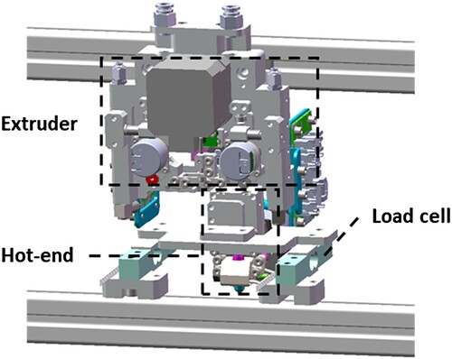
The experiment setup is based on a modified INTAMSYS PRO410 3D printer (INTAMSYS Technology Co., LTD). The setup is divided into two parts: an upper part for the extruder, fixed by a metal frame, and a lower part for the hot-end, solely attached to a load cell (GML611-5 kg, GALOCE (XI'AN) M&C Technology Co., LTD.). The load cell is secured to the metal frame, as depicted in Figure A1. In other words, the load cell is mounted between the extruder and the hot-end and is used to measure the feeding force.

Figure A1. Experiment setup of feeding force measurement instrument.

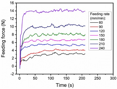
The equipment has a maximum measurement frequency of 1 Hz. Prior to testing, a pre-extrusion process is conducted to ensure that the polymer filament fills the flow channel of the hot-end at zero feeding rate. The testing begins with applying a trapezoidal acceleration signal to accelerate to the target feeding rate. The total testing time is 200 s. The feeding force at a given feeding rate is calculated as the average of data measured during 100- 200 s (Figure A2).

Figure A2. Experimental data curves of feeding force at different feeding rates.

References

- Hull CW. (1986). “Apparatus and method for creating three-dimensional objects.” Google Patents. https://patents.google.com/patent/US5121329A/en.
- Cano-Vicent A, Tambuwala MM, Hassan SS, et al. Fused deposition modelling: current status, methodology, applications and future prospects. Add Manuf. 2021;47(November):102378, doi:10.1016/J.ADDMA.2021.102378
- Marion S, Sardo L, Joffre T, et al. First steps of the melting of an amorphous polymer through a hot-end of a material extrusion additive manufacturing. Add Manuf. 2023;65(March):103435, doi:10.1016/J.ADDMA.2023.103435
- Nzebuka GC, Ufodike CO, Rahman AM, et al. Numerical modeling of the effect of nozzle diameter and heat flux on the polymer flow in fused filament fabrication. J Manuf Process. 2022;82(October):585–600. doi:10.1016/j.jmapro.2022.08.029
- Pigeonneau F, Xu D, Vincent M, et al. Heating and flow computations of an amorphous polymer in the liquefier of a material extrusion 3D printer. Add Manuf. 2020;32(August 2019). doi:10.1016/j.addma.2019.101001
- Ufodike CO, Nzebuka GC. Investigation of thermal evolution and fluid flow in the hot-end of a material extrusion 3D printer using melting model. Add Manuf. 2022;49(January). doi:10.1016/j.addma.2021.102502
- Serdeczny MP, Comminal R, Mollah MT, et al. Numerical modeling of the polymer flow through the hot-end in filament-based material extrusion additive manufacturing. Add Manuf. 2020;36(December). doi:10.1016/j.addma.2020.101454
- Kattinger J, Ebinger T, Kurz R, et al. Numerical simulation of the complex flow during material extrusion in fused filament fabrication. Add Manuf. 2022;49(January) doi:10.1016/j.addma.2021.102476..
- Phan DD, Horner JS, Swain ZR, et al. Computational fluid dynamics simulation of the melting process in the fused filament fabrication additive manufacturing technique. Add Manuf. 2020;33(May). doi:10.1016/j.addma.2020.101161
- Xu X, Ren H, Chen S, et al. Review on melt flow simulations for thermoplastics and their fiber reinforced composites in fused deposition modeling. J Manuf Process. 2023;92(April):272–286. doi:10.1016/J.JMAPRO.2023.02.039
- Ren H, Yang X, Wang Z, et al. Smart structures with embedded flexible sensors fabricated by fused deposition modeling-based multimaterial 3D printing. Int J Smart Nano Mater. 2022;13(3):447–464. doi:10.1080/19475411.2022.2095454
- Go J, Schiffres SN, Stevens AG, et al. Rate limits of additive manufacturing by fused filament fabrication and guidelines for high-throughput system design. Add Manuf. 2017;16(August):1–11. doi:10.1016/j.addma.2017.03.007
- Peng F, Vogt BD, Cakmak M. Complex flow and temperature history during melt extrusion in material extrusion additive manufacturing. Add Manuf. 2018;22(May):197–206. doi:10.1016/j.addma.2018.05.015
- Shaqour B, Abuabiah M, Abdel-Fattah S, et al. Gaining a better understanding of the extrusion process in fused filament fabrication 3D printing: a review. Int J Adv Manuf Technol. 2021;114(5–6):1279–1291. doi:10.1007/s00170-021-06918-6
- Pricci A, Al Islam Ovy SM, Stano G, et al. Semi-analytical and numerical models to predict the extrusion force for silicone additive manufacturing, as a function of the process parameters. Add Manuf Lett. 2023;6(May). doi:10.1016/j.addlet.2023.100147
- Hart KR, Dunn RM, Sietins JM, et al. Increased fracture toughness of additively manufactured amorphous thermoplastics via thermal annealing. Polymer. 2018;144:192–204. doi:10.1016/j.polymer.2018.04.024
- Yang F, Pitchumani R. Healing of thermoplastic polymers at an interface under nonisothermal conditions. Macromolecules. 2002;35(8):3213–3224. doi:10.1021/ma010858o
- McIlroy C, Olmsted PD. Disentanglement effects on welding behaviour of polymer melts during the fused-filament-fabrication method for additive manufacturing. Polymer. 2017;123:376–391. doi:10.1016/j.polymer.2017.06.051
- Serdeczny MP, Comminal R, Mollah MT, et al. Viscoelastic simulation and optimisation of the polymer flow through the hot-end during filament-based material extrusion additive manufacturing. Virtual Phys Prototyp. 2022;17(2):205–219. doi:10.1080/17452759.2022.2028522
- Christensen R. Theory of viscoelasticity. New York (NY): Elsevier; 1982.
- Comminal R, Pimenta F, Hattel JH, et al. Numerical simulation of the planar extrudate swell of pseudoplastic and viscoelastic fluids with the streamfunction and the VOF methods. J Non-Newtonian Fluid Mech. 2018;252(December 2017):1–18. doi:10.1016/j.jnnfm.2017.12.005
- Tang D, Marchesini FH, Cardon L, et al. Three-dimensional flow simulations for polymer extrudate swell out of slit dies from low to high aspect ratios. Phys Fluids. 2019;31(9). doi:10.1063/1.5116850
- Cao W, Shen Y, Wang P, et al. Viscoelastic modeling and simulation for polymer melt flow in injection/compression molding. J Non-Newtonian Fluid Mech. 2019;274(December):104186, doi:10.1016/J.JNNFM.2019.104186
- Rothstein JP, McKinley GH. Extensional flow of a polystyrene Boger fluid through a 4 : 1 : 4 axisymmetric contraction/expansion. J Non-Newtonian Fluid Mech. 1999;86(1–2):61–88. doi:10.1016/S0377-0257(98)00202-X
- Kwon I, Chun MS, Jung HW, et al. Determination of draw resonance onsets in tension-controlled viscoelastic spinning process using transient frequency response method. J Non-Newtonian Fluid Mech. 2016;228(February):31–37. doi:10.1016/J.JNNFM.2015.12.006
- Lee JS, Shin DM, Song HS, et al. Existence of optimal cooling conditions in the film blowing process. J Non-Newtonian Fluid Mech. 2006;137(1–3):24–30. doi:10.1016/J.JNNFM.2005.12.011
- Schuller T, Fanzio P, Galindo-Rosales FJ. Analysis of the importance of shear-induced elastic stresses in material extrusion. Add Manuf. 2022: 102952, doi:10.1016/J.ADDMA.2022.102952
- Giesekus H. A simple constitutive equation for polymer fluids based on the concept of deformation-dependent tensorial mobility. J Non-Newtonian Fluid Mech. 1982;11(1–2):69–109. doi:10.1016/0377-0257(82)85016-7
- Hong Y, Mrinal M, Phan HS, et al. In-Situ observation of the extrusion processes of acrylonitrile butadiene styrene and polylactic acid for material extrusion additive manufacturing. Add Manuf. 2022;49(January). doi:10.1016/j.addma.2021.102507
- Bird RB, Curtiss CF, Armstrong RC, et al. Dynamics of polymer liquids. journal of polymer science part C: polymer letters. New York (NY): John Wiley & Sons; 1987.
- Bennon WD, Incropera FP. A continuum model for momentum: heat and species transport in binary solid-liquid phase change systems – I. Model formulation. Int J Heat Mass Transfer. 1987;30(10):2161–2170. doi:10.1016/0017-9310(87)90094-9
- Arrhenius S. Über Die Reaktionsgeschwindigkeit Bei Der Inversion von Rohrzucker Durch Säuren. Z Phys Chem. 1889;4(1):226–248. doi:10.1515/ZPCH-1889-0416
- Polymaker. (2019). “PolyLiteTM PLA.” https://us.polymaker.com/products/polylite-pla%0Ahttps://polymaker.com/product/polylite-pla/.
- Voller VR, Prakash C. A fixed grid numerical modelling methodology for convection-diffusion mushy region phase-change problems. Int J Heat Mass Transfer. 1987;30(8):1709–1719. doi:10.1016/0017-9310(87)90317-6
- Marri GK, Balaji C. Liquid crystal thermography based study on melting dynamics and the effect of mushy zone constant in numerical modeling of melting of a phase change material. Int J Therm Sci. 2022;171(June 2021):107176, doi:10.1016/j.ijthermalsci.2021.107176
- Parry AJ, Eames PC, Agyenim FB, et al. “Modeling of thermal energy storage shell-and- tube heat exchanger modeling of thermal energy storage shell-and-tube heat exchanger. Heat Transfer Eng. 2014: 7632, doi:10.1080/01457632.2013.810057
- Tutar M, Karakus A. 3-D computational modelling of process condition effects on polymer injection molding. Int Polym Process. 2009;24(5):384–398. doi:10.3139/217.2249
- Jung UH, Kim JH, Kim JH, et al. Numerical investigation on the melting of circular finned PCM system using CFD & full factorial design. J Mech Sci Technol. 2016;30(6):2813–2826. doi:10.1007/s12206-016-0541-7
- Fadl M, Eames PC. Numerical investigation of the influence of mushy zone parameter amush on heat transfer characteristics in vertically and horizontally oriented thermal energy storage systems. Appl Therm Eng. 2019;151(June 2018):90–99. doi:10.1016/j.applthermaleng.2019.01.102
- Nzebuka GC, Waheed MA. Thermal evolution in the direct chill casting of an Al-4 Pct Cu alloy using the low-reynolds number turbulence model. Int J Therm Sci. 2020;147(January):106152, doi:10.1016/J.IJTHERMALSCI.2019.106152
- Kaviany M. Principles of heat transfer in porous media, Mechanical Engineering Series. New York (NY): Springer US; 1991.
- Xu P, Yu B. Developing a New form of permeability and Kozeny–Carman constant for homogeneous porous media by means of fractal geometry. Adv Water Res. 2008;31(1):74–81. doi:10.1016/J.ADVWATRES.2007.06.003
- Nzebuka GC, Ufodike CO, Egole CP. Influence of various aspects of low-reynolds number turbulence models on predicting flow characteristics and transport variables in a horizontal direct-chill casting. Int J Heat Mass Transfer. 2021;179(November):121648, doi:10.1016/J.IJHEATMASSTRANSFER.2021.121648
- Waheed MA, Nzebuka GC. Analysis of thermally driven flow pattern formation in aluminium DC casting for different Rayleigh numbers and billet diameters. Therm Sci Eng Progr. 2020;18(August):100536, doi:10.1016/J.TSEP.2020.100536
- Zalba B, Marín JM, Cabeza LF, et al. Review on thermal energy storage with phase change: materials, heat transfer analysis and applications. Appl Therm Eng. 2003;23(3):251–283. doi:10.1016/S1359-4311(02)00192-8
- Ziskind G. Modeling of heat transfer in phase change materials for thermal energy storage systems. In: Luisa F. Cabeza, editor. Advances in thermal energy storage systems. Duxford: Methods and Applications. LTD; 2020. p. 359–379.
- Serdeczny MP, Comminal R, Pedersen DB, et al. Experimental and analytical study of the polymer melt flow through the hot-end in material extrusion additive manufacturing. Add Manuf. 2020;32(December 2019):100997, doi:10.1016/j.addma.2019.100997
- Varchanis S, Tsamopoulos J, Shen AQ, et al. Reduced and increased flow resistance in shear-dominated flows of oldroyd-B fluids. J Non-Newtonian Fluid Mech. 2022;300(February):104698, doi:10.1016/J.JNNFM.2021.104698
- Ghigo AR, Lagrée PY, Fullana JM. A time-dependent non-newtonian extension of a 1D blood flow model. J Non-Newtonian Fluid Mech. 2018;253(March):36–49. doi:10.1016/J.JNNFM.2018.01.004
- Keshtiban IJ, Puangkird B, Tamaddon-Jahromi H, et al. Generalised approach for transient computation of start-up pressure-driven viscoelastic flow. J Non-Newtonian Fluid Mech. 2008;151(1–3):2–20. doi:10.1016/J.JNNFM.2008.03.004
- Ellero M, Tanner RI. SPH simulations of transient viscoelastic flows at Low reynolds number. J Non-Newtonian Fluid Mech. 2005;132(1–3):61–72. doi:10.1016/J.JNNFM.2005.08.012
- Oliveira PJ. Reduced-Stress method for efficient computation of time-dependent viscoelastic flow with stress equations of FENE-P type. J Non-Newtonian Fluid Mech. 2017;248(October):74–91. doi:10.1016/J.JNNFM.2017.09.001
- Moore JD, Cui ST, Cochran HD, et al. A molecular dynamics study of a short-chain polyethylene melt: II. Transient response upon onset of shear. J Non-Newtonian Fluid Mech. 2000;93(1):101–116. doi:10.1016/S0377-0257(00)00104-X
- Tran E, Clarke A. The relaxation time of entangled HPAM solutions in flow. J Non-Newtonian Fluid Mech. 2023;311(August 2022):104954, doi:10.1016/j.jnnfm.2022.104954
- Baumgaertel M, Winter HH. Interrelation between continuous and discrete relaxation time spectra. J Non-Newtonian Fluid Mech. 1992;44(September):15–36. doi:10.1016/0377-0257(92)80043-W
- Swallowe GM. Relaxations in polymers. Mech Prop Test Polym: An A–Z Ref. 1999: 195–198. doi:10.1007/978-94-015-9231-4_42
- Huilgol RR, Phan-Thien N, ed. Constitutive equations derived from microstructures. In: Rheology series. Amsterdam: Elsevier; 1997;6:155–270.
- Kiparissides C, Pladis P, Moen Ø. From polyethylene rheology curves to molecular weight distributions. Comput Aided Chem Eng. 2006;22(C):241–255. doi:10.1016/S1570-7946(06)80013-1
- Hofmann J, Maier U, Prage FH, Vogel J. Determination of the Composition and Properties of Polyurethanes. In: Günter Oertel and L. (Lothar) Abele, editors. Polyurethane Handbook : Chemistry, Raw Materials, Processing, Application, Properties, New York (NY): Hanser, 1994; 45:479–549.
- Moretti M, Rossi A, Senin N. In-Process simulation of the extrusion to support optimisation and real-time monitoring in fused filament fabrication. Add Manuf. 2021;38(October 2020):101817, doi:10.1016/j.addma.2020.101817
- Xia H, Lu J, Tryggvason G. A numerical study of the effect of viscoelastic stresses in fused filament fabrication. Comput Methods Appl Mech Eng. 2019;346(April):242–259. doi:10.1016/j.cma.2018.11.031
- Mieras HJMA, Van Rijn CFH. Elastic behaviour of some polymer melts. Nature. 1968;218(5144):865–866. doi:10.1038/218865b0
- James DF. N1 stresses in extensional flows. J Non-Newtonian Fluid Mech. 2016;232(June):33–42. doi:10.1016/j.jnnfm.2016.01.012