Integrated vehicle chassis fabricated by wire and arc additive manufacturing: structure generation, printing radian optimisation, and performance prediction

ABSTRACT

In the automotive industry, the extended design and iteration cycles for integrated chassis typically span 2–3 years, creating a misalignment with swiftly changing market demands. Wire arc additive manufacturing (WAAM) technology presents a viable alternative, overcoming the limitations of conventional chassis production. Our holistic framework significantly condenses the design, optimisation, and validation stages for automotive chassis. Initially, a ground structure method is utilised to outline and generate a skeleton chassis. We then utilise the OpenCV image processing method to select a hollow skeleton chassis with minimal material occupancy (0.476) and suspension printing. Subsequently, we assess the influence of printing radian variations by the robotic arm on the microstructure and stress, employing a cellular automaton-finite element (CA-FE) model at the 150th and 200th layer benchmarks. A Kalman filter (KF) is also implemented to fine-tune the printing radian in regions with coarse grain structures and elevated solute concentrations. The process concludes with collision and modal simulation verifications of the skeleton chassis, affirming the optimisation's success. This streamlined methodology allows the completion of the chassis design and manufacturing cycle within a remarkably condensed time frame of one week, accelerating the development process by a factor of 120.

KEYWORDS:

• WAAM
• FEM
• cellular automata
• topology
• Kalman filtering

1. Introduction

Under the trend of new energy vehicles, the integration of medium and large-scale structural manufacturing of commercial vehicles is becoming the main focus of development. This involves accelerating the performance improvement of various vehicle components and reducing the research and development cycle. Nevertheless, achieving structural lightweight and performance optimisation in traditional gauge-level chassis is a time-consuming process, which has gained significant attention from both the industry and businesses.

The topological structure design based on wire arc additive manufacturing (WAAM) can achieve high value-added components [1] and complex geometric shapes that are difficult to achieve by traditional milling or casting processes. This is done by constructing components layer by layer, which has the potential to shorten the development cycle of vehicle-level chassis.

The topological structure and mechanical properties of low-speed commercial electric vehicles pose challenges in terms of printing large structural parts. To address these issues, scholars have employed innovative design methods such as topology optimisation, cell structure, and mixed materials to determine material distribution. This has led to advancements in the field of Additive Manufacturing Design (DFAM) [2,3], including continuum [4] and discrete ground structure [5] topology optimisation methods. Wang et al. [6] proposed the Constructed Solid Geometry (CSG) method, which utilises genetic algorithms to select the optimal design from multiple variants. For geometric microstructure problems, Wang et al. [7] developed a method to describe the yarn structure in 3D braided preforms. In the context of large-scale structural optimisation, Wu et al. [8] introduced the moving asymptote (MMA) method for porous structure filling design, simplifying the description of geometric structures of hollow tubes. Bai, Zuo, Guo, et al. [9,10] utilised the moving deformable member model (MMC), a continuum optimisation model, to design the hollow frame of a vehicle. Zhang, Yu, Xu, et al. [11] proposed a tubular topological honeycomb structure with structural hierarchy and verified its mechanical reliability. However, the aforementioned structural explorations do not consider the evolution of material microstructure within the geometric structure. Therefore, alternative methods can be employed to further investigate the microstructure.

As a widely used meso-micro simulation method in the field of metal additive manufacturing (MAM), cellular automaton and finite element (CA-FE) differs from the typical thermodynamic simulation used in macro-scale computational domains [12]. In the domain of microstructure simulation, it is necessary to limit the volume to a small size [13] because the grain structure and texture are primarily determined at high temperatures and are no longer influenced by the heat source moving further away. However, the region should still be large enough to allow for a re-melting effect through continuous layer accumulation. Researchers in the field of MAM have employed various microstructure simulation methods, including phase field [14], Monte Carlo [15], cellular automata (CA) simulation [16], as well as empirical modelling [17]. Among these methods, cellular automata technology can simultaneously consider both deterministic and probabilistic solidification phenomena. Originally developed by Rappaz [18] and Gandin [19] to simulate grain structure during casting solidification, this technique allows for an easy explanation of the competition between microstructure mechanisms through the effective calibration of parameters. To calculate the thermal field and temperature gradient, this method needs to be combined with thermal simulation. Various thermal analysis methods, such as finite element [20], finite volume [21], and finite difference (FD) [22], have been coupled with cellular automata in the existing literature. However, a single mesoscopic simulation is insufficient to optimise the printing trajectory in additive manufacturing, as it only explores the formation laws of microstructure.

In the field of additive manufacturing printing trajectories, Kaji [23] and Guidetti [24] proposed a technique that utilises a non-parallel slicing method for constructing complex components, such as curved pipes, to achieve non-parallel deposition. Huang et al. [25] also developed a self-developed post-processing algorithm that converts the determined path into a continuous carbon fibre printing tool path with reduced overlap, aiming to reduce material usage. Furthermore, Jin et al. [26] utilise the inclination angle of the printing reference line to generate sub-path segments of the tool and connect these sub-paths as needed to enhance printing efficiency and accuracy.

Research into the accelerated design, iterative optimisation, and validation of integrated automotive chassis topologies through wire arc additive manufacturing (WAAM) remains scarce. In our investigation, we applied the ground structure method to generate an ensemble of 44 unique three-dimensional hollow chassis skeletons. OpenCV, an advanced image processing technology, was harnessed to ascertain the material and suspension printing distributions for these chassis structures with a dimensionality reduction approach. We further implemented the CA-FE method to probe the microstructural and stress distributions within the robotic arm across varying topological configurations, encompassing 150 and 200-layer constructs. Our analysis of the stress state draws upon data derived from residual stress testing and microstructure simulation imagery. In contrast to the digital image correlation (DIC) surface curvature measurement translated into in-plane residual stress estimations [27], our methodology facilitates swift detection of stress singularities, thereby markedly enhancing the throughput of regional residual stress measurements. Moreover, the Kalman filter (FV) method was employed to refine the printing layer by filtering out coarse crystal regions and areas of high solute concentration. This refinement enables the fine-tuning of the robotic arm’s printing arc without necessitating alterations to the printing trajectory. For the optimised skeleton chassis, we conducted collision and modal analysis to verify the vibration performance reliability of the hub area and the overall chassis structure near the printing layers 150 and 200. Our proposed method eliminates the need for a large amount of difficult-to-determine experimental data and shortens the chassis iteration cycle to one week, making it suitable for any metal 3D printing scheme.

2. Materials and methods

In this experiment and production, we selected 7075 aluminum alloy welding wire with a diameter of 1.2 mm as the deposition material. The substrate material used was a 7075 aluminum alloy rolling plate in the T6 state. The chemical composition of both the welding wire and the substrate can be found in Table 1. Prior to arc deposition, the substrate underwent grinding using a grinding machine to remove the surface oxide skin. It was then cleaned with acetone to remove any organic matter. After drying, the substrate was preheated to 80°C using the flame method and prepared for deposition.

Table 1. Main chemical compositions of 7075 aluminum alloy welding wires and substrates (wt.%).

Alloy	Al	Zn	Mg	Cu	Fe	Si	Cr
7075 Substrate	Bal.	5.65	2.61	1.46	0.25	0.11	0.22
7075 Wire	Bal.	5.56	2.56	1.62	0.32	0.25	0.20

Figure 1 depicts the flow chart of the aluminum alloy structure generation, printing radian optimisation, and simulation verification. The system comprises a Fronius CMT Advanced 4000R arc power supply with a wire feeding device, a CMT welding torch installed on the KR 150R2700KUKA robot, and an argon conveying system and working platform (Figure 1(a)). The parameters of the arc melting deposition process are detailed in Table 2. The welding wire is fed and printed as shown in Figure 1(a, b). The mechanical arm remains unchanged in terms of radian during the printing process, and the resulting printed block is illustrated in Figure 1(c). Simultaneously, the topology algorithm is integrated into the industrial design software Rhinoceros7's grasshopper platform for structural generation (size: 2500 × 1400 × 400 mm, thickness: t = 2 mm, as shown in Figure 3A). Utilising the open-source 3D printing software Ultimaker Cura as a plug-in, the battery pack is imported into Grasshopper for digital linkage slicing and printing path planning. The generated SRC file is then imported into the Kuka control system, as depicted in Figure 1(a, d). In order to control the radian during the printing process, SEM (TESCAN MIRA LMS, Czech Republic) equipped with an EDS (EDS, Oxford energy spectrum, Britain) was also used to explore the microstructure of the printed block.(Figure 5(e)). To investigate the impact of the mechanical arm's printing radian change on the microstructure and stress of the bone-like chassis at the 150th and 200th layers, the Jmatpro software was employed to estimate the temperature of the printing layer as the initial simulation temperature. A portable X-ray residual stress analyzer was utilised to detect the first layer and a portion of the printed skeleton samples of the block print body (size of 20 cm × 0.5 cm × 12 cm) printed by the mechanical arm without any change in radian. The software EdgeUI and StressX, which were provided with the analyzer, along with the Residual Stress Cr method, were employed for this purpose. The deflection angle was measured 9 times, with measurements taken every 1 cm, resulting in a total of 20 points being measured. To account for the significant deviation in stress values caused by varying surface roughness, the detection interval and the number of detections were suitably adjusted. The obtained results were then compared with the simulation results of the macroscopic stress field without any change in radian at the same points (Figure 1(f)). The first layer of the printed block was cut along the deposition line using a wire-cutting machine, resulting in a square sample with dimensions of 10 × 10 × 6 mm. Subsequently, the sample was smoothed using sandpaper and its phase composition was analyzed using a Dutch Panako X-ray diffractometer (XRD). A Cu target with a wavelength of 1.54060, a scanning speed of 5 deg/min, a scanning range of 20 deg to 90 deg, and a step size of 0.02 deg were employed for the XRD analysis. Additionally, the block's microstructure characterisation was obtained by roughly polishing the sample according to the preparation steps of a metallographic test sample, followed by mechanical and electrolytic polishing. The microstructure was then examined using the EBSD19 (Electron back-scattered diffraction) test with the INCA Crystal EBSD system (Oxford) attached to a scanning electron microscope, with an acceleration voltage of 20.00 kV, a sample tilt of 70.00 deg, and a collection speed of 29.17 Hz. Furthermore, Matlab software was utilised for microstructure simulation. The reliability of the microstructure simulation without radian change printing is verified by comparing it with the microstructure simulation with radian change, based on cellular automata (Figure 1(g)). For the tensile sample preparation, a portion of the 150th floor of the chassis was selected (Figure 5(a)). The MTS810 (250 KN) microcomputer-controlled electronic universal testing machine and laser extensometer were used to measure the strain (elongation) with an initial tensile strain rate of 1 mm/min and a tensile force of 50 N. To simulate the microstructure and residual stress results of the robotic arm under different printing postures, the A, B, and C values (Figure 1(h) A.B.C) in the robotic arm SRC file were imported into the Fortran subroutine in Abaqus. A, B, and C correspond to the angle values of the tooltip of the robotic arm in three-dimensional space and the X, Y, and Z axes, respectively. The X-axis represents the travel direction of the welding torch, the Z-axis represents the build direction, and the Y-axis represents the transverse direction. In this research, a Gaussian heat source was used for physical simulation. The distribution of grain boundary density and solute segregation was converted into visual data using OpenCV image processing technology. Additionally, the Kalman filter method (Figure 1(h)) was used as an intermediary, where the residual stress value was the true value and the microstructure visualisation data was the observed value. These data were imported into the Kalman filter to optimise the printing posture of the 150th and 200th layers of the robotic arm. Finally, macro finite element simulation was performed on the optimised overall chassis and chassis hub area (Figure 1(i)).

Figure 1. Flowchart of the thesis idea.

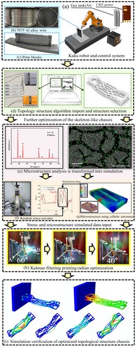
Table 2. Process and model parameters.

Parameter	Value	Ref.
Welding current(A)	116	–
Welding voltage(V)	13.4	–
Wire feed rate(m/min)	8.5	–
Travel speed(cm/min)	7.9	–
Airflow(L/min)	20	–
Heat source power Q (W)	1163	–
Heat source parameters af = ar, b, c(µm)	3,4,5	–
Ambient and initial temperature Ta, T0 (K)	25,80	–
Heat transfer coefficient h (W/(m^2 . K))	0.02	–
Density	${\rho }_w\left(T\right)=2830-0.513\cdot T+2\times {10}^{-4}\cdot T^2$	[28]
Thermal conductivity (W/m·K)	$k_w\left(T\right)=130.5+0.0161\cdot T-6\times {10}^{-6}\cdot T^2$	[28]
Specific heat (J/kg·K)	$\begin{array}{cc}{C}_w\left(T\right)=960& +0.53\cdot T-6\times {10}^{-6}\cdot T^2\\ & +6.2\times {10}^{-7}\cdot T^3\end{array}$	[28]
Young’s Modulus (MPa)	$E_w\left(T\right)=73431-123.35\cdot T+0.0517\cdot T^2$	[28]
Distribution coefficient	0.1	[29]
Liquid specific heat(T)	632.38	Jmatpro®
Solid specific heat	435	–
Latent heat	397000	Jmatpro®
Liquid diffusion coefficient $D_l\left(m^2/\mathrm{s}\right)$	3.0×10^−9	[29]
Gibbs-Tompson coefficient $\mathrm{\Gamma }\left(\mathrm{m}.\mathrm{K}\right)$	2.0e-07	[29]
Liquidus slope $\mathrm{m}\left(\mathrm{K}/\mathrm{w}\mathrm{t}\text{\%}\right)$	−60.95	[29]
Liquidus Temperature	632.38	Jmatpro®
Solid Temperature	459.07	Jmatpro®
Alloy initial composition (wt%)	5.09	Jmatpro®
Mean nucleation undercooling(fusion boundary nucleation) $\mathrm{\Delta }{T}_N^f\left(\mathrm{K}\right)$	11.4	–
Nucleation density$n_{max,S}\left(m{m}^{-2}\right)$	1.4×10^8	[29]
Cellular automata cell size Δx (µm)	3	–
Standard deviation of undercooling$\mathrm{\Delta }{T}_{\sigma }(\mathrm{K})$	0.5	–
Degree of the anisotropy of the interfacial energy, ϵ	0.3	[30]
Thermal expansion coefficient(K)	2.32×10^− 5	[31]

3. Mathematical model

3.1. Simple model topology generation

For the chassis structures produced by PIX Moving and other power-switching chassis structures, the maximum equivalent force is experienced at the connection between the battery compartment and the suspension support base substrate. Additionally, considering the challenges posed by complex road conditions, the overall load on the chassis is three-dimensionally variable. Therefore, in order to enable the unmanned vehicle chassis to adapt to the diverse and unknown loads encountered on actual roads, subdivision algorithms are employed on the chassis structure. This ensures that the chassis structure has maximum load-bearing capacity in both two-dimensional and three-dimensional spatial directions, as illustrated in Figure 2.

Figure 2. (a) Connecting nodes with potential truss members (b) Using optimisation to determine the best structural layout.

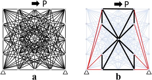
The optimal layout of a randomly generated structure is determined based on the given support conditions, loads, and discrete pivot points. This is because manufacturing constraints, such as the number of hollows in the prints and print lengths, have a significant impact on the specific stiffness of the optimised model [32]. Additionally, the structure is designed to ensure that the planar nodes are subjected to the maximum applied loads and that the node connections align with the optimal solution of Equation (1) [33], as shown below: (1) $\begin{array}{c}\begin{array}{c}\underset{\mathit{a},\mathit{q}}{min}V={\tilde{\mathit{l}}}^{T}a\\ \mathrm{s}.\mathrm{t}.\\ \begin{array}{c}B{\mathit{q}}^k={\mathit{f}}^k\\ {\mathit{q}}^k\ge -{\sigma }^{-}a\\ {\mathit{q}}^k\le {\sigma }^{+}a\\ a\ge 0\end{array}\}\mathrm{f}\mathrm{o}\mathrm{r}k=1,2,\dots ,p\end{array}\end{array}$(1) The volume of the structure is denoted by V. The area vector of each connecting line in the cross-section direction is represented by a = [a₁,a₂, … , a_m]^T. To prevent the infinite expansion of the generated structure, the maximum increase in the length of the required branch lines is preset as s. The length vector of each connecting line is denoted by l = [l₁+s,l₂+s, … ,l_m+s]^T. The equilibrium matrix B is a 2n×m matrix, where n is the number of nodes and m is the number of connecting lines. The internal force vectors of all the struts are represented by q, and k is the load case identifier. The total number of loads in Figure 2(a) and (b) is denoted by p. The Figure 2(b) diagram illustrates a simple example of chassis generation for a vehicle model. This diagram combines the axial load control rule to optimise the beam cell structure [34]. The external load vector is represented by f, and σ⁺ and σ^- denote the tensile and compressive stresses.

3.2. Material generation limitations

To ensure maximum load capacity while considering structural simplification, it is paramount to have the lowest cost of a structural connection that can withstand the maximum additional load. In this scenario, the adaptive layout optimisation algorithm of trusses [33] suggests using the maximum shape variability as an intermediary, combining both the simplification and load capacity factors in series, as shown below: (2) $\begin{array}{c}{ϵ}_i=\sum _{k=1}^p{\displaystyle \frac{max\left\{{\sigma }^{+}{\mathit{B}}_i^T{\mathit{u}}_i^k,-{\sigma }^{-}{\mathit{B}}_i^T{\mathit{u}}_i^k\right\}}{{\tilde{l}}_i}\le 1\left(fori=1,\dots ,m\right)}\end{array}$(2) The sum of the maximum virtual deformations of all generated spurs, denoted as ε_i, should be less than l under the interaction of the maximum tensile and maximum compressive stresses inside the pipe. The virtual displacement of the spurs with no additional structural generation cost, u_i^k, plays a role in this condition. When a single rod is incrementally increased or decrementally decreased in the structural generation, there is a cause for it. This also implies that increasing a potential single rod in the fixed space will enhance the overall generated structural loading capacity. Equation (1) represents a simplified set of members, but it still generates the full virtual displacement field for all nodes, u_k. If a violation of Equation (2) is found in the virtual displacement field, the most violating potential members can be added to Equation (1). The material generation constraints are then solved again to generate an improved virtual displacement field, where the newly added members no longer violate Equation (1) with Equation (2). This adaptive material generation rule process continues until no violations are detected.

3.3. Material occupancy

The purpose of this calculation is to determine the number of pixels within a rectangular graphic measuring 35 × 54 pixels, using the current two-dimensional chassis diagram. The material occupancy ratio is defined as the proportion of pixel points in the chassis model with greyscale values below 80 to the total pixel points in the 35 × 54 rectangular graphic. This ratio can also be interpreted as the relative area of the shaded portion. To begin, the chassis colour must be transformed into a greyscale image. Colours are made up of the primary colours red, green, and blue. Assuming the original colour of a point is RGB (R, G, B), we can convert it to a grey value using the following method: (3) $\begin{array}{c}\mathrm{G}\mathrm{r}\mathrm{a}\mathrm{y}={\displaystyle \frac{\left(R\times 30+G\times 59+B\times 11\right)}{100}}\end{array}$(3) The colours of the red, green, and blue channels are represented by RGB. To convert to greyscale value, the original RGB values (R, G, B) are replaced with a unified greyscale value, resulting in a new colour RGB (Grey, Grey, Grey). By replacing the original RGB values (R, G, B) with the new colour, a greyscale image can be obtained, as shown in the material occupancy below: (4) $\begin{array}{c}MO={\displaystyle \frac{G}{TPV}}\end{array}$(4) MO is the material occupancy rate, G is grey value, TPV is total pixel value, and the material occupancy rate of each iteration is shown in Figure 4.

3.4. Moving heat source

In this study, we adopted the double ellipsoid heat source model [35] to represent the equivalent heat source along an arbitrary free curve forming path. According to this model, the heat source moves along the x’ axis and the equations describing the front and back of the double ellipsoid are used: (5) $\begin{array}{c}\{\begin{array}{cc}& q\left(x^{\mathrm{\prime }},y^{\mathrm{\prime }},z^{\mathrm{\prime }}\right)=\\ & {\displaystyle \frac{6\sqrt{3}Q{f}_{\mathrm{f}}}{\pi \sqrt{\pi }{a}_{\mathrm{f}}bc}\exp \left(-3\left({\left({\displaystyle \frac{x^{\mathrm{\prime }}}{a_{\mathrm{f}}}}\right)}^2+{\left({\displaystyle \frac{y^{\mathrm{\prime }}}{b}}\right)}^2+{\left({\displaystyle \frac{z^{\mathrm{\prime }}}{c}}\right)}^2\right)\right),{\mathrm{x}}^{\mathrm{\prime }}>0}\\ & q\left(x^{\mathrm{\prime }},y^{\mathrm{\prime }},z^{\mathrm{\prime }}\right)=\\ & {\displaystyle \frac{6\sqrt{3}Q{f}_{\mathrm{r}}}{\pi \sqrt{\pi }{a}_{\mathrm{r}}bc}\exp \left(-3\left({\left({\displaystyle \frac{x^{\mathrm{\prime }}}{a_{\mathrm{r}}}}\right)}^2+{\left({\displaystyle \frac{y^{\mathrm{\prime }}}{b}}\right)}^2+{\left({\displaystyle \frac{z^{\mathrm{\prime }}}{c}}\right)}^2\right)\right),{\mathrm{x}}^{\mathrm{\prime }}<0}\end{array}\end{array}$(5) The local coordinates of a point with respect to the heat source are denoted as x’, y’, and z’. The semiellipsoid has characteristic lengths a, b, and c along the x, y, and z axes, respectively. The subscripts f and r represent the anterior and posterior ellipsoids, respectively. The fractions of heat source power (Q) in the anterior and posterior portions of the heat source are defined as f_f= 2/(1+a_r/a_f) and f_r= 2/(1+a_f/a_r). The thermal energy input per unit length to the weldment (line energy) Q is expressed as: (6) $\begin{array}{c}Q={\displaystyle \frac{\eta IU}{v}}\end{array}$(6) η is the thermal efficiency; U is the welding voltage; v is the welding speed(mm/s).

3.5. Dendrite growth theory

3.5.1. Thermal field calculations

The governing equation for transient heat transfer [36,37] is given by Eq: (7) $\begin{array}{c}\rho C_{\mathrm{p}}{\displaystyle \frac{\mathrm{\partial }T}{\mathrm{\partial }t}=\mathrm{\nabla }\cdot \left(\lambda \mathrm{\nabla }T\right)+\rho \mathrm{\Delta }H{\displaystyle \frac{\mathrm{\partial }{f}_{\mathrm{s}}}{\mathrm{\partial }t}}}\end{array}$(7) where T is the temperature, t is the time, ρ is the density, C_p is the specific heat, f_s is the solid phase fraction, λ is the thermal conductivity, and ΔH is the latent heat of solidification.

3.5.2. Dendrite growth calculation

At the S_L interface, the solute partitioning between liquid and solid is calculated by equation [36]: (8) $\begin{array}{c}{C}_{\mathrm{s}}=k{C}_1\end{array}$(8) The partition coefficient (k) represents the ratio between the solid and liquid phase interfacial components (C_s and C_l, respectively). As stated in Equation (8), the dendrites that grow reject solute at the S_L interface. The calculation of solute diffusion in the entire region is determined using this information [36]: (9) $\begin{array}{c}{\displaystyle \frac{\mathrm{\partial }{C}_i}{\mathrm{\partial }t}=\mathrm{\nabla }\cdot \left(D_i\mathrm{\nabla }{C}_i\right)+C_i\left(1-k\right){\displaystyle \frac{\mathrm{\partial }{f}_{\mathrm{s}}}{\mathrm{\partial }t}}}\end{array}$(9) In the equation, C represents the composition, D represents the solute diffusion coefficient, and the subscripts i denote solid or liquid. The second term on the right side of the equation accounts for the solute expelled at the S_L interface. To address the issue of nature discontinuity at the S_L interface, the equivalent composition C_e and the equivalent diffusion coefficient D_e are introduced in solving Equation (9), as defined in [36].

For the liquid phase: (10) $\begin{array}{c}{C}_{\mathrm{e}}=C_1,D_{\mathrm{e}}=D_1\end{array}$(10) For the solid phase: (11) $\begin{array}{c}{C}_{\mathrm{e}}={\displaystyle \frac{C_{\mathrm{s}}}{k},D_{\mathrm{e}}=D_{\mathrm{s}}}\end{array}$(11) For the interface: (12) $\begin{array}{c}{C}_{\mathrm{e}}=C_1,D_{\mathrm{e}}=D_1\end{array}$(12) Solid–liquid interface: (13) $\begin{array}{c}{D}_{\mathrm{e}}=D_{\mathrm{s}}\end{array}$(13) Between the interface and the liquid: (14) $\begin{array}{c}{D}_{\mathrm{e}}=D_{\mathrm{l}}\end{array}$(14) The local curvature κ and the local interface orientation ϕ are represented by Equation (13, 14) respectively. f(θ,ϕ) quantifies the surface energy anisotropy based on the preferred orientation ϕ in relation to the solid grain's θ (where θ = 0 represents grains aligned with the lattice orientation) [38]: (15) $\begin{array}{rl}& \kappa ={\left({\left({\displaystyle \frac{\mathrm{\partial }{f}_s}{\mathrm{\partial }x}}\right)}^2+{\left({\displaystyle \frac{\mathrm{\partial }{f}_s}{\mathrm{\partial }y}}\right)}^2\right)}^{-{\displaystyle \frac{3}{2}}}\\ & \left(2{\displaystyle \frac{\mathrm{\partial }{f}_s}{\mathrm{\partial }x}{\displaystyle \frac{\mathrm{\partial }{f}_s}{\mathrm{\partial }y}{\displaystyle \frac{{\mathrm{\partial }}^2{f}_s}{\mathrm{\partial }x\mathrm{\partial }x}-{\left({\displaystyle \frac{\mathrm{\partial }{f}_s}{\mathrm{\partial }x}}\right)}^2{\displaystyle \frac{{\mathrm{\partial }}^2{f}_s}{\mathrm{\partial }{y}^2}-{\left({\displaystyle \frac{\mathrm{\partial }{f}_s}{\mathrm{\partial }y}}\right)}^2{\displaystyle \frac{{\mathrm{\partial }}^2{f}_s}{\mathrm{\partial }{x}^2}}}}}}\right)\end{array}$(15) (16) $\begin{array}{c}\varphi ={\cos }^{-1}\left[{\displaystyle \frac{\mathrm{\partial }{f}_s}{\mathrm{\partial }x}{\left({\left({\displaystyle \frac{\mathrm{\partial }{f}_s}{\mathrm{\partial }x}}\right)}^2+{\left({\displaystyle \frac{\mathrm{\partial }{f}_s}{\mathrm{\partial }y}}\right)}^2\right)}^{-{\displaystyle \frac{1}{2}}}}\right]\end{array}$(16) (17) $\begin{array}{c}f\left(\theta ,\varphi \right)=1-\delta \cos \left(4\left(\varphi -\theta \right)\right)\end{array}$(17)

These equations indicate that growth will be inhibited in regions with high values of κ, as a result of the influence of surface energy on interfacial supercooling. The extent of this influence is determined by f(θ,ϕ), with the latter being more pronounced at interfacial sites where ϕ deviates significantly from θ. The anisotropy parameter δ in Equation (15) is a fixed value that quantifies the importance of the difference between ϕ and θ in the computation of f(θ,ϕ) [36,39,40]. (18) $\begin{array}{c}{C}_S={\displaystyle \frac{f_s{C}_S^{\ast }+\mathrm{\Delta }{f}_s{C}_S^{eq}}{f_s+\mathrm{\Delta }{f}_s}}\end{array}$(18) After calculating the amount of solidification according to Equation (8), an updated solids concentration C_S is then determined by considering the previous solids concentration C_S and the C_S^eq calculated in the cell. The change in the dissolved mass S [38] is used to calculate the amount of change. (19) $\begin{array}{c}S=C_L\left(1-k\right)\mathrm{\Delta }{f}_s\end{array}$(19) It is added to or subtracted from the local C_L. The calculated Δf_s is added to the current value of f_s in all cells simultaneously.

3.6. Kalman filter algorithm

The scanning speed of the robotic arm is constant, and the initial printing speed is set to 0.01 m/s in the Abaqus subroutine. In this study, we are primarily interested in the effect of the robotic arm's printing attitude on the printed structural parts, rather than the localised buildup in the printing melt pool. To simulate the print cross-section tissue distribution, we collect meso-microstructure images of different printing sites, which are designed as rectangles. These images are then used for the subsequent threshold calculation of image dendrite distribution and solute distribution. Following the approach of Derekar et al. [41], we establish a relationship between the print stress and the print angle to investigate how changes in the robotic arm's angle affect the print stress, which is distinct from the contouring method used to determine residual stress [41]. Similar to the Hierholzer algorithm [42] with constraints used to generate continuous printing paths, the robotic arm printing process in this study is real-time printing. Before exporting the SRC file, the printing process should be optimised by considering the organisation condition of the printed cross-section and the change in the stress state. Additionally, the motion of the molten pool is considered as a combination of homogeneous straight-line motion and random perturbation. 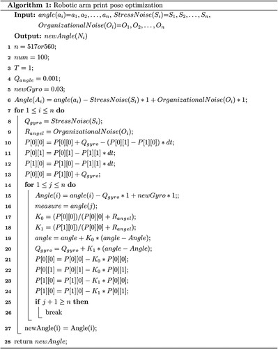The printing optimisation model can be expressed as follows: (20) $\begin{array}{c}\begin{array}{c}Angle=angle+Q_{bias}\cdot \mathrm{\Delta }t+newGyro\cdot \mathrm{\Delta }t\\ Q_{bias}=Q_{gyro}=StressNoise\left(S_i\right)\\ newGyro=OrganizationalNoise\left(O_i\right)\end{array}\end{array}$(20) The pseudo-code of the specific optimisation algorithm is presented in Figure 3. To account for the negative correlation effect of stress under high arc change, a negative sign is added in front of StressNoise(S_i). Additionally, since the cross-section organisation state factor and the print stress change factor change dynamically during the printing process, a Kalman filter-based tracking method is employed to accurately determine the position of the robotic arm's printing attitude. This allows for the capture and processing of the current print local region. The variables used in the algorithm are as follows: Q_angle represents the robotic arm noise covariance, Q_gyro represents the stress noise covariance, R_angle represents the optimised angular fine-crystal rate, Angle represents the optimised angle value, angle represents the value of the robotic arm printing angle to be optimised, StressNoise(S_i) represents the product of the print stress covariance and the angular speed of the robot arm A6-axis print. OrganizationalNoise(S_i) denotes the product of the percentage of grain boundaries and high solute regions and the angular speed of the robot arm A6-axis print, and the sampling period Δt is set to 1.

Figure 3. Pseudo-code of Kalman filtering algorithm.

4. Results and discussion

4.1. Generative chassis structure selection

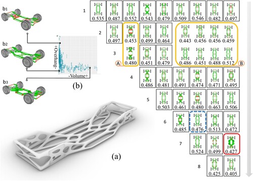
In order to understand the pickup process during the iterative optimisation, we present the design variables guided by the player following the topology generation and material constraints strategy in the game, as depicted in Figure 4. The entire optimisation process is implemented in the grasshopper platform using the industrial software Rhinoceros. Through topology generation rules, numerous basic bone-like chassis can be formed, resembling natural systems that react to loads and constraints [43]. However, the robotic arm carrying the arc printing device cannot print overhead due to the complex structure of the local bone-like chassis. We consider this constraint and highlight the part of the chassis robotic arm that overhangs during printing with red lines. Additionally, based on the controlled material printing rules (illustrated with green lines), we co-deploy them into a model scenario, as shown in Figure 4. Among many model scenarios, we present 44 optimised scenarios where the robotic arm does not overhang during printing and consumes the minimum amount of welding filaments. To analyze each model scenario with 100% material occupancy (indicated in green), we utilise the Image function in the Python Imaging Library (PIL). In Figure 4, for the 1st round of iteration selection (Player 1: 0.535, 0.487, 0.552, 0.543, 0.479, 0.509, 0.546, 0.482, 0.497), it is evident that the 9 model scenarios have more internal structural design variants with higher material layups, resulting in their higher material occupancy (green line) (5 molding solutions above 0.5), as observed in the graphical position occupied by model b₃ in Figure 4. Consequently, these scenarios were eliminated from the competition. Arriving at the second and third rounds (Player 2: 0.497, 0.453, 0.499, 0.464, 0.443, 0.456, 0.456, 0.459; Player 3: 0.480, 0.451,0.479, 0.486, 0.451, 0.488, 0.512), the boxed orange regions (A, B) are typical representatives. Region A is eliminated due to its excessive number of mechanical arm overhanging print segments (red lines), as shown in the diagrammatic position occupied by model b₁ in Figure 4. Region B is also eliminated due to its local structural complexity and too little lay-up material (e.g. material occupancy of 0.443, 0.451), which is not conducive to the final printing process. It is also eliminated because when printing complex surfaces with a large inclination, the molten filament would be affected by the angle of the surface and gravity, resulting in too much localised dimensional deviation. Similarly, rounds 4 and 5 selections were eliminated before the final round. Players 6, 7, and 8 (Player 6: 0.485, 0.476, 0.513, 0.472; Player 7: 0.524, 0.499, 0.427; Player 8: 0.425, 0.405) survived the last rounds, with player 7's red box selection being eliminated due to its excessive material spread and small material occupancy ( = 0.427) in localised portions of the green region, which showed a moderate amount of grey portions recognised by the Image function. Additionally, we observed that in the last round, we might have chosen the design variant that looks similar because of its smallest material occupancy and simpler structure. However, upon scrutiny, we can see that the red horizontal line represents the horizontal overhanging print of the robotic arm and the hollow structure is not conducive to the placement of the other body parts, leading to its elimination. Therefore, participant 6 is declared the winner of the competition (blue region). Participant 6 has a lower material occupancy and the least number of robotic arm overhang print lines, while still meeting the actual vehicle manufacturing requirements, such as the region where model b₂ of Figure 4 is located. This allows us to achieve the desired structure of the chassis shape, as shown in Figure 4(a).

Figure 4. Skeleton chassis structure iteration: (a) Optimal frame chassis; (b) Objective space: b₁ denotes high overhang and low volume capacity chassis; b₂ denotes low overhang and low volume capacity chassis; b₃ denotes low overhang and high volume capacity chassis;(1–8) vehicle iteration cycle sequence and its material occupancy rate; A denotes high overhang area; B denotes area with local structural complexity and too little lay-up material; Red area denotes chassis with redundancy lay-up material; Blue area denotes (a) and b₂.

4.2. Optimise the selected chassis local printing radian

4.2.1. Phase structure

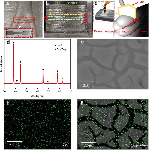
To refine the print area of the chosen chassis hub, we undertook a phase structure analysis of the 7075 aluminium alloy print. The results of the XRD analysis of the deposited samples in the deposition direction are presented in Figure 5(a). Figure 5(b,d) shows that the 7075 as-deposited sample in the horizontal orientation with deposition direction has α-Al as the matrix phase and MgZn₂ as the reinforcing phase [44]. Nucleation in the GP region occurs at temperatures ranging from 107 to 120 °C for several hours, followed by the formation of MgZn₂ precipitation at temperatures of 160 to 170 °C. At the scale of 2.5 $\mu m$, the distribution of equiaxed grain boundaries, observed by SEM, and the distribution of Zn element, observed by EDS compositional maps, can indicate the distribution of MgZn₂ both in the equiaxed grain boundaries and within the crystals, as shown in Figure 5(e,f,g). As the aging time increases, the precipitated phase grows and hinders dislocation motion, resulting in an increase in strength. However, if the size of the precipitated phase exceeds a critical value, dislocation motion tends to occur, leading to a decrease in strength. The results indicate that the presence of small-sized η′ phases enhances the strength of the alloy [45], and this strengthening mechanism is attributed to precipitation hardening caused by the formation of nanoprecipitates.

Figure 5. (a) Printing layer 150 cutting area and stretching sample; (b) the printing direction is approximated to the printing layers 150 and 200; (c) local diagram of the printing position; (d) XRD patterns of the 7075 aluminum alloy; (e) SEM image of the 7075 aluminum alloy showing distribution of equiaxial crystal; (f) EDS compositional maps of Zn in the selected region; (g) EDS compositional maps of MgZn₂ in the selected region.

4.2.2. Tensile properties

The specific size and location of the tested samples are illustrated in Figure 5(a). Tensile tests were conducted on the deposited specimens in both the deposition direction and horizontal direction (Figure 5(a,b)) to assess their macroscopic mechanical properties. In the horizontal direction, the average tensile strength was 358.64 MPa, the average yield strength was 196.15 MPa, and the average elongation was 37.9%. In the deposition direction, the average tensile strength was 269.29 MPa, the yield strength was 140.65 MPa, and the elongation was 32.52%. The test results of specimens with different orientations exhibited significant dispersion, particularly in elongation. This suggests that the deposited samples lack homogeneity. Furthermore, the average yield strength and ultimate strength in the horizontal direction were 24.91% and 26.03% higher, respectively, compared to the deposition direction.

4.2.3. The initial temperature

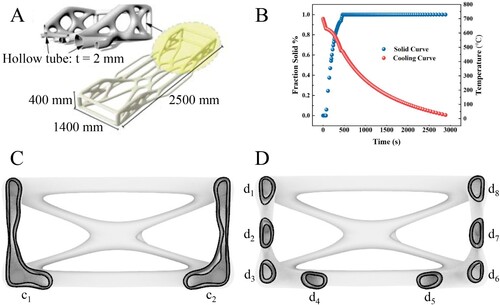
To accurately simulate the radian alterations of the robotic arm during the printing of the automotive body at the critical 150th and 200th layers, it is imperative to ascertain the printing temperature for the block substrate at the preceding 149th and 199th layers. According to Figure 6(B), by inputting the material composition parameters of the aluminum alloy, we can determine the relationship between the solid phase fraction of the alloy and the solidification time, as well as the relationship between the solidification temperature and time. The 149th layer has 560 print points, with a printing time of 2 s per point. On the other hand, the 199th layer has 517 print points, with a printing time of 1 s per point. The reason for different printing times is to prevent localised flow and hump phenomena while reducing the overall printing time through various experiments. Consequently, the total printing time for the 150th layer is 1120 s, while the total printing time for the 200th layer is 1034 s. Additionally, we assume that the c₁ and c₂ regions of the 150th layer are symmetric and independent of each other. This means that the temperatures in these two regions do not affect each other during the printing process. Based on this assumption, we can calculate that the total time for each c₁ and c₂ print area is 560 s (Figure 6(C)). Once the printing of the c₁ region is completed and the printing of the c₂ region begins, the internal pre-printing temperature of the 149th layer below the c₂ region is set to 430°C, which is determined based on the cooling trend shown in Figure 6(B). Similarly, we assume that regions d1-d8 in Figure 6 (D) are independent of each other, with the respective temperatures of d₁:63, d₂:70, d₃:60, d₄:65, d₅:65, d₆:60, d₇:70, and d₈:64. After printing the seven regions d₆-d₇-d₈-d₁-d₂-d₃-d₄, the pre-printing temperature inside this region was 500°C when the robotic arm returned to the d₅ region above the endpoint of the 149th layer printing for the 150th layer printing. The measurement error was validated using an indirect calculation method. A block was cut from the chassis near the 150th layer (Figure 5(a)), and three random points on the 150th layer were selected for measuring the residual stress values. In the Abaqus pre-processing, the substrate temperature was set to 430°C, and a print simulation was conducted to determine the residual stress simulation values for the three-point locations on the current printed layer. The error range between the measured residual stress simulation values and the actual values was found to be within 8%.

Figure 6. (A) Chassis structure size; (B) Alloy cooling trend; (C) The specific shape of the 150th printing layer; (D) The specific shape of the 200th printing layer.

4.2.4. Printing without radian change

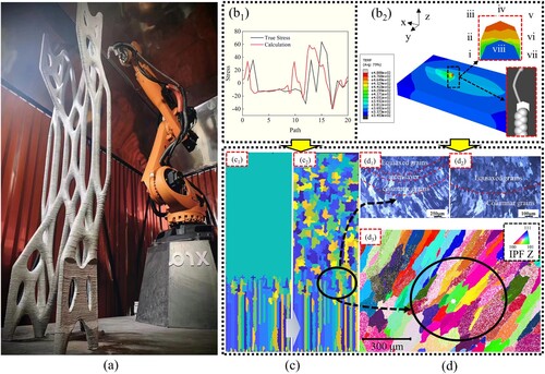
In order to improve the overall performance of the printed structural member (Figure 7(a)), mechanical simulations were conducted on a simulated t-shaped specimen. The simulations were carried out using a robotic arm without any change in attitude, and the grain structure at the printing position was analyzed (Figure 7). From Figure 7(b₁), it can be observed that the simulated residual stresses align with the changes in residual stress values observed in experimental tests. The stress values change from tensile to compressive and then back to tensile as the path progresses from Path1 to Path15. This indicates that a smaller temperature difference between the print layers tends to result in compressive stresses, while a larger temperature difference tends to lead to tensile stresses. Compressive stresses are generated at the melting site [46], during the cooling stage, both the melting zone and the heat-affected zone will undergo shrinkage. Additionally, the shrinkage of the liquid metal will transition from compressive stress to high tensile stress, particularly in the melting zone [47]. The characteristic morphological features of the phase structure described in subsections 4.2.1 are clearly visible in this analysis. The same grain growth mechanism is observed during the solidification of the first layer in the horizontal part of the t-shaped specimen. Figure 7(d₁, d₂) illustrates the distribution of meso-microscopic metallographic organisation after anodic coating. It is evident that there is a noticeable delamination phenomenon in the organisation. The process of printing macro-microscopic simulation is depicted from Figure 7(b₂) to Figure 7(c). In Figure 7(b₂), the (x,y,z) coordinates represent the printing angle of the tool head, while the ⅰ-ⅷ points indicate the 8 points selected for macro-printing. Figure 7(c) presents the meso-microscopic simulation of these 8 points using the CA-FE model. The CA-FE model follows the classical grain selection rule, where grains that are better aligned in the direction of heat flow/gradient are more abundant compared to relatively poorly aligned grains. As shown in Figure 7(c), both experiments and simulations reveal the growth of columnar grains parallel to the thermal gradient direction. Moving from Figure 7(c) to Figure 7(d), it can be observed that there is a distinct bottom-up transition between equiaxed α-Al grains and columnar α-Al grains in each layer. The delamination zone primarily consists of equiaxed dendritic tissues in the upper part, while the interlayer tissues are composed of columnar dendrites. Due to significant dendritic segregation, only the equiaxed dendritic morphology is observed in the top region, which is accompanied by nanoparticles precipitate in various regions, distributed in columnar and equiaxed crystals(Figure 5(g)). Figure 7(d) presents a detailed analysis of the microstructural characteristics of the isometric and columnar a-Al grain bands in the multilayer deposited samples. The presence of nanoprecipitates is also confirmed by the different orientations of the Z IPF grains (Figure 7(d₃)), which have an average aspect ratio of 1.32 and an average grain area of 386 μm². These grains exhibit a slight inclination in the deposition direction. In Figure 7(d₁), the bound intermediate layers between two consecutive layers show well-aligned grains in the tectonic direction, allowing them to survive and grow further. On the other hand, the new interlayer grains formed in Figure 7(d₂) are misaligned and tend to overgrow after a few hundred micrometers. The simulation setup involves arc scanning perpendicular to the substrate, with the scanning direction from left to right and subsequent layers from right to left. This results in a symmetric grain structure, where the grain boundaries in the block align with the build direction (Figure 7). The overall morphology pattern observed in the simulation is in good agreement with experimental observations, and the macroscopic form of the product is depicted in Figure 7(a).

Figure 7. (a) Kuka robot with a print chassis; (b₁) the comparison between the real residual stress and the simulated residual stress of the first layer of the printed block without radian change of the wire feed A6 axis; (b₂) welding wire feed A6 axis without radian change single-layer printing simulation and temperature section in YZ plane direction; (c) c₁ denotes the planar growth process of two-dimensional microstructure was simulated based on CA in (b₂, Simulation process: 42%); c₂ denotes simulation end state in (b₂, Simulation process: 100%); (d) d₁ denotes longitudinal tissue characteristics(250 µm); d₂ denotes longitudinal tissue characteristics at high magnification(100 µm); d₃ denotes IPF diagram in Z direction.

4.2.5. Printing radian microscopic changes

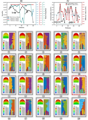
When the tool head of the robotic arm changes its radian in space, it comes into contact with argon at room temperature in the opposite direction of printing. Additionally, the thermal history of the entire deposition process can directly influence the grain structure and size distribution of the printed layers 150 and 200 [48]. To simulate the actual printing state, the arc change values of the 150th and 200th layers are incorporated into the first layer using the Abaqus subroutine. Additionally, the temperature distribution of the 149th and 199th layers is predicted based on the printing time and utilised as the base layer temperature in Abaqus. This allows for a better simulation of the printing state of the actual chassis with the block material. In subsection 4.2.4, the analysis focuses on the real-time and spatial constraints of the robotic arm during the printing process. The arc printing angle continuously changes throughout the process. This subsection specifically analyzes the 150th and 200th layers. The 150th layer has 560 print changes, corresponding to 560 print points, while the 200th layer has 517 print changes, corresponding to 517 print points. Each layer is sampled in batches, with 20 points taken as the main features of each segment. The print changes of the 150th and 200th layers are inputted as an array of Abaqus subroutines, and the simulation is carried out for a print segment of 200 mm in length. The simulation was conducted under a printing segment of 200 mm. The simulation results of the printing stresses and the mesomicrocosmic simulation results of the corresponding positions are shown in Figures 8 and 9. It can be observed that when printing from the end of the bone-like chassis to the 150th layer, the printing radius of the robotic arm is positively correlated with the changes of the B and C axes within the range of 0.2 Rad, and is not affected by the changes of the A-axis printing radius. However, when printing to the Path100 mm, as shown in Figure 8Ⅰ, the A-axis changes by −0.87, the B-axis changes positively by about 0.07 Rad, and the C-axis changes by −1.1 Rad, resulting in a drastic increase in printing stresses. The reason for this is that when printing an arc from above to below, the compressive stress disappears and the arc energy is dumped in the upward direction, leading to more fusion defects and porosity in the specimen [49]. The impact on the already printed region below is relatively less. At the position of the Path130, there is a localised surge in stress. This is because the printing of larger parts results in a reverse direction temperature difference that affects the change in compressive stress, as shown in Figure 8(a.b). According to the self-developed threshold algorithm in Figure 8(c), the solute distribution and dendrite state were calculated for each meso-microscopic picture. The grey value of the grain boundary and the solute region were determined by calculating the pixel points. By accumulating the pixel points of the solute grey value and the grain boundary grey value, the proportion of the grain boundary and the high solute region were determined. A higher grain boundary rate, closer to 1, indicates a more homogeneous structure of dendrites and higher grain boundary density. However, it should not be too close to 1, as the calculation may mistake the convergence at the same pixel site for solute aggregation. On the other hand, a lower grain boundary rate, closer to 0.2, suggests a lower solute aggregation and indicates the extent to which the simplified two-dimensional region of the growth and decomposition model of the precipitated phases may appear in the region [50]. To regulate the uniform distribution of the organisation and improve the dendritic structure and solute distribution, it is recommended to aim for a grain boundary rate of 0.5, based on the principle of maximisation of Cauchy's inequality. Figure 9 illustrates the change in attitude under the organisation morphology, with the best grain boundary rate observed in the position Path70 mm (Figure 8Ⅱ). During the competitive growth process shown in Figure 8 (7), the crystal growth direction is controlled by aligning with the direction of the local maximum temperature gradient, which is antiparallel to the direction of the (outward) normal to the melt pool boundary [51]. At this moment, the precipitated phase is most uniformly distributed, and the dendrites tilt from rightward to leftward during the same solidification time from Figure 8(1) to Figure 8(5). The solute aggregation increases and then decreases, while the solute aggregation decreases from upward to homogenisation from Figure 8(7) to Figure 8(9). In Figure 8(7) to Figure 8(10), the dendrite is tilted to the right from the left, resulting in an increase and then a decrease in solute aggregation. Moving on to Figure 8(10) to Figure 8(15), the dendrite is tilted to the left until it reaches a parallel position with the two dendrites, causing a decrease in solute aggregation bias followed by aggregation. From Figure 8(15) to Figure 8(20), the dendrite exhibits a slight tilt in the middle, leading to a significant solute aggregation. During this time, the amplitude of the A-axis increases gradually, while the other axes remain unchanged. This indicates that when the tool head is perpendicular to the change in the block plane, larger solute aggregation may occur. Therefore, it is important to avoid uniaxial changes. The changes in the axes print are approximately −0.20886, −0.00351, and −0.20794, respectively. Similarly, when the robotic arm prints up to 200 layers, the print stress remains within 0.2 Rad of the print angle change in the C-axis. Additionally, the print stress shows a positive correlation, and there is a surge in print stress locally when the C-axis change magnitude is −1.6 Rad, specifically at positions a, b, and c in Figure 9III. Similarly, in Figure 9(1–20), the degree of solute aggregation fluctuates, starting high and then decreasing. This fluctuation is caused by the simultaneous change of the A-axis and B-axis. Furthermore, there is a tendency for aggregation within a 1 Rad change and a lower aggregation within a 1 Rad-1.6 Rad change. In Figure 9, the Ⅳd position indicates the current printing position with the best microstructure morphology. At the Path150 mm position, the radian change is optimal, with each axis changing by −0.08757, 0.002843, and −0.08356 radians. The organisational state at this position is shown in Figure 9 number 15, where the distribution of the small-size η′ phase is the most uniform compared to other mesomorphic simulation maps. This indicates that the dimensional accuracy on the local 2D scale is closer to the original CAD model [52].

Figure 8. Ⅰ the print stress change under the change of space radian A, B and C of the A6 axis of the robotic arm in the 150th layer; Ⅱ grain boundary rate change and difference change diagram in the 150th layer(absolute difference with 0.5); (1–20) microstructural changes in the 150th layer(average of 20 segments).

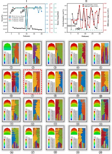
Figure 9. Ⅲ the print stress change under the change of space radian A, B and C of the A6 axis of the robotic arm in the 200th layer; Ⅳ grain boundary rate change and difference change diagram in the 200th layer(absolute difference with 0.5); (1–20) microstructural changes in the 200th layer(average of 20 segments).

4.2.6. Kalman filter optimisation

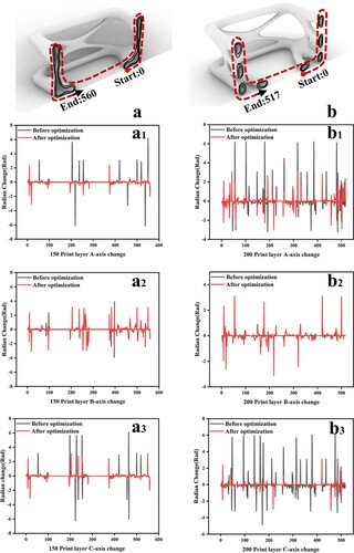
By analyzing the collected print stress sequences and image sequences along with the results of the analysis in subsection 4.2.5, it can be observed that this aligns with the concept of Kalman filtering [53]. Kalman filtering is known for its ability to filter and fit data that contains noise and inaccuracies, allowing for a more accurate estimation of unknown variables. This finding suggests that applying Kalman filtering can help reduce local stress surges and improve tissue morphology. Additionally, considering the similarity between the impact angle and the arc filament feed angle, the impact angle does not have a statistically significant effect on the layer thickness of the material [54]. Therefore, the impact of print layer collapse on Kalman filter print arc optimisation is not taken into account. The connection points of the link sub-paths may potentially be weak nodes [55]. To mitigate this, sequential printing of sub-paths a and b, as shown in Figure 10, is adopted to reduce printing weak points. Furthermore, based on the results of subsection 4.2.5, the stress and tissue rate are transformed into modulation angles corresponding to the arc change. The original printing change angle, stress noise, and tissue distribution noise are used as inputs for the Kalman filter to effectively filter stress surges and excessive solute aggregation regions. This enables more precise localisation of the 3D rotational arc position of the printed melt pool, as depicted in parts a, a₁, and a₂ of Figure 10. In the optimisation of the 150th layer's A-axis, tissue regulation is primarily focused on at the beginning of the printing stage, while stress regulation is observed in the 200–280 region and tissue regulation in the 380–560 region for the B-axis. The C-axis is associated with a reduction in tissue rate in the 190–280 region and the 380–560 region, as well as a reduction in stress rate in the 380–560 region. To reduce the changes in arc caused by stress surges and changes in tissue solute bias, the 380–560 region is targeted. Similarly, the main changes occur in the 200th layer of the A and C axes, while the optimisation effect is consistent with the comprehensive embodiment of synergistic optimisation of print stress and tissue control in the 150th layer of the C-axis. This is depicted in Figure 10 b₂, and b₃, with the B-axis shown in Figure 10 b₁. The main purpose of the B-axis is to control the tissue solute control of the tiny attitude changes caused by the large bias and dendrite coarse large bias polymerisation and dendrite coarsening while performing attitude regulation of the robotic arm. In summary, the unchanged region must be accurately printed in order to ensure that the melt pool maintains a low-stress effect on the previous print layer and finer tissue characteristics after solidification. The filtering results are shown in Figure 10. The original change angle of 0 Rad can be modified to ± 2Rad through the optimisation of the Kalman filter. Additionally, in order to reduce printing stress, the range of change in radians for the position with larger change angles has been reduced from 4–6Rad to 0.2 Rad-2 Rad. As shown in Figure 10, the A-axis path points and the C-axis path points below the print layer 150 achieve a reduction in the value of the A and C radians of the robotic arm's A6 axes by a factor of 20: a₁(55–60), a₁(195–200), a₁(215–220), a₁(230–240), a₁(415–425), a₁(460–470), a₁(490–500), a₁(490–500), a₁(530–540), a₁(545–555); a₃(50–60), a₃(50–60), a₃(415–425), a₃(460–470), a₃(490–520). An increase in the value of the arm A6 axis B radian is achieved at the B-axis path points below the print layer 150, with a 20-fold magnitude increase: a₂(0–30), a₂(190–280), a₂(420–560). An increase in the value of the A and B radians of the robotic arm A6 axis is observed at the A-axis path point and the B-axis path point below the print layer 200, with a 20-fold magnitude increase: b₁(0–50), b₂(0–517). A decrease in the value of the C-axis curvature of the robotic arm A6-axis C is observed at the C-axis path point below the print layer 200, with a 20-fold magnitude decrease: b₃(30–210), b₃(250–400). The reduction of the robotic arm A6 axis A radian value to 1/3 is achieved at the A-axis path points below print layer 200: b₁(50–200), b₂(320–360). Overall, the printing radian change has increased up to 20 times compared to the original, due to the change in the rate of organisation change. Furthermore, the arc changes have decreased to 1/3 of the original value as a result of printing stress changes.

Figure 10. (a) denotes print layer 150 printing direction;a₁ denotes comparison of robotic arm printing angle A before and after optimisation in print layer 150;a₂ denotes comparison of robotic arm printing angle B before and after optimisation in print layer 150;a₃ denotes comparison of robotic arm printing angle C before and after optimisation in print layer 150; (b) denotes print layer 200 printing direction;b₁ denotes comparison of robotic arm printing angle A before and after optimisation in print layer 200;b₂ denotes comparison of robotic arm printing angle B before and after optimisation in print layer 200;b₃ denotes comparison of robotic arm printing angle C before and after optimisation in print layer 200.

4.3. Macro performance simulation tests

4.3.1. Unmanned vehicle chassis crash and organizational analysis

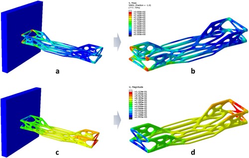
Macroscopic finite element simulation tests were conducted on the optimised prints to analyze the behaviour of the chassis during a collision with a fixed deformable barrier at a high initial velocity (v = 40 km/h). The collision results in the conversion of kinetic energy of the chassis into internal energy of the structure within a very short time. This internal energy interaction is reflected in the structure through transient stress and local displacement changes, as depicted in diagrams (Figure 11(a- b)). The impact energy is transmitted from the head to the tail, leading to a uniform distribution of Von Mises Stress over a large area, with stress vectors aligned with the edges of the hollow holes [56]. The Von Mises Stress in the tail is approximately 75 MPa, indicating a localised rise in energy in that region. It is worth noting that the maximum local displacement of the structure occurs at the tail rather than the head, which can be attributed to its unique bionic structure. The maximum local displacement at the tail is measured to be 0.1 mm. Additionally, the interaction between printing layers (automobile wheel area) contributes to effective stress wave transmission relief, as observed in Figures 11 c and d.

Figure 11. Simulation of chassis impact stresses: (a) lateral face stress change; (b) frontal stress change; Simulation of chassis local deformation: (c) lateral face deformation; (d) frontal deformation.

4.3.2. Unmanned vehicle chassis modal analysis

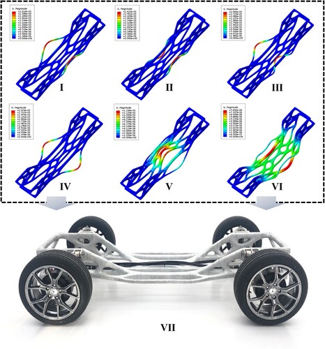
The present study focuses on the modal vibration mode and vibration frequency of a multi-degree-of-freedom system, specifically the chassis structure. It should be noted that the simulation does not account for nonlinear contact connections such as friction contact, frictionless contact, or rough contact. The number value of eigenvalues requested is 30 in Abaqus. Figure 12 illustrates the eigenvalues and frequencies of the skeletal chassis for the first six vibration modes: Mode I: 1.13, 0.169 Hz; Mode II: 1.45, 0.17 Hz; Mode III: 2.31, 0.24 Hz; Mode IV: 2.31, 0.242 Hz; Mode V: 2.41, 0.24 Hz; Mode VI: 2.81, 0.26 Hz. It is observed that the vibration patterns of the first four orders only involve changes in the external edge trusses, indicating a safer body structure. However, the centre of the vibration patterns for the fifth and sixth orders shift significantly, suggesting a more precarious body structure. Figure 12 Ⅶ showcases the product iteration achieved through the aforementioned method.

Figure 12. Ⅰ→Ⅵ: the first six modes of vibration of the chassis mode; Ⅶ:optimised skeleton chassis.

5. Summary

This research presents a comprehensive framework that combines numerical simulation and experimental characterisation to significantly reduce the chassis design, iteration, and validation cycles. The principal findings are as follows:

1. At the design stage, we implemented the ‘adaptive member addition’ algorithm and adhered to material restriction rules to generate a diverse set of 44 topological chassis structures. Through rigorous selection, we identified a skeletal body with the lowest material occupancy (0.427) and leveraged OpenCV image processing to effectively prevent overhanging prints.

2. For optimisation, we created a 20 dm block print based on the block printout to enhance the efficiency of the skeletal body’s printing process. Our study indicates that the tissue distribution and stress patterns of the robotic arm concur closely with simulation data absent attitude printing variations. We also examined the impact of various attitude changes on robotic arm printing, finding a direct relationship between printing stress and C-axis variations within a 0.2 Rad range. Beyond a 1.1 Rad change, significant simultaneous alterations in the A-axis and B-axis were observed, suggesting a convergence tendency within a 1 Rad range and reduced convergence from 1 Rad to 1.6 Rad. Isolated changes in axis A must be avoided. It is essential to maintain each axis’s change within a maximum of 0.2 Rad to control tissue morphology and solute distribution. Kalman filtering was successfully applied to adjust radian changes in stress surge regions and enhance radian changes in high tissue rate areas. Consequently, printing radian changes have increased up to 20 times due to organisational rate changes and decreased to a third of their original value due to printing stress alterations.

3. In the validation phase, collision simulations at speeds of up to 40 km/h indicated that our optimised printed structure sustained minimal deformation, with a maximum deviation of only 0.1 mm. The eigenvalues and frequencies of the bone-like chassis at each vibration order were as follows: I: 1.13, 0.169 Hz; II: 1.45, 0.17 Hz; III: 2.31, 0.24 Hz; IV: 2.31, 0.242 Hz; V: 2.41, 0.24 Hz; VI: 2.81, 0.26 Hz.

This methodology enables the automotive chassis design and manufacturing iteration cycle to be completed within just one week, representing a 120-fold reduction in the development cycle. The framework is applicable to nearly all robotic arm-based 3D printing strategies and provides an initial foray into microstructure-based 3D printing processes, facilitating real-time optimisation of the robotic arm printing process. Nonetheless, it is noteworthy that the framework is not yet seamlessly integrated into the robotic arm control system, primarily due to the extensive simulation time required. Furthermore, addressing the microstructure of the 7075 aluminum alloy under varying process parameters remains a challenge, as traditional experimental and computational methods fall short. To surmount these hurdles, we aim to adopt a data-driven approach in our subsequent research.

Disclosure statement

No potential conflict of interest was reported by the author(s).

Data availability statement

The data that support the findings of this study are available from the corresponding author upon reasonable request.

Additional information

Funding

This work was supported by Guizhou Provincial Program on Commercialization of Scientific and Technological Achievements (QKHCG[2023] general 083).

References

- Gibson I, Rosen D, Stucker B. Additive manufacturing technologies: 3D printing, rapid prototyping, and direct digital manufacturing. Cham: Springer; 2015.
- Thompson MK, Moroni G, Vaneker T, et al. Design for additive manufacturing: trends, opportunities, considerations, and constraints. CIRP Ann. 2016;65(2):737–760. doi:10.1016/j.cirp.2016.05.004
- Vaneker T, Bernard A, Moroni G, et al. Design for additive manufacturing: framework and methodology. CIRP Ann. 2020;69(2):578–599. doi:10.1016/j.cirp.2020.05.006
- Aage N, Andreassen E, Lazarov BS, et al. Giga-voxel computational morphogenesis for structural design. Nature. 2017;550(7674):84–86. doi:10.1038/nature23911
- Smith CC, Gilbert M, et al. Application of discontinuity layout optimization to plane plasticity problems. P Roy Soc A-Math Phy. 2007;463:2461–2484. doi:10.1098/rspa.2013.0009
- Wang Z, Zhang Y, Bernard A, et al. A constructive solid geometry-based generative design method for additive manufacturing. Addit Manuf. 2021;41:101952. doi:10.1016/j.addma.2021.101952
- Wang YQ, Wang A. On the topological yarn structure of 3-D rectangular and tubular braided preforms. Compos Sci Technol. 1994;51(4):575–586. doi:10.1016/0266-3538(94)90090-6
- Wu J, Aage N, Westermann R, et al. Infill optimization for additive manufacturing-approaching bone-like porous structures. Ieee T Vis Comput Gr. 2018;24(2):1127–1140. doi:10.1109/TVCG.2017.2655523
- Guo X, Zhang W, Zhong W. Doing topology optimization explicitly and geometrically—a new moving morphable components based framework. J Appl Mech. 2014;81(8):081009. doi:10.1115/1.4027609
- Bai J, Zuo W. Hollow structural design in topology optimization via moving morphable component method. Struct Multidiscip O. 2020;61(1):187–205. doi:10.1007/s00158-019-02353-0
- Zhang W, Yu TX, Xu J. Uncover the underlying mechanisms of topology and structural hierarchy in energy absorption performances of bamboo-inspired tubular honeycomb. Extreme Mech Lett. 2022;52:101640. doi:10.1016/j.eml.2022.101640
- Jayanath S, Achuthan A. A computationally efficient finite element framework to simulate additive manufacturing processes. J Manuf Sci E-T Asme. 2018;140(4). doi:10.1115/1.4039092
- Rai A, Helmer H, Körner C. Simulation of grain structure evolution during powder bed based additive manufacturing. Addit manuf. 2016: 13. doi:10.1016/j.addma.2016.10.007
- Lu L-X, Sridhar N, Zhang Y-W. Phase field simulation of powder bed-based additive manufacturing. Acta Mater. 2018;144:801–809. doi:10.1016/j.actamat.2017.11.033
- Rodgers TM, Madison JD, Tikare V. Simulation of metal additive manufacturing microstructures using kinetic Monte Carlo. Comp Mater Sci. 2017;135:78–89. doi:10.1016/j.commatsci.2017.03.053
- Zinovieva O, Zinoviev A, Ploshikhin V. Three-dimensional modeling of the microstructure evolution during metal additive manufacturing. Comp Mater Sci; 141:207–220. doi:10.1016/j.commatsci.2017.09.018
- Liu J, To AC. Quantitative texture prediction of epitaxial columnar grains in additive manufacturing using selective laser melting. Addit Manuf. 2017;16:58–64. doi:10.1016/j.addma.2017.05.005
- Rappaz M, Gandin C-A. Probabilistic modelling of microstructure formation in solidification processes. Acta Metall Mater. 1993;41:345–360. doi:10.1016/0956-7151(93)90065-Z
- Gandin CA, Rappaz M, Tintillier R. Three-dimensional probabilistic simulation of solidification grain structures: application to superalloy precision castings. Metall Trans A. 1993;24(2):467–479. doi:10.1007/BF02657334
- Koepf JA, Soldner D, Ramsperger M, et al. Numerical microstructure prediction by a coupled finite element cellular automaton model for selective electron beam melting. Comp Mater Sci. 2019;162:148–155. doi:10.1016/j.commatsci.2019.03.004
- Lian Y, Gan Z, Yu C, et al. A cellular automaton finite volume method for microstructure evolution during additive manufacturing. Mater Des. 2019;169(6):107672. doi:10.1016/j.matdes.2019.107672
- Zinoviev A, Zinovieva O, Ploshikhin V, et al. Evolution of grain structure during laser additive manufacturing. Simulation by a cellular automata method. Mater Des. 2016;106:321–329. doi:10.1016/j.matdes.2016.05.125
- Kaji F, Jinoop AN, Zardoshtian A, et al. Robotic laser directed energy deposition-based additive manufacturing of tubular components with variable overhang angles: adaptive trajectory planning and characterization. Addit Manuf. 2023;61(7):103366. doi:10.1016/j.addma.2022.103366
- Guidetti X, Balta EC, Nagel Y, et al. Stress flow guided non-planar print trajectory optimization for additive manufacturing of anisotropic polymers. Addit Manuf. 2023;72(5):103628. doi:10.1016/j.addma.2023.103628
- Huang Y, Fang G, Zhang T, et al. Turning-angle optimized printing path of continuous carbon fiber for cellular structures. Addit Manuf. 2023;68:103501. doi:10.1016/j.addma.2023.103501
- Jin Y-a, He Y, Fu J-z, et al. Optimization of tool-path generation for material extrusion-based additive manufacturing technology. Addit Manuf. 2014;1-4:32–47. doi:10.1016/j.addma.2014.08.004
- Bartlett JL, Croom BP, Burdick J, et al. Revealing mechanisms of residual stress development in additive manufacturing via digital image correlation. Addit Manuf. 2018;22:1–12. doi:10.1016/j.addma.2018.04.025
- Wu Q, Li D-P. Analysis and X-ray measurements of cutting residual stresses in 7075 aluminum alloy in high speed machining. Int J Precis Eng Man. 2014;15(8):1499–1506. doi:10.1007/s12541-014-0497-4
- Kim M-S, Lee S-H, Jung J-G, et al. Prediction of grain structure in direct-chill cast Al–Zn–Mg–Cu billets using cellular automaton-finite element method. Prog Nat Sci-Mater. 2021;31(3):434–441. doi:10.1016/j.pnsc.2021.05.003
- Song Y, Jiang H, Zhang L, et al. Integrated model for describing the microstructure evolution of the inoculated Al-Zn-Mg-Cu alloys in continuous solidification. Results Phys. 2021;26(2):104465. doi:10.1016/j.rinp.2021.104465
- Sun J, Hensel J, Köhler M, et al. Residual stress in wire and arc additively manufactured aluminum components. J Manuf Process. 2021;65:97–111. doi:10.1016/j.jmapro.2021.02.021
- Fernandes RR, van de Werken N, Koirala P, et al. Experimental investigation of additively manufactured continuous fiber reinforced composite parts with optimized topology and fiber paths. Addit Manuf. 2021;44(15):102056. doi:10.1016/j.addma.2021.102056
- He L, Gilbert M, Song X. A Python script for adaptive layout optimization of trusses. Struct Multidiscip O. 2019;60(2):835–847. doi:10.1007/s00158-019-02226-6
- Xia L, Bi M, Wu J, et al. Integrated lightweight design method via structural optimization and path planning for material extrusion. Addit Manuf. 2023;62(10):103387. doi:10.1016/j.addma.2022.103387
- Mohebbi MS, Ploshikhin V. Implementation of nucleation in cellular automaton simulation of microstructural evolution during additive manufacturing of Al alloys. Addit Manuf. 2020;36:101726. doi:10.1016/j.addma.2020.101726
- Zhu M, Stefanescu D. Virtual front tracking model for the quantitative modeling of dendritic growth in solidification of alloys. Acta Mater. 2007;55(5):1741–1755. doi:10.1016/j.actamat.2006.10.037
- Meng G, Gong Y, Zhang J, et al. Multi-scale simulation of microstructure evolution during direct laser deposition of Inconel718. Int J Heat Mass Transfer. 2022;191:122798. doi:10.2139/ssrn.4017183
- Rolchigo MR, LeSar R. Modeling of binary alloy solidification under conditions representative of additive manufacturing. Comp Mater Sci. 2018;150:535–545. doi:10.1016/j.commatsci.2018.04.004
- Zhang Y, Zhang J. Modeling of solidification microstructure evolution in laser powder bed fusion fabricated 316L stainless steel using combined computational fluid dynamics and cellular automata. Addit manuf. 2019: 28. doi:10.1016/j.addma.2019.06.024
- Chandra S, Tan X, Narayan RL, et al. A generalised hot cracking criterion for nickel-based superalloys additively manufactured by electron beam melting. Addit Manuf. 2020: 37. doi:10.1016/j.addma.2020.101633
- Derekar KS, Ahmad B, Zhang X, et al. Effects of process variants on residual stresses in wire arc additive manufacturing of aluminum alloy 5183. J Manuf Sci E-T Asme. 2022;144(7):1–35. doi:10.1115/1.4052930
- Yamamoto K, Luces JVS, Shirasu K, et al. A novel single-stroke path planning algorithm for 3D printers using continuous carbon fiber reinforced thermoplastics. Addit Manuf. 2022;55(2):102816. doi:10.1016/j.addma.2022.102816
- Zegard T, Paulino G. GRAND — ground structure based topology optimization for arbitrary 2D domains using MATLAB. Struct Multidiscip Optim. 2014;50:861–882. doi:10.1007/s00158-014-1085-z
- Hu Z, Xu P, Pang C, et al. Microstructure and mechanical properties of a high-ductility Al-Zn-Mg-Cu aluminum alloy fabricated by wire and arc additive manufacturing. J Mater Eng Perform. 2022;31(8):6459–6472. doi:10.1007/s11665-022-06715-6
- Park JK, Ardell AJ. Microstructures of the commercial 7075 Al alloy in the T651 and T7 tempers. Metall Trans A. 1983;14(10):1957–1965. doi:10.1007/BF02662363
- Luo Z, Zhao Y. A survey of finite element analysis of temperature and thermal stress fields in powder bed fusion additive manufacturing. Addit Manuf. 2018;21:318–332. doi:10.1016/j.addma.2018.03.022
- Cambon C, Bendaoud I, Rouquette S, et al. A WAAM benchmark: from process parameters to thermal effects on weld pool shape, microstructure and residual stresses. Mater Today Commun. 2022;33:104235. doi:10.1016/j.mtcomm.2022.104235
- Zhang J, Liou F, Seufzer W, et al. A coupled finite element cellular automaton model to predict thermal history and grain morphology of Ti-6Al-4V during direct metal deposition (DMD). Addit Manuf. 2016;11; doi:10.1016/j.addma.2016.04.004
- Fathi-Hafshejani P, Soltani-Tehrani A, Shamsaei N, et al. Laser incidence angle influence on energy density variations, surface roughness, and porosity of additively manufactured parts. Addit Manuf. 2022;50(11):102572. doi:10.1016/j.addma.2021.102572
- Yu Y, Kenevisi M, Yan W, et al. Modeling precipitation process of Al-Cu alloy in electron beam selective melting with a 3D cellular automaton model. Addit Manuf. 2020;36:101423. doi:10.1016/j.addma.2020.101423
- Teferra K, Rowenhorst D. Optimizing the cellular automata finite element model for additive manufacturing to simulate large microstructures. Acta Mater. 2021;213(6):116930. doi:10.1016/j.actamat.2021.116930
- Diourté A, Bugarin F, Bordreuil C, et al. Continuous three-dimensional path planning (CTPP) for complex thin parts with wire arc additive manufacturing. Addit Manuf. 2021;37:101622. doi:10.1016/j.addma.2020.101622
- Kalman RE. A new approach to linear filtering and prediction problems. J Basic Eng. 1960;82(1):35–45. doi:10.1115/1.3662552
- Nault IM, Ferguson G, Nardi A. Multi-axis tool path optimization and deposition modeling for cold spray additive manufacturing. Addit Manuf. 2020;38(3):101779. doi:10.1016/j.addma.2020.101779
- Wan Q, Yang W, Wang L, et al. Global continuous path planning for 3D concrete printing multi-branched structure. Addit Manuf. 2023;71(3):103581. doi:10.1016/j.addma.2023.103581
- Suzuki T, Fukushige S, Tsunori M. Load path visualization and fiber trajectory optimization for additive manufacturing of composites. Addit Manuf. 2019;31:100942. doi:10.1016/j.addma.2019.100942