A non-probabilistic convex modelling framework for uncertainty quantification of laser powder bed fusion fabricated structures based on limited data

ABSTRACT

Laser powder bed fusion (LPBF) is increasingly prominent in essential fields such as aerospace. However, due to the characteristics of the manufacturing process and the high test cost, the performance of fabricated structures is inherently uncertain, leading to a challenging characterisation of their performance. This paper proposes a non-probabilistic convex modelling framework involving confirming uncertainties, processing data, and establishing a non-probabilistic convex model, to quantitatively describe the uncertainties concerning the physical properties of structures fabricated by LPBF. Firstly, the non-probabilistic convex modelling framework is proposed and an efficient uncertainty quantification method is developed utilising the non-probabilistic convex model. Then, criteria are set up for evaluating the performance of the developed method, and computational efficiency and accuracy are illustrated via benchmark numerical examples. Last but not least, two types of representative structures, solid and lattice structures, are fabricated via the LPBF method. The physical properties are tested through tensile and compression experiments. By confirming the necessity of accounting for uncertainties with limited data, we employing the proposed framework to the real representative specimens fabricated via the LPBF method, demonstrating that the structures fabricated by LPBF have substantial uncertainty and the proposed framework is practical.

KEYWORDS:

• Non-probabilistic modelling
• convex model
• uncertainty quantification
• evaluation criterion
• laser powder bed fusion

1. Introduction

Due to its high porosity and unique periodic microstructure, novel structures, including lattice structures, honeycomb structures, metamaterials, etc., are characterised by high specific strength and specific stiffness, excellent vibration absorption, noise reduction, and heat dissipation [1–4]. These outstanding properties confer great application potential in various fields and received widespread attention from researchers and engineers [5–7]. To fabricate novel structures with porosity and periodic microstructure, additive manufacturing (AM), especially metal AM technology, is essential [8–10]. Laser powder bed fusion (LPBF) [11] is a powder-based layer-by-layer metal AM process, that can produce high-density metal parts with complex shapes and precise microstructures [12–14]. However, the LPBF’s quality of structures involves multiple factors [15], inevitably bringing uncertainties to the manufactured structures, including size, porosity, relative density, mechanical properties, and so on [16–18]. These uncertainties have a significant impact on the reliability evaluation, structural optimisation design, and improvement of manufacturing processes, and must be quantified through appropriate methods. However, due to the multiple factors involved and the high cost of testing, quantifying the uncertainties in the LPBF process becomes a challenge [19, 20]. In particular, these uncertainties have two main characteristics, namely, the uncertainties (1) are correlated and (2) vary with certain factors. Improper modelling of the uncertainties may result in misleading reliability analysis, which can increase the risk or cost of structural applications. Therefore, to apply novel structures manufactured by LPBF to practical engineering, there is an urgent demand for a framework to quantify the uncertainties accurately [21, 22].

The probabilistic and non-probabilistic methods are two common candidates for dealing with uncertainties. As a sophisticated approach, the probabilistic method has been deeply studied at the theoretic level and widely used to quantify various uncertainties in many engineering practices [23]. The probabilistic method is very mature for uncertain problems with enough information, while in contrast, the non-probabilistic method is an important alternative for uncertainty quantification with limited sample data. In recent years, the non-probabilistic method has been widely concerned and rapidly developed. Various models concerning non-probabilistic methods have emerged in the field of uncertainty analysis. Among them, the non-probabilistic convex model [24, 25], consisting of the multi-dimensional ellipsoid (ME) model [26] and multi-dimensional parallelepiped (MP) model [27], can take the correlation information into account and quantitatively describe the uncertainties using convex sets. In ME and MP models, the uncertainty domain of parameters is depicted as a multi-dimensional ellipsoid and a multi-dimensional parallelepiped, respectively. Conveniently, the degree of correlation between parameters is illustrated by the shape of the ellipsoid or parallelepiped, while the degree of uncertainty is presented by the geometry size [28]. Based on the non-probabilistic convex model, many achievements have been achieved in various fields [29–32], promoting the rapid development of uncertainty quantification and analysis.

The non-probabilistic convex model is suitable for quantifying uncertain-but-bounded parameters with limited sample data. At the same time, LPBF-fabricated structures involve multiple uncertainties caused by the manufacturing process and limited sample data due to high test costs. Therefore, the non-probabilistic convex model is a potentially effective approach to achieve the uncertainty quantification of LPBF-fabricated structures. Gorguluarslan et al. [33] proposed a methodology utilising the Bayesian information criterion for predicting the elastic behaviour of lattice structures processed by AM. Li et al. [34] presented a time-variant reliability analysis framework for predicting the lifetime of the SLM-fabricated structures with hybrid uncertainties. Lozanovski et al. [35] proposed a Monte Carlo simulation-based approach to predict the stiffness of additively manufactured lattice structures, aiming at reliability analysis of AM lattice structures. To predict the reliability without the explicit model of the physics behind the manufacturing process, Snider-Simon et al. [36] presented a novel workflow considering process parameters, building strategy, and test data to develop models of material microstructure. However, these studies were mainly devoted to establishing and applying reliability analysis models to LPBF-manufactured structures, while very few paid attention to developing novel uncertainty quantification and modelling approaches.

In this study, a non-probabilistic convex modelling framework is proposed to quantify uncertainties of LPBF-fabricated structures. Two types of representative structures are processed via LPBF utilising 316L and AlSi10Mg. The physical properties are tested to confirm the necessity of quantifying uncertainties with limited data. Then an efficient uncertainty quantification method is developed based on the non-probabilistic convex model. Numerical examples are provided with criteria established to evaluate the performance of the developed method. Furthermore, the proposed framework is compared with other state-of-the-art methods and subsequently applied to the LPBF fabricated representative structures.

The remainder is arranged as follows. Section 2 is devoted to developing the non-probabilistic convex modelling framework and the convex modelling processes. Section 3 establishes criteria for performance evaluation and conducts a comprehensive performance evaluation of the proposed framework. Section 4 provides comparisons with other convex modelling methods via examples and employs the proposed framework for uncertainty quantification of the LPBF-fabricated structures to verify the practicality and accuracy of the proposed framework. Subsequently, some conclusions and further discussions are given in Section 5.

2. Methods

The existing research evidently shows that structures fabricated by LPBF inherently involve uncertainties regarding physical properties. These uncertainties are challenging to be delicately depicted using traditional probabilistic models with limited experimental data. Thus, to quantitatively describe the uncertainties of LPBF-fabricated structures, a non-probabilistic convex modelling framework is proposed. As shown in Figure 1, the proposed framework mainly consists of three parts, i.e. (I) Confirming structural uncertainties, (II) processing model parameters, and (III) constructing a convex model, which will be detailed in the following.

Figure 1. The proposed non-probabilistic convex modelling framework for LPBF-fabricated structures.

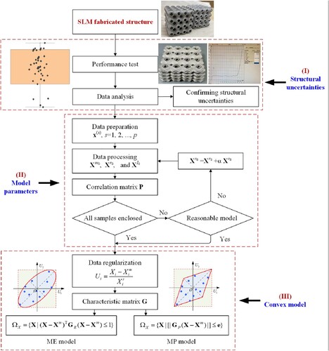
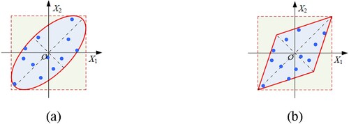
Suppose that X^(s), s = 1, 2, … , p, represents p sets of sample data extracted from experiments, referring to physical properties of structures fabricated by LPBF, which will be employed to quantify the uncertain-but-bounded parameters X = {X₁, X₂, … , X_n}^T. For the non-probabilistic convex model, these uncertain parameters can be described using an n-dimensional convex domain. Generally, the ME model is used to formulaically depict the uncertain-but-bounded parameters as shown in Figure 2(a), that is. (1) ${\mathrm{\Omega }}_X=\{\mathit{X}\in {\mathrm{R}}^p|(\mathit{X}-{\mathit{X}}^m{)}^{\mathrm{T}}{\mathit{G}}_E(\mathit{X}-{\mathit{X}}^m)\le 1\}$(1) where Ω_X represents the convex domain, and X^m= [X₁^m, X₂^m, … , X_n^m] is the vector of midpoint. G_E is called the characteristic matrix, which guarantees that Ω_X is bounded and determines the geometric characteristic of the ellipsoid. Similarly, the uncertain space of variables also can be described by using the MP model as shown in Figure 2(b), which can be formulated as (2) ${\mathrm{\Omega }}_X=\{\mathit{X}\in {\mathrm{R}}^p|\left[\right|{\mathit{G}}_P(\mathit{X}-{\mathit{X}}^m)\left|\right]\le \mathit{e}\}$(2) where G_P refers to the characteristic matrix determining the geometry of the parallelepiped and e is an n-dimensional unit vector marked as e = [1 1 … 1]^T.

Figure 2. The non-probabilistic convex models: (a) ME model and (b) MP model.

To construct the above convex models, the intervals of variables and the corresponding characteristic matrix should be acquired in advance. In most practical engineering, limited experimental samples are normally available, indicating that the intervals of variables should be appropriately determined. Based on the traditional methods and our previous work [37], the midpoints of the intervals can be expressed by using the mean values, as. (3) $X_i^m={\displaystyle \frac{1}{p}\sum _{s=1}^p{X}_i^s}$(3) where $X_i^s$ represents the experimental sample in the sth group referring to parameter X_i. The correlation coefficient between parameters, X_i and X_j, is formulated as (4) ${\rho }_{\mathrm{ij}}={\displaystyle \frac{{\sum }_{s=1}^p(X_i^s-X_i^m)(X_j^s-X_j^m)}{\sqrt{{\sum }_{s=1}^p{(X_i^s-X_i^m)}^2{\sum }_{s=1}^p{(X_j^s-X_j^m)}^2}}}$(4) Generally, aiming to determine the variation ranges of uncertain parameters, the convex model suitably surrounding all the sample points should be established at first. To avoid the influence of a few error data on the establishment of the convex model, accurately determining the variation ranges of uncertainties can be converted to the optimisation problem. That is, seeking the optimised convex model by adjusting or ignoring the error data. In this way, the established convex model’s geometric size is more economic and reasonable, which can minimise the impact of erroneous data. Herein, two indexes are introduced for the optimisation, including the inclusion ratio β and the cost ratio ξ, which are defined as. (5) ${\text{β}}_{p_{\mathrm{in}}}={\displaystyle \frac{p_{\mathrm{in}}}{p},\xi ={\displaystyle \frac{{\text{β}}_{p_{\mathrm{in}}}-{\text{β}}_{p_{\mathrm{in}}-1}}{V_{p_{\mathrm{in}}}^{\frac{1}{n}}-V_{p_{\mathrm{in}}-1}^{\frac{1}{n}}}}}$(5) where p is the sample size and p_in is the sample size surrounded by the convex model. ${\text{β}}_{p_{\mathrm{in}}}$ corresponds to the inclusion ratio when p_in sample points are included, and $V_{p_{\mathrm{in}}}$ is the volume of the convex model surrounding p_in sample points. Then, the optimisation problem for searching the optimised convex model can be formulated as (6) $\begin{array}{rl}& minV,\\ & \mathrm{s}.\mathrm{t}.X_i^m,i=1,2,\cdots ,n,\\ & {\rho }_{\mathrm{ij}},i,j=1,2,\cdots ,n,\\ & {\mathit{x}}^{\left(s\right)}\in {\mathrm{R}}^p,s=1,2,\cdots ,p,\\ & {\text{β}}_{p_{\mathrm{in}}}\ge {\text{β}}_0,\\ & \xi \le {\xi }_0.\end{array}$(6) where β₀ and ξ₀ are two parameter values defined according to the precision requirement. A large value of β₀ means a high model accuracy, but it can also cause an increase in model volume. The parameter ξ₀ reflects the balance between improving model accuracy and reducing model volume. In fact, the values of the two parameters can be adjusted according to the actual application situation. Based on the authors’ understanding and attempt of the model, it is recommended to choose the values of β₀ and ξ₀ as 0.95 and 0.005, respectively, to accommodate most situations. Considering that the radii of the parameter intervals determines the volume and that the ratio between the obtained interval and the actual interval of each parameter can be assumed to be approximately equal, Eq. (6)(6) $\begin{array}{rl}& minV,\\ & \mathrm{s}.\mathrm{t}.X_i^m,i=1,2,\cdots ,n,\\ & {\rho }_{\mathrm{ij}},i,j=1,2,\cdots ,n,\\ & {\mathit{x}}^{\left(s\right)}\in {\mathrm{R}}^p,s=1,2,\cdots ,p,\\ & {\text{β}}_{p_{\mathrm{in}}}\ge {\text{β}}_0,\\ & \xi \le {\xi }_0.\end{array}$(6) is equivalent to (7) $\begin{array}{rl}& min\alpha ,\\ & \mathrm{s}.\mathrm{t}.X_i^r=X_i^{r_0}+\alpha X_i^{r_0},i=1,2,\cdots ,n,\\ & X_i^m,i=1,2,\cdots ,n,\\ & {\rho }_{\mathrm{ij}},i,j=1,2,\cdots ,n,\\ & {\mathit{x}}^{\left(s\right)}\in {\mathrm{R}}^p,s=1,2,\cdots ,p,\\ & {\text{β}}_{p_{\mathrm{in}}}\ge {\text{β}}_0,\\ & \xi \le {\xi }_0.\end{array}$(7) where α is an increment coefficient, $X_i^r$ is the interval radius of the uncertain parameter X_i, and $X_i^{r_0}$ is the initial interval radius obtained from the interval of experimental samples. Eq. (7)(7) $\begin{array}{rl}& min\alpha ,\\ & \mathrm{s}.\mathrm{t}.X_i^r=X_i^{r_0}+\alpha X_i^{r_0},i=1,2,\cdots ,n,\\ & X_i^m,i=1,2,\cdots ,n,\\ & {\rho }_{\mathrm{ij}},i,j=1,2,\cdots ,n,\\ & {\mathit{x}}^{\left(s\right)}\in {\mathrm{R}}^p,s=1,2,\cdots ,p,\\ & {\text{β}}_{p_{\mathrm{in}}}\ge {\text{β}}_0,\\ & \xi \le {\xi }_0.\end{array}$(7) is a linear single-target optimisation problem and can be readily solved via a simple optimisation technique with linear convergence [38]. Hence, the optimisation process is of high efficiency and the computation result can have high accuracy by adjusting the iterative step size in the optimisation technique.

Solving the above optimisation problem, one can identify the intervals of uncertain-but-bounded parameters, and then the convex model depicting the uncertainty domain can be mathematically given. Thus, the whole procedure of constructing the non-probabilistic convex model is summarised as follows:

Step 1: Test the physical properties of LPBF-fabricated structures to acquire the sample data x^(s), s = 1, 2, … , p.

Step 2: After analysis, confirm the necessity of uncertainty quantification and identify the critical uncertain-but-bounded parameters.

Step 3: Process the data to obtain the mean value $X_i^m$ and radius $X_i^{r_0}$ of uncertain parameter X_i, i = 1, 2, … , n.

Step 4: Compute all the correlation coefficients ${\rho }_{\mathrm{ij}}$ between different parameters X_i and X_j to compose the correlation matrix P.

Step 5: By solving the presented optimization problem, determine the precise interval bounds of parameters $X_i^I$.

Step 6: In light of the correlation matrix P and the intervals $X_i^I$, construct the characteristic matrix G_E or G_P for the corresponding convex model.

Step 7: Based on the matrix G_E or G_P, write the mathematical expression to establish the convex model.

At this point, the proposed non-probabilistic framework can be fully established to measure the uncertainty of LPBF-fabricated structures. It should be noted that the proposed framework can obtain precise variation intervals of uncertain parameters based solely on limited actual data, and achieve the removal of error samples during the modelling process.

3. Performance evaluation

3.1.‏ Criteria establishment

To quantitatively evaluate the practical performance of the proposed framework, several criteria are established based on our previous work [37], including the prediction accuracy η reflecting the predictive performance of modelling methods for unknown data, volume ratio ζ and standard volume ratio $\overline{\zeta }$ indicating the economic benefits of modelling methods, (8) $\eta ={\displaystyle \frac{N_S}{N_T}\times 100\text{\%},\zeta ={\displaystyle \frac{V_C}{V_R}\times 100\text{\%},\overline{\zeta }={\zeta }^{\frac{1}{n}}}}$(8) where N_S is the sample size of test data in the established convex model, and N_T is the total sample size of test data. V_C and V_R represent the volumes of the established convex model and the corresponding hyper-rectangle model, respectively. The specific calculation of V_C and V_R can be referred to [39]. Generally, an excellent convex model is expected to have high prediction accuracy with a low standard volume ratio. That is, to obtain a convex model with high accuracy at a low cost in engineering. In this regard, a new criterion for comprehensively evaluating convex models can be defined as (9) $Q={\displaystyle \frac{\eta }{\overline{\zeta }}}$(9) where Q is the new criterion called cost performance. It can be observed from Eq. (9)(9) $Q={\displaystyle \frac{\eta }{\overline{\zeta }}}$(9) that a considerable value of Q represents an outstanding performance of a convex model containing both the prediction accuracy and standard volume ratio.

3.2. Performance evaluation

With the established criteria, it is convenient to concretely evaluate the performance of the convex modelling method under various conditions. Considering the potential situations in practical engineering, the sample data can be of different numbers, distributions, correlations, and even incorrect samples. Therefore, the capability of the proposed method in the three cases should be tested.

Firstly, to test the capability of the proposed method with different numbers of sample data, randomly generate p two-dimensional sample data from two uncertain variables, X₁ and X₂, for uncertainty quantification. Herein the value of p is assumed to be an integer from 10 to 90 to supply nine cases. Suppose the variables X₁ and X₂ obey the normal distribution with mean values ${\mu }_{X_1}={\mu }_{X_2}=100,$ and deviations ${\sigma }_{X_1}={\sigma }_{X_2}=10.$ The correlation coefficient is set as ρ =  0.5. By using the Pauta criterion [40], the interval of the variable obeying the normal distribution can be expressed as [μ−3σ, μ+3σ], that is [70, 130] for variables X₁ and X₂, which makes it easy to calculate the volume of the corresponding hyper-rectangle model. To balance the calculation efficiency and accuracy, the total sample size of the test data N_T is set as 10,000, and the mean value of 100 test results is accepted in each case.

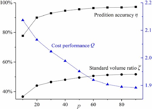
Figure 3 shows the performance of the established ellipsoid model under different sample sizes. It implies that even in small sample sizes, the established ellipsoid model can have superior performance, e.g. the prediction accuracy η = 77.65% under the condition p = 10 and η = 92.82% under the condition p = 30. Specifically, the prediction accuracy rises as the sample number increases and ultimately approaches 100%. The standard volume ratio increases with the sample size but remains below 100%, indicating that the space of the established model is smaller than that of the corresponding hyper-rectangle. In addition, under the combined effect of variations in prediction accuracy and standard volume ratio, the cost performance gradually decreases with the increase of the sample number but is greater than one. Thus, the proposed convex modelling method possesses outstanding performance when the sample data is limited.

Figure 3. Performance under different sample numbers.

Secondly, different correlations between two uncertain variables are considered to further study the performance of the proposed modelling method. Suppose that the two random variables X₁ and X₂ are generated under the condition that the correlation coefficient ρ are the following cases: (Ⅰ) ρ = 0.1; (Ⅱ) ρ = 0.2; (Ⅲ) ρ = 0.3; (Ⅳ) ρ = 0.4; (Ⅴ) ρ = 0.5; (Ⅵ) ρ = 0.6; (Ⅶ) ρ = 0.7; (Ⅷ) ρ = 0.8; (Ⅸ) ρ = 0.9. Similarly, the ellipsoid model is established by randomly employing 30 samples, and then 10,000 sample points are randomly created for performance testing. In each case, the mean value of 100 test results is adopted.

Figure 4 presents the test results of the established ellipsoid model under different correlations. It can be noticed that when other conditions remain unchanged, the correlation coefficients of variables will have a significant impact on the ellipsoid model, e.g. $\overline{\zeta }$ = 66.62% and Q = 1.40 when ρ = 0.1, and $\overline{\zeta }$ = 27.26% and Q = 3.50 when ρ = 0.9. In particular, while the fluctuation in prediction accuracy is not evident, the standard volume ratio and cost performance are markedly changed. The standard volume ratio decreases visibly with the correlation increasing, while the cost performance rises sharply as the correlation enhances. Consequently, the proposed convex modelling method can effectively handle uncertain variables with correlation, especially those with high correlation.

Figure 4. Performance under different correlations.

Finally, uncertain variables subject to two types of distribution, that is normal and uniform distributions, are discussed to evaluate the prediction capability. Assume that the centres and deviations of the normal distribution remain unchanged, and the uncertainty range of the uniform distribution is set as [90, 110]. The number of samples is p = 30, and the correlation coefficient is ρ = 0.5. Equally, 10,000 sample points are generated for testing, and the mean value of 100 test results is adopted in each condition.

The test results are presented in Table 1, in which the prediction accuracy of all established convex models exceeds 92%, and the standard volume ratio is less than one. Thus, it manifests that the proposed convex modelling method owns excellent performance in both the two kinds of distributions, demonstrating that the proposed convex modelling method possessing excellent generalisation ability.

Table 1. Test results under different sample distributions.

Model Type	Distribution	ƞ	$\overline{\zeta }$	Q
Ellipsoid	Normal	92.82%	46.50%	2.02
Parallelepiped	Normal	92.65%	48.76%	1.93
Ellipsoid	Uniform	94.07%	35.91%	2.64
Parallelepiped	Uniform	96.56%	35.87%	2.64

At the end of this subsection, it is worth emphasising that the established convex models can ignore some marginal sample points during the modelling process in the tests, which demonstrates the capability of preprocessing error data of the proposed method.

3.3. Efficiency and accuracy

The efficiency of the proposed framework mainly depend on modelling process, especially the calculation of the optimisation problem in Eq. (7)(7) $\begin{array}{rl}& min\alpha ,\\ & \mathrm{s}.\mathrm{t}.X_i^r=X_i^{r_0}+\alpha X_i^{r_0},i=1,2,\cdots ,n,\\ & X_i^m,i=1,2,\cdots ,n,\\ & {\rho }_{\mathrm{ij}},i,j=1,2,\cdots ,n,\\ & {\mathit{x}}^{\left(s\right)}\in {\mathrm{R}}^p,s=1,2,\cdots ,p,\\ & {\text{β}}_{p_{\mathrm{in}}}\ge {\text{β}}_0,\\ & \xi \le {\xi }_0.\end{array}$(7) , while other processes occupy little time. Without considering error sample points, the optimisation problem can be solved with linear convergence via the advanced-retreat method. The total number of the computational effort is q × l, where q is the number of experimental samples, l is the number of iterative steps.

In addition to the influencing factors analyzed in Section 3.2, the accuracy of uncertainty quantification in the proposed framework largely relates to the iterative step-size for solving the optimisation problem. The actual interval radius $X_i^r$ must be between two iterative steps, as. (10) $X_i^{r_0}+(l-1)\mu X_i^{r_0}<X_i^r\le X_i^{r_0}+\left(\mathrm{l\mu }\right)X_i^{r_0},i=1,2,\dots ,l$(10) where μ is the iterative step-size coefficient. According to Eq. (10)(10) $X_i^{r_0}+(l-1)\mu X_i^{r_0}<X_i^r\le X_i^{r_0}+\left(\mathrm{l\mu }\right)X_i^{r_0},i=1,2,\dots ,l$(10) , the accuracy of the solution satisfies the inequality written as (11) ${\text{β}}_a<{\displaystyle \frac{\left[X_i^{r_0}+\left(\mathrm{l\mu }\right)X_i^{r_0}\right]-\left[X_i^{r_0}+(l-1)\mu X_i^{r_0}\right]}{X_i^r}\le \mu }$(11) Thus, it can be observed that a small value of μ can achieve high accuracy of the solution. However, it also increases the number of iterative steps, which inevitably affects the computing efficiency. To balance the efficiency and accuracy of the solution, μ is generally recommended be to set to 0.01. In practical applications, the value of μ can be adjusted based on accuracy and efficiency requirements.

4. Results and discussions

To further verify the effectiveness of the proposed convex modelling framework, we will systematically compare the model established by the proposed framework with other advanced methods through benchmark numerical examples. Herein, two existing competitive convex models, namely the convex correlation coefficient-based (CCC-based) model and the sample correlation coefficient-based (SCC-based) model [39], are adopted. The CCC-based model heavily relies on the marginal sample points, while the SCC-based model focuses on the information of all samples. Therefore, these two models have advantages in different situations and are suitable for comparison with the new model. Then, through processing and testing of the practical structures, a complete uncertainty quantification process is conducted around the proposed framework for the LPBF-fabricated structures.

4.1. A two-dimensional uncertainty problem

A two-dimensional (2D) uncertainty quantification problem related to LPBF- fabricated structure is presented to validate the developed convex modelling method before embedding it into the proposed framework. Two uncertain variables X1 and X2 with their correlation ρ = 0.5 are considered to be described by using convex models with given 50 groups of samples. The 50 groups of samples are randomly generated in the intervals X1I = [90,110] and X2I = [90,110] with obeying uniform distribution, and the correlation between the two variables ρ = 0.5, as displayed in Table 2.

Table 2. Samples of X₁ and X₂ for convex modelling.

No.	X1	X2	No.	X1	X2	No.	X1	X2
1	97.51	94.31	18	99.05	106.13	35	104.20	96.46
2	103.60	102.14	19	106.29	102.92	36	102.97	103.74
3	107.47	106.91	20	105.13	102.68	37	101.84	106.79
4	103.06	94.83	21	98.33	103.38	38	104.04	99.31
5	93.69	94.19	22	103.60	97.37	39	100.18	102.09
6	99.55	96.14	23	96.78	101.88	40	97.38	104.93
7	102.08	98.45	24	96.80	96.03	41	92.33	97.45
8	100.39	98.78	25	96.87	100.10	42	101.24	102.28
9	94.48	92.68	26	92.69	99.79	43	94.95	97.97
10	96.55	97.60	27	106.43	100.44	44	95.31	92.86
11	107.49	104.83	28	102.86	97.17	45	94.62	92.71
12	104.54	101.99	29	95.91	105.16	46	100.08	94.27
13	106.67	99.90	30	99.96	99.24	47	92.58	96.98
14	97.67	101.67	31	104.47	101.81	48	99.56	106.31
15	95.53	101.28	32	98.16	101.43	49	93.02	99.87
16	102.77	95.43	33	95.67	101.17	50	99.11	106.04
17	97.78	98.45	34	103.43	100.13

Applying the proposed method for uncertainty quantification, the mean values and radii of the two parameters can be acquired as $X_1^m=99.73$, $X_2^m=99.93$ and $X_1^{r_0}=7.76$, $X_2^{r_0}=7.25$. Then calculating the correlation coefficient and the correlation matrix P can be written as. (12) $\mathit{P}=\left[\begin{array}{cc}1& 0.3304\\ 0.3304& 1\end{array}\right]$(12) Utilising the mean values, radii, and correlation matrix to model the optimisation problem and solve it to acquire the precise variation intervals of the parameters as $X_1^I=[91.43,108.03]$ and $X_2^I=\left[92.17107.69\right]$. Based on the correlation matrix and variation intervals, the characteristic matrix G_E or G_P can be constructed. Finally, the ellipsoid model and the parallelepiped model quantifying the uncertain parameters can be comfortably constructed. And for comparison, the CCC-based model and the SCC-based model are also established. Figure 5 intuitively shows the two types of convex models for describing the uncertainty using different modelling methods. Table 3 provides the key parameters of the convex models with t being the time consumption for convex modelling.

Figure 5. Convex models: (a) Ellipsoid models and (b) Parallelepiped models.

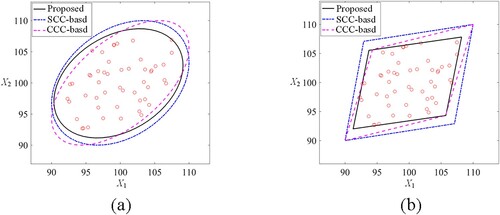
Table 3. Parameters related to the performance of the models.

Type	Model	ζ	$\overline{\zeta }$	t	X^m
Ellipsoid	Proposed	61.03%	78.12%	0.296	[99.73 99.93]
	CCC-based	64.56%	80.35%	0.292	[100 100]
	SCC-based	74.12%	86.09%	0.373	[100 100]
Parallelepiped	Proposed	48.27%	69.48%	0.305	[99.73 99.93]
	CCC-based	56.92%	75.44%	0.301	[100 100]
	SCC-based	70.91%	84.21%	1.135	[100 100]

It can be found that, based on the given 50 samples, the model constructed by the proposed method has a smaller volume while enclosing all the provided samples, with its better performance demonstrated compared with the others. Additionally, in terms of time consumption, the outstanding modelling efficiency of the proposed method is also revealed. Therefore, this 2D problem has confirmed the suitability and accuracy of the proposed method for uncertainty problems with limited data.

4.2. A cantilever beam

Consider a typical three-dimensional cantilever beam, as shown in Figure 6, where its free end is subjected to a combined action of a concentrated horizontal force Fx = 50,000N and a concentrated vertical force Fy = 25,000N. To ensure the load-bearing safety, the maximum stress on the beam must be less than the yield stress σS. Based on the knowledge of mechanics, the maximum stress of the cantilever beam occurs at its fixed end. The limit state equation can be expressed as. (13) $g(b,w,l)={\sigma }_S-{\displaystyle \frac{6F_{x}l}{w^{2}h}-{\displaystyle \frac{6F_{y}l}{w{h}^2}}}$(13) where l, w and h are the length, width and height of the cantilever beam, respectively. Due to the existence of processing errors, the geometric dimensions of the cantilever beam are not fixed values in actuality but fluctuate within a small range. Thus, the geometric parameters should be treated as uncertain variables and appropriate uncertainty quantification need to be conducted. Herein, 34 samples containing two error samples far from the centre are available, as listed in Table 4.

Figure 6. A cantilever beam.

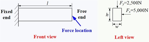
Table 4. Samples of geometric parameters of the cantilever beam [41].

No.	w	h	l	No.	w	h	l
1	97.69	206.31	926.14	18	105.90	207.54	990.00
2	94.41	199.87	957.64	19	94.24	187.77	961.88
3	102.21	190.99	1021.50	20	106.43	200.40	979.21
4	102.93	210.95	951.07	21	103.22	186.30	959.35
5	93.51	193.42	963.15	22	105.62	196.03	1067.4
6	106.17	203.32	1045.33	23	94.18	200.84	987.31
7	100.86	202.23	1041.28	24	101.87	187.02	1037.59
8	103.90	193.14	954.14	25	98.08	187.99	978.36
9	95.97	208.08	974.42	26	95.36	202.15	991.77
10	103.81	207.95	1069.66	27	98.54	198.42	1023.88
11	101.98	196.86	1019.12	28	104.58	190.56	1023.37
12	97.08	198.40	974.78	29	95.62	205.75	1042.84
13	101.32	202.56	956.40	30	98.44	198.11	993.78
14	99.18	208.92	943.92	31	102.26	202.30	1056.27
15	98.01	214.03	992.20	32	103.18	195.30	931.20
16	94.87	191.42	1024.99	33	108.25	219.41	1198.25
17	91.83	196.72	965.26	34	82.13	182.26	901.57

Firstly, applying the proposed method to establish the convex model for uncertainty quantification, the mean values and radii of the uncertain parameters can be obtained as $w^m=99.52$mm, $h^m=199.22$mm and $l^m=997.21$mm and $w^{r_0}=17.39$mm, $h^{r_0}=20.19$mm and $l^{r_0}=201.04$mm. Then we calculate the correlation coefficients between the three parameters in pairs to form the correlation matrix P, which can be written as. (14) $\mathit{P}=\left[\begin{array}{ccc}1& 0.0285& 0.2973\\ 0.0285& 1& -0.0203\\ 0.2973& -0.0203& 1\end{array}\right]$(14) Based on the mean values, radii, and correlation matrix of the parameters, modelling the optimisation problem and solving it to determine the precise interval bounds of parameters. Herein, the variation intervals of the geometric parameters can be acquired as $w^I=[90.16,109.42]$mm, $h^I=[181.06,217.16]$mm and $l^I=[902.26,1085.56]$mm. According to the correlation matrix and the acquired variation intervals, the characteristic matrix G_E or G_P can be constructed. Finally, the ME model and MP model quantifying the geometric parameters with uncertainties can be mathematically formulated.

The ME model can be expressed as. (15) $\begin{array}{rl}& {\left[\begin{array}{c}(w-99.79)/9.63\\ (h-199.11)/18.05\\ (l-993.91)/87.11\end{array}\right]}^{\mathrm{T}}{\left[\begin{array}{ccc}1& 0.0285& 0.2973\\ 0.0342& 1& -0.0203\\ 0.2973& -0.0203& 1\end{array}\right]}^{-1}\\ & \left[\begin{array}{c}(w-99.79)/9.63\\ (h-199.11)/18.05\\ (l-993.91)/87.11\end{array}\right]\le 1\end{array}$(15) The MP model can be expressed as (16) $\left[\left|{\left[\begin{array}{ccc}0.8565& 0.0131& 0.1304\\ 0.0148& 0.9741& -0.0111\\ 0.1308& -0.0099& 0.8593\end{array}\right]}^{-1}\left[\begin{array}{c}(w-99.79)/9.63\\ (h-199.11)/18.05\\ (l-993.91)/87.11\end{array}\right]\right|\right]\le \left[\begin{array}{c}1\\ 1\\ 1\end{array}\right]$(16) To visually display the bounding effect of the established convex models in this example, Figure 7 and Figure 8 show the position and shape information of the ME model and the MP model, respectively.

Figure 7. Projections of the ME model: (a) w-h plane; (b) w-l plane and (c) h-l plane.

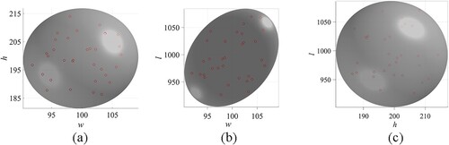
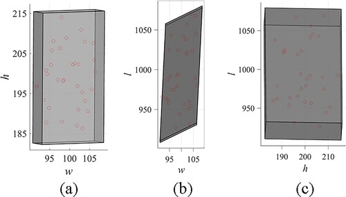
Figure 8. Projections of the MP model: (a) w-h plane; (b) w-l plane and (c) h-l plane.

Table 5 provides the key parameters of convex models established via different methods to facilitate a detailed comparison of various models. Herein, κ is the sample coverage rate, which is the ratio of samples included in the model to the total samples. From Table 5, we can observe that the centres of uncertainty domains represented by different models are approximate. In terms of modelling efficiency, the proposed method is faster than the CCC-based method and is similar to the SCC-based method. As for the sample coverage rate and volume of the convex models, the proposed method maintains a high sample coverage rate with a pleasurable volume size. In addition, we highlight that the proposed method has successfully removed the two edge data as erroneous data during modelling, while the other two methods overlook the erroneous samples. Therefore, we can conclude from this numerical example that the proposed method can construct convex models with superior comprehensive performance and efficiently provide accurate solutions.

Table 5. Key parameters of different convex models.

Type	Model	ζ	$\overline{\zeta }$	κ	t	X^m
Ellipsoid	Proposed	39.79%	73.55%	0.941	1.296	[99.79 199.11 993.91]
	CCC-based	39.72%	73.51%	0.844	1.632	[100 200 1000]
	SCC-based	41.23%	74.43%	0.853	1.177	[100 200 1000]
Parallelepiped	Proposed	45.42%	76.87%	0.941	1.297	[99.79 199.11 993.91]
	CCC-based	17.44%	55.87%	0.500	2.404	[100 200 1000]
	SCC-based	32.58%	68.81%	0.765	1.107	[100 200 1000]

4.3. LPBF-fabricated structures

4.3.1. Design and fabrication of the tested structures

Two types of representative structures, solid and lattice structures, are designed and fabricated using LPBF technology for tensile and compression experiments, as shown in Figure 9. The lattice structure used as the compression specimen is a triply periodic minimal surface (TPMS) porous structure composed of 4 × 4 × 4 unit cells with a size of 40 × 40 × 40 mm, which possess excellent compression and energy absorption effect due to its internal porous structure. The solid structure used as the tensile specimen is a standard specimen with a total length of 170 mm and a width of 10 mm. 316L stainless steel and AlSi10Mg aluminium alloy are utilised to fabricate the structures. The details about the chemical composition of the two raw materials used for printing are tested and shown in Table 6 and Table 7. The particle size distribution of spherical powders for both materials is 15 µm to 53 µm, with a median particle size of 32.7 µm for 316L material and 38 µm for AlSi10Mg material. The apparent density of 316L stainless steel spherical powder is 4.18 g/cm3 and the flowability defined by the Hall flowmeter is 18 s/50 g. And the apparent density of AlSi10Mg aluminium alloy spherical powder is 1.36 g/cm3 and the flowability is 65.8 s/50 g.

Figure 9. Two representative structures fabricated by LPBF: (a) Solid structure and (b) lattice structure.

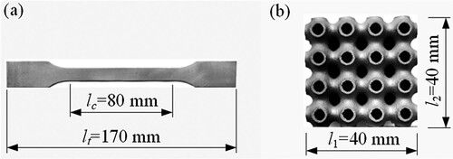
Table 6. The chemical composition of the 316L stainless steel powder.

Element	Fe	Cr	Ni	Mo	Mn	Si	P	C	S	O
Wt. %	Bal	17.31	11.31	2.66	1.51	0.62	0.01	0.011	0.007	0.056

Table 7. The chemical composition of the AlSi10Mg aluminium alloy powder.

Element	Al	Si	Mg	Fe	Cu	Mn	Ni	Zn	Ti
Wt. %	Bal	10.20	0.29	0.039	<0.01	<0.01	<0.01	<0.01	<0.01

The LPBF process is conducted on a DiMetal-100 SLM machine developed by the South China University of Technology. All the manufacturing processing occurs in a nitrogen environment where the O2 content is less than 0.05%, and the dust removal rate is greater than 95%. The detailed LPBF processing parameters used by the DiMetal-100 machine are summarised in Table 8. The printing direction of AM process is shown in Figure 10. The solid structure sample is printed vertically along the X direction, and the lattice structure sample is normally stacked and printed on the XY plane.

Figure 10. The building direction of the structure samples on the powder bed.

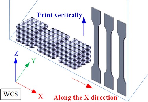
Table 8. The processing parameters used by the LPBF.

Devices	Material	Laser power	Scanning speed
DiMetal-100	316L	40 W	350 mm/s
DiMetal-100	AlSi10Mg	75 W	250 mm/s

4.3.2. Experiments for testing physical properties

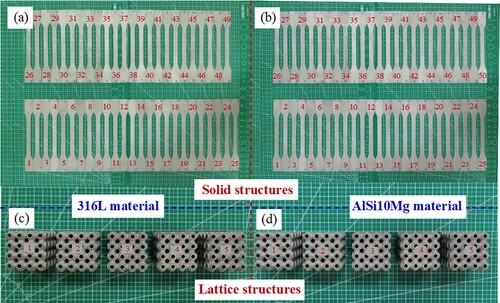
Figure 11 shows the printing results of two representative structures via LPBF. Figure 11(a) and Figure 11(b) are solid structure samples printed using 316L and AlSi10Mg materials, respectively; Figure 11(c) and Figure 11(d) are the lattice structure samples printed using 316L and AlSi10Mg material, respectively. Due to the LPBF involving a series of coupled physical phenomena, the process-structure–property relationship is extremely complex. The mechanical properties of the printed parts are directly determined by the microstructure, and also considerably affected by the residual stress. Therefore, the inherently uncertain performance of the LPBF-fabricated structures mainly stems from the microstructure and residual stress. The mechanical properties exhibited by the printed macro-scale structure directly reflect the comprehensive influence of the microstructure and residual stress. From this perspective, analyzing the uncertain mechanical properties of the macro-scale structure can verify the inherent uncertainty in the comprehensive performance of the LPBF-fabricated structure.

Figure 11. Specimens fabricated by LPBF for experiments: (a) 316L solid structures; (b) AlSi10Mg solid structures; (c) 316L lattice structures; (d) AlSi10Mg lattice structures.

Firstly, to confirm the uncertainty of LPBF-fabricated structures, the mass and density of the 50 solid samples with AlSi10Mg material are tested. It is found that the mass of the sample specimen is between 7.289 and 7.654 g, and the density is between 3.0618 and 3.2149 g/m3, qualitatively indicating that there are indeed significant uncertainties in LPBF-fabricated structures. Then, we measure the mechanical properties of the 316L specimens by conducting several experiments. During the experiments, the displacement change is read using an extensometer, and the force value is recorded by a universal testing machine. The stress–strain curve is calculated by comparing each determined displacement value and its corresponding force value in the experimental data. The load range applied in the tensile test is 0∼5540 N, while it is 0∼73456 N before the densification stage in the compression test. Figure 12 presents the final states of the LPBF-fabricated structures after performing the experiments, while Figure 13 gives the corresponding stress–strain curves. It can be found that there is not much difference in appearance among the structures manufactured by LPBF, but there are significant differences in mechanical properties. For example, in tensile tests, the fracture of solid structures is located at different positions, and there are certain differences in the stress–strain curves of each solid structure. To quantify the differences among LPBF-fabricated structures, we conduct comprehensive experiments on a total of 49 samples of the 316L solid structure to measure the density, weight, elastic modulus, yield strength, and tensile strength. Finally, 34 sets of effective data are obtained as shown in Table 9. The physical parameters of these structures obviously fluctuate within a certain range, which can significantly influence the engineering application of structures. Additionally, the physical parameters of the 5 lattice structure samples, including the density, weight, elastic modulus and compressive strength, also exhibit fluctuations as shown in Table 10. Therefore, accounting for uncertainties of structures manufactured by LPBF with limited data is of necessity and urgency.

Figure 12. Final states of the specimens fabricated by LPBF: (a) 316L solid structures in tensile tests; (b) 316L lattice structures in compression tests.

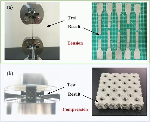
Figure 13. Stress-strain curves of specimens fabricated by LPBF: (a) 316L solid structures in tensile tests; (b) 316L lattice structures in compression tests.

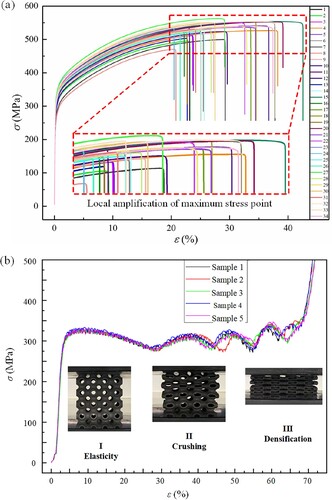
Table 9. Physical parameters of the 316L solid structures from tensile experiments.

No.	Elastic modulus (MPa)	Yield strength (MPa)	Tensile strength (MPa)	Weight (g)	Density (g/mm3)
1	167236	321	552	17.830	7.490
2	163997	290	495	17.808	7.480
3	159210	307	512	17.969	7.548
4	163621	298	527	18.016	7.568
5	165945	302	512	17.955	7.540
6	164524	305	516	17.793	7.474
7	168944	273	500	17.852	7.499
8	165624	265	470	17.815	7.483
9	169876	291	519	17.884	7.512
10	168487	318	541	18.064	7.588
11	171626	325	535	17.979	7.552
12	160124	305	524	17.939	7.535
13	162575	296	503	17.790	7.472
14	165010	323	533	17.836	7.492
15	165578	324	554	18.039	7.577
16	161851	316	521	17.790	7.472
17	166662	313	538	17.916	7.526
18	173871	323	554	17.834	7.491
19	168778	318	522	17.992	7.558
20	170184	321	552	18.515	7.777
21	171301	311	537	17.850	7.498
22	174322	321	551	17.935	7.534
23	170533	318	528	17.896	7.517
24	170728	330	534	17.844	7.495
25	163383	313	523	17.971	7.549
26	166512	316	518	17.947	7.539
27	171426	335	563	17.879	7.510
28	159103	316	529	17.992	7.557
29	172970	318	539	18.057	7.585
30	168006	320	550	17.789	7.472
31	168863	320	530	17.984	7.554
32	170965	324	554	17.820	7.485
33	172005	326	552	17.868	7.505
34	167048	316	540	17.978	7.552

Table 10. Physical parameters of the 316L lattice structures from compression experiments.

No.	Elastic modulus (GPa)	Compressive strength (MPa)	Weight (g)	Density (g/mm3)
1	17.0	327.4	108.772	8.09
2	17.3	329.1	109.353	8.13
3	17.0	326.4	109.176	8.13
4	17.3	333.6	109.513	8.14
5	17.2	329.7	109.316	8.13

4.3.3. Uncertainty quantification

Herein, in light of the experimental data related to the physical parameters of the 316L solid structures in Table 9, we can apply the proposed convex modelling method to quantify the structural uncertainties. By adopting the corresponding ellipsoid model, the uncertainties of parameters can be mathematically quantified as. (17) $\begin{array}{rl}& {\left[\begin{array}{c}(E-167379)/10014\\ ({\sigma }_S-312)/57\\ ({\sigma }_b-530)/73\\ (W-17.924)/0.715\\ (D-7.529)/0.300\end{array}\right]}^{\mathrm{T}}\\ & {\left[\begin{array}{ccccc}1& 0.3593& 0.5078& 0.0782& 0.0796\\ 0.3593& 1& 0.8596& 0.2096& 0.2100\\ 0.5078& 0.8596& 1& 0.2611& 0.2623\\ 0.0782& 0.2096& 0.2611& 1& 1.000\\ 0.0796& 0.2100& 0.2623& 1.000& 1\end{array}\right]}^{-1}\\ & \left[\begin{array}{c}(E-167379)/10014\\ ({\sigma }_S-312)/57\\ ({\sigma }_b-530)/73\\ (W-17.924)/0.715\\ (\rho -7.529)/0.300\end{array}\right]\le 1\end{array}$(17) where E, σS and σb are the elastic modulus, yield strength and tensile strength, respectively. W is the weight and D is the density. From the correlation matrix, it can be noted that the correlations between various parameters are different. Among them, the correlation between E and W is very small, only 0.0782, revealing that the two parameters correlate less. However, interestingly, the correlation between W and D is equal to 1, indicating a direct correlation between the two parameters, which is consistent with our common sense as density can be calculated by weight and proves the accuracy of the established convex model. To provide more intuitive information about uncertainties described in the model, Table 11 displays the corresponding variation intervals, centres, and radii for each parameter. Considering the importance of porosity formed by the microstructure in LPBF-fabricated structures, the ratio of density’s deviation to the median is used as an indicator to quantitatively evaluate the uncertainty. Thus, according to the uncertainty quantification results of the proposed method, the uncertainty indicator of the LPBF-fabricated solid structure can be marked as 3.98%.

Table 11. Variation intervals of physical parameters of LPBF-fabricated solid structures.

Physical parameter	Variation interval	Centre	Radius
Elastic modulus (MPa)	[157365, 177393]	167379	10014
Yield strength (MPa)	[255, 369]	312	57
Tensile strength (MPa)	[457, 603]	530	73
Weight (g)	[17.209, 18.639]	17.924	0.715
Density (g/mm3)	[7.229, 7.829]	7.529	0.300

Similarly, according to the sample data from the compression experiment of the LPBF-fabricated lattice structure in Table 10, the proposed method can be used to quantify the uncertainties. By adopting the proposed convex modelling method, the ellipsoid model for uncertainty quantification of parameters can be expressed as. (18) $\begin{array}{rl}& {\left[\begin{array}{c}(E-17.2)/0.2\\ ({\sigma }_C-330.0)/3.7\\ (W-109.239)/0.471\\ (D-8.12)/0.03\end{array}\right]}^{\mathrm{T}}\\ & {\left[\begin{array}{cccc}1& 0.7104& 0.9661& 0.9567\\ 0.7104& 1& 0.8181& 0.7944\\ 0.9661& 0.8181& 1& 0.9977\\ 0.6567& 0.7944& 0.9977& 1\end{array}\right]}^{-1}\\ & \left[\begin{array}{c}(E-17.2)/0.2\\ ({\sigma }_C-330.0)/3.7\\ (W-109.239)/0.471\\ (D-8.12)/0.03\end{array}\right]\le 1\end{array}$(18) where σC is the compressive strength. From the correlation matrix, it can be found that apart from the consistent correlation between W and D, the correlation between parameters of lattice structures is significantly different from that of solid structures. For example, the correlation between E and W reaches 0.9661, indicating a strong correlation between these two parameters. This completely different result from the solid structure is essentially caused by the internal microstructure of the lattice structure. Therefore, the established correlation matrix is reasonable. Table 12 shows the variation intervals, centres, and radii for each parameter. Correspondingly, the uncertainty indicator of the LPBF-fabricated lattice structure can be calculated as 0.37% based on the results of the proposed method. This is smaller than the uncertainty indicator of the solid structure, indicating that the fluctuation of its density is relatively stable, that is, the change in porosity is small.

Table 12. Variation intervals of physical parameters of LPBF-fabricated lattice structures.

Physical parameter	Variation interval	Centre	Radius
Elastic modulus (MPa)	[17.0, 17.4]	17.2	0.2
Compressive (MPa)	[326.3, 333.6]	330.0	3.69
Weight (g)	[108.767, 109.710]	109.239	0.471
Density (g/mm3)	[8.09, 8.16]	8.12	0.03

Combining Table 10 and Table 12, it can be seen that although the small amount of data from the compression test can have a certain impact on the result, it does not affect the good application of the model. Furthermore, it is worth noting that during the modelling process of structural compression test data using the proposed method, the fourth set of test data was automatically removed. If not removed, the uncertainty intervals of the obtained parameters are very large, such as $E^I=[14.1,20.2]$MPa, ${\sigma }_C^I=[245.1,413.4]$MPa, which is unreasonable and meaningless.

With the acquired information on the LPBF-fabricated solid structure and lattice structure, we have achieved measurement of various uncertain variables using the proposed method, further verifying the effectiveness of the uncertainty modelling framework proposed in this paper.

5. Conclusions

Owing to the complicated manufacturing process of LPBF-fabricated structures, the processing tolerance inevitably exists, and the sample data is limited, resulting in the difficulty of dealing with uncertainties. To efficiently and exactly quantify the uncertainties of structures fabricated by LPBF with limited data, we have proposed a non-probabilistic convex modelling framework. By applying the proposed framework, the constructed convex models can accurately enclose the sample points concerning uncertain parameters with high efficiency and superior cost performance. We have established critical criteria and comprehensively investigated the application performance of the proposed method via test standards and comparison. We conclude that the proposed non-probabilistic convex modelling framework not only offers new opportunities for applying convex models to LPBF-fabricated structures with limited data but also provides a deeper understanding of the characteristics of convex models that can be particularly important. The proposed strategy is promising to provide theoretical guidance for the precise characterisation of the properties of LPBF-fabricated high-performance structures. Of course, the proposed convex modelling method also has some limitations, such as the inability to display the probability distribution of variables due to being a convex model based on limited samples, and the acquired variable intervals may not be accurate due to the significant influence of the limited samples. In future work, we will improve our modelling methods and discuss the quantitative analysis of uncertainty in the fabricating process of structures from multiple dimensions, such as material properties, preparation process, measurement errors, and numerical solutions. We will specifically analyze and measure the hardness, roughness, and residual stress of the LPBF-fabricated structure to describe its integrity.

CRediT authorship contribution statement

G. Zhao: Writing-original draft, Conceptualisation, Formal analysis, Investigation, Methodology, Supervision. R. Wang: Conceptualisation, Investigation, Validation, Data curation. F. Li: Methodology, Investigation. J. Liu: Writing-review & editing, Funding acquisition, Project administration, Methodology, Supervision.

Acknowledgements

Thanks very much to the reviewers for their comments on the paper.

Data availability

Data available on request from the authors.

Disclosure statement

No potential conflict of interest was reported by the author(s).

Additional information

Funding

This work was supported by National Natural Science Foundation of China: [grant no 12172095]; Guangzhou Science and Technology Planning Project: [grant no 202201020193;202201010399]; Anhui Provincial Department of Education: [grant no KJ2021A0157].

References

- Liu J, Chen T, Zhang Y, et al. On sound insulation of pyramidal lattice sandwich structure. Compos Struct. 2019a;208:385–394. doi:10.1016/j.compstruct.2018.10.013.
- Liu J, Ou H, Zeng R, et al. Fabrication, dynamic properties and multi-objective optimization of a metal origami tube with Miura sheets. Thin-Walled Struct. 2019b;144:106352, doi:10.1016/j.tws.2019.106352.
- Zhang Y, Xu X, Fang J, et al. Load characteristics of triangular honeycomb structures with self-similar hierarchical features. Eng Struct. 2022;257:114114, doi:10.1016/j.engstruct.2022.114114.
- Liu H, Gu D, Qi J, et al. Dimensional effect and mechanical performance of node-strengthened hybrid lattice structure fabricated by laser powder bed fusion. Virtual Phys Prototyp. 2023;18(1), doi:10.1080/17452759.2023.2240306.
- Yin S, Chen H, Wu Y, et al. Introducing composite lattice core sandwich structure as an alternative proposal for engine hood. Compos Struct. 2018;201:131–140. doi:10.1016/j.compstruct.2018.06.038.
- Sha W, Xiao M, Zhang J, et al. Robustly printable freeform thermal metamaterials. Nat Commun. 2021;12(1):7228, doi:10.1038/s41467-021-27543-7.
- Chen B, Chen L, Du B, et al. Novel multifunctional negative stiffness mechanical metamaterial structure: tailored functions of multi-stable and compressive mono-stable. Composites Part B: Engineering. 2021;204:108501, doi:10.1016/j.compositesb.2020.108501.
- Blakey-Milner B, Gradl P, Snedden G, et al. Metal additive manufacturing in aerospace: a review. Mater Des. 2021;209:110008, doi:10.1016/j.matdes.2021.110008.
- Liu G, Zhang X, Chen X, et al. Additive manufacturing of structural materials. Materials Science and Engineering: R: Reports. 2021;145:100596.
- Kumar SP, Elangovan S, Mohanraj R, et al. Review on the evolution and technology of State-of-the-Art metal additive manufacturing processes. Mater Today Proc. 2021;46:7907–7920. doi:10.1016/j.matpr.2021.02.567.
- Yap CY, Chua CK, Dong ZL, et al. Review of selective laser melting: materials and applications. Appl Phys Rev. 2015;2(4):041101, doi:10.1063/1.4935926.
- Nagarajan B, Hu Z, Song X, et al. Development of micro selective laser melting: the state of the art and future perspectives. Engineering. 2019;5(4):702–720. doi:10.1016/j.eng.2019.07.002.
- Nagesha BK, Dhinakaran V, Varsha Shree M, et al. Review on characterization and impacts of the lattice structure in additive manufacturing. Mater Today Proc. 2020;21:916–919. doi:10.1016/j.matpr.2019.08.158.
- Gu D, Shi X, Poprawe R, et al. Material-structure-performance integrated laser-metal additive manufacturing. Science. 2021;372(6545):eabg1487, doi:10.1126/science.abg1487.
- Delcuse L, Bahi S, Gunputh U, et al. Effect of powder bed fusion laser melting process parameters, build orientation and strut thickness on porosity, accuracy and tensile properties of an auxetic structure in IN718 alloy. Addit Manuf. 2020;36:101339, doi:10.1016/j.addma.2020.101339.
- Meng L, Lan X, Zhao J, et al. Failure analysis of bio-inspired corrugated sandwich structures fabricated by laser powder bed fusion under three-point bending. Compos Struct. 2021;263:113724, doi:10.1016/j.compstruct.2021.113724.
- Zhong T, He K, Li H, et al. Mechanical properties of lightweight 316L stainless steel lattice structures fabricated by selective laser melting. Mater Des. 2019;181:108076, doi:10.1016/j.matdes.2019.108076.
- Dzugan J, Seifi M, Rzepa S, et al. Mechanical properties characterisation of metallic components produced by additive manufacturing using miniaturised specimens. Virtual Phys Prototyp. 2023;18(1):2161400, doi:10.1080/17452759.2022.2161400.
- Mukalay TA, Trimble JA, Mpofu K, et al. A systematic review of process uncertainty in Ti6Al4V-selective laser melting. CIRP J Manuf Sci Technol. 2022;36:185–212. doi:10.1016/j.cirpj.2021.12.005.
- Zocca A, Wilbig J, Waske A, et al. Challenges in the technology development for additive manufacturing in space. Chin J Mech Eng: Addit Manuf Front. 2022;1(1):100018, doi:10.1016/j.cjmeam.2022.100018.
- Moser D, Cullinan M, Murthy J. Multi-scale computational modeling of residual stress in selective laser melting with uncertainty quantification. Addit Manuf. 2019;29:100770, doi:10.1016/j.addma.2019.06.021.
- Chen Z, Han C, Gao M, et al. A review on qualification and certification for metal additive manufacturing. Virtual Phys Prototyp. 2022;17(2):382–405. doi:10.1080/17452759.2021.2018938.
- Lin Q, Hu J, Zhou Q, et al. Multi-output Gaussian process prediction for computationally expensive problems with multiple levels of fidelity. Knowl Based Syst. 2021;227:107151, doi:10.1016/j.knosys.2021.107151.
- Cao L, Liu J, Xie L, et al. Non-probabilistic polygonal convex set model for structural uncertainty quantification. Appl Math Model. 2021;89:504–518. doi:10.1016/j.apm.2020.07.025.
- Wang L, Liu Y, Li M. Time-dependent reliability-based optimization for structural-topological configuration design under convex-bounded uncertain modeling. Reliab Eng Syst Saf. 2022;221:108361, doi:10.1016/j.ress.2022.108361.
- Kang Z, Zhang W. Construction and application of an ellipsoidal convex model using a semi-definite programming formulation from measured data. Comput Methods Appl Mech Eng. 2016;300:461–489. doi:10.1016/j.cma.2015.11.025.
- Zhao MY, Yan WJ, Veng Yuen K, et al. Non-probabilistic uncertainty quantification for dynamic characterization functions using complex ratio interval arithmetic operation of multidimensional parallelepiped model. Mech Syst Signal Process. 2021;156:107559, doi:10.1016/j.ymssp.2020.107559.
- Jiang C, Han X, Lu GY, et al. Correlation analysis of non-probabilistic convex model and corresponding structural reliability technique. Comput Methods Appl Mech Eng. 2011;200(33-36):2528–2546. doi:10.1016/j.cma.2011.04.007.
- Xu M, Du J, Wang C, et al. A dual-layer dimension-wise fuzzy finite element method for structural analysis with epistemic uncertainties. Fuzzy Sets Syst. 2019;367:68–81. doi:10.1016/j.fss.2018.08.010.
- Luo Y, Zhan J, Xing J, et al. Non-probabilistic uncertainty quantification and response analysis of structures with a bounded field model. Comput Methods Appl Mech Eng. 2019;347:663–678. doi:10.1016/j.cma.2018.12.043.
- Zhao G, Liu J, Wen G, et al. Non-probabilistic convex model theory to obtain failure shear stress of simulated lunar soil under interval uncertainties. Probab Eng Mech. 2018;53:87–94. doi:10.1016/j.probengmech.2018.06.002.
- Zhao G, Wen G, Liu J. A novel analysis method for vibration systems under time-varying uncertainties based on interval process model. Probab Eng Mech. 2022;70:103363, doi:10.1016/j.probengmech.2022.103363.
- Gorguluarslan RM, Choi S-K, Saldana CJ. Uncertainty quantification and validation of 3D lattice scaffolds for computer-aided biomedical applications. J Mech Behav Biomed Mater. 2017;71:428–440. doi:10.1016/j.jmbbm.2017.04.011.
- Li F, Wang R, Zheng Z, et al. A time-variant reliability analysis framework for selective laser melting fabricated lattice structures with probability and convex hybrid models. Virtual Phys Prototyp. 2022;17(4):841–853. doi:10.1080/17452759.2022.2074196.
- Lozanovski B, Downing D, Tran P, et al. A Monte Carlo simulation-based approach to realistic modelling of additively manufactured lattice structures. Addit Manuf. 2020;32:101092, doi:10.1016/j.addma.2020.101092.
- Snider-Simon B, Frantziskonis G. Reliability of metal additive manufactured materials from modeling the microstructure at different length scales. Addit Manuf. 2022;51:102629, doi:10.1016/j.addma.2022.102629.
- Zhao G, Liu J, Wen G, et al. A novel method for non-probabilistic convex modelling based on data from practical engineering. Appl Math Model. 2020;80:516–530. doi:10.1016/j.apm.2019.12.002.
- Cui Y, Geng Z, Zhu Q, et al. Review: multi-objective optimization methods and application in energy saving. Energy. 2017;125:681–704. doi:10.1016/j.energy.2017.02.174.
- Ni BY, Jiang C, Huang ZL. Discussions on non-probabilistic convex modelling for uncertain problems. Appl Math Model. 2018;59:54–85. doi:10.1016/j.apm.2018.01.026.
- Shen C, Bao X, Tan J, et al. Two noise-robust axial scanning multi-image phase retrieval algorithms based on Pauta criterion and smoothness constraint. Opt Express. 2017;25(14):16235–16249. doi:10.1364/OE.25.016235.
- Jiang C, Bi RG, Lu GY, et al. Structural reliability analysis using non-probabilistic convex model. Comput Methods Appl Mech Eng. 2013;254:83–98. doi:10.1016/j.cma.2012.10.020.