
 ?Mathematical formulae have been encoded as MathML and are displayed in this HTML version using MathJax in order to improve their display. Uncheck the box to turn MathJax off. This feature requires Javascript. Click on a formula to zoom.
ABSTRACT
Curved layering has become one of the current research hotspots for its unique advantages. In order to improve the adaptability and accuracy, this paper proposes a new curved layering and path planning algorithm based on voxelization and geodesic distance. High density discrete points are used to approximate the shortest path, voxelization and new optimized search algorithm are adopted to obtain the geodesic distance field within stereolithography (STL) model. Curved layers are formed from points with equal geodesic distance values. The developed algorithm overcomes the limitations of the existing facet offsetting method. Moreover, robot positioner angle planning strategies are exploited to achieve good formation for support-free curved layers of spatial overhang characteristics. The results of comparative analysis and verification experiment indicate that the algorithm accuracy is not affected by the size and intersection angle of the triangles, satisfies the high-precision requirements for parts with curved surface in robotic GMA additive manufacturing.
1. Introduction
Additive manufacturing (AM) is a layer-by-layer manufacturing technology. Compared with traditional casting, forging and other manufacturing methods, it has the advantages of no mold, short processing cycle and high material utilization. AM has been used in aviation, aerospace, vehicles and other fields [Citation1–3]. Gas metal arc (GMA) additive manufacturing is a type of metal additive manufacturing which has been widely researched due to its merits of high deposition efficiency and low equipment cost in comparison with laser AM, electron beam AM and other metal additive manufacturing methods [Citation4,Citation5].
1.1. The advantages of curved layering algorithm
At present, the contradiction between forming accuracy and efficiency is one of the main problems that needs to be solved in AM field. Achieving high-precision and high-efficiency additive manufacturing is the research goal [Citation6]. Slicing algorithm is a widely concerned solution [Citation7,Citation8]. For the complex parts with large curvature surface, the traditional planar layering will cause the staircase effect as shown in (a). The staircase effect increases the roughness of the part surface and seriously affects the forming accuracy [Citation9].
Figure 1. Staircase effect. (a) Planar layering, (b) adaptive layering and (c) curved layering.
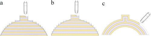
The conventional method to reduce the staircase effect is to reduce the layer thickness. The adaptive layering algorithms have been proposed [Citation10,Citation11], as shown in (b). The thickness of the layers is changed according to the model surface curvature. As the layer thickness decreases, the impact of the step effect diminishes. However, due to process constraints, layer thickness cannot be reduced infinitely. Simultaneously, decreasing the layer thickness increases the total number of layers, thereby extending manufacturing time [Citation12]. In order to alleviate the staircase effect, the idea of curved layering was proposed [Citation13], which broke the pattern of planar slicing and used a set of spatial curved surfaces instead of planes to slice the three-dimensional model of parts, as shown in (c).
Curved layering has the following advantages in contrast to planar slicing [Citation14–16]:
The staircase effect on the surface is alleviated and the forming quality is better.
The number of deposited layers is fewer, the length of the deposited paths is longer, and the deposition efficiency is higher.
There are fewer arc starting points and arc extinction points, and the forming quality is better.
The unique advantages make curved layering more suitable for parts with inclined surfaces or large curvature surfaces. As a result, the curved layering method has gradually become a research hotspot.
1.2. The development of curved layering algorithm and path planning algorithm on spatial surfaces
Curved layering was first proposed in the field of fused deposition modeling (FDM) and is called curved layered fused deposition modeling (CLFDM) [Citation17]. According to the literature, algorithms are divided into two categories: characteristic equation-based and STL model-based.
In characteristic equation-based algorithm, the B-spline curve equation was used to identify the key points on the curved surface. Through optimization by genetic algorithms, normal surface offsetting and surface–surface intersection, adaptive curved layering with key surface features could be retained [Citation18]. NURBS equation was also adopted to describe curved surfaces, dividing complex curved surfaces into a certain number of simple sub-regions. Different sub-regions were deposited in different postures to achieve a uniform thickness layer on the curved surface using wire and arc additive manufacturing (WAAM), but the additive manufacturing of typical parts was not realised [Citation19]. The cross-section profile was obtained by the intersection operation of the cylinder equation and blade, and a propeller based on cylindrical layering was fabricated [Citation20]. The blades of underwater thruster were also fabricated on conical surface using a parametric slicing equation [Citation21]. On the whole, although the characteristic equation-based algorithms for curved layering are relatively simple, the algorithms have narrow adaptability.
In additive manufacturing, the mainstream model file format is STL, and some curved layering algorithms based on STL have been developed. An algorithm to achieve curved layering by facet offsetting along the normal direction was proposed [Citation22]. The points on the translated surface were obtained by intersecting three planes. The algorithm accuracy was poor when the angle between adjacent triangular pieces changed drastically.
Furthermore, through a surface embedded field, whose value at any particular point was the geodesic distance to the specified bottom of the model, curved layering could be achieved [Citation23]. However, the Mitchell Mount Papadimitriou (MMP) method could only obtain the distance field on the surfaces of the parts, rather than the internal distance field. This method could not guarantee the uniform thickness of the internal layer. The filling amount needs to be adjusted in real time which was very difficult to implement.
The method based on geodesic distance is a promising tool to construct curved layer. A curved layering method using isothermal surface through heat transfer simulation was proposed [Citation24]. Parts were virtually placed on a heated substrate to establish a temperature field, and the isothermal surface naturally generated a curved layer. This method was used in FDM, and its versatility was poor. The geodesic distance could also be constructed by mesh interpolation using the thermal diffusion method [Citation25] to realise five-axis linkage machining of complex free-form surface solid parts. However, this interpolation method cannot guarantee the accuracy of geodesic distance.
On the other hand, curved layering also introduces new challenges in the path planning for spatial surfaces. In comparison to path planning in planar layer, the spacing of paths on spatial surfaces must be carefully controlled to ensure the quality of the cladding layer [Citation26]. A tangent plane was constructed at a point along the known path on the surface, and points adjacent to this path could be determined based on the cross-sectional shape of the FDM filament and the section of the surface [Citation27]. However, it should be noted that this algorithm approximates each section between adjacent paths as a plane, which may not be suitable for GMA additive manufacturing process with large beam widths. By flattening the curved surface, the paths could be generated on flattened plane, then reversely transformed to the curved layer [Citation7]. This method demanded the curved surface should be developable, but not all surfaces meet this condition. Considering the difficulty of self-developing path planning algorithm, a commercial 3D modeling software such as Rhinoceros® has been redeveloped [Citation28]. It could also realise curved layering and path planning on curved surfaces, and the advantages of curved layering compared to planar layering in surface quality, printing time, and surface strength were verified through the 3D concrete printing test.
To sum up, the curved layering algorithm has relatively mature developed in the FDM field, and there have been reports of the related curved layering devices [Citation29]. However, it is still in the embryonic and preliminary exploration stage for metal additive manufacturing, and there are many challenges. This paper is dedicated to developing a universal equal-thickness curved layering and surface equidistant path planning algorithm suitable for the STL file format. Voxelization and optimised search methods are used to calculate the space geodesic distance field, and a new layered surface is formed from discrete points with equal geodesic distance value. In addition, a welding torch posture planning strategy is designed to ensure the good formation of the support-free curved layering with spatial overhang characteristics for robotic GMA-AM. These efforts ensure precise forming of additive manufacturing for complex curved parts, and will promote the application of curved layering in GMA-AM.
2. Curved layering algorithm based on voxelization
Considering GMA-AM process characteristics, this paper aims to obtain deposited layers of equal thickness. The steps of the proposed curved layering algorithm include: (1) Voxel representation of the closed model; (2) Calculation of the voxel points’ geodesic distance; (3) Construction of curved layered surface. This algorithm can achieve equal-thickness curved layering on any STL model. shows the layering results of the algorithm on logarithmic spiral gear, submarine shell and voxelization. The implementation details of the algorithm are given below.
2.1. Voxelization representation and storage structure design
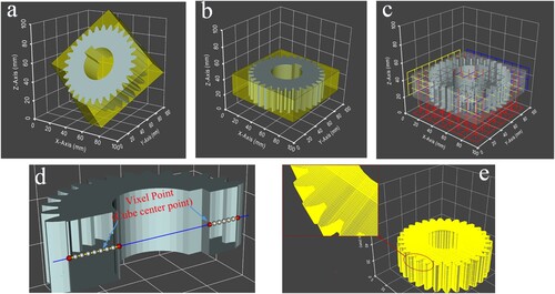
Voxelization refers to the method of using a group of tiny cubes in space to represent the model. The procedure of voxelization is shown in . Firstly, Principal Component Analysis (PCA) method is used to analyze the geometric features of the STL model in order to obtain the minimum bounding box, as shown in (a). The length, width, and height directions of the bounding box are rotated to the X, Y and Z-axis direction of the global coordinate system respectively, as shown in (b). The bounding box is uniformly decomposed into numerous cubes through line segment cluster which parallel to the coordinate axis, as shown in (c). Each cube represents a voxel and its coordinate is denoted by position of the cube center. Intersection points between every line segment above mentioned and the model surface are calculated to obtain the part of the line segment that belongs to the interior of the model. The cubes passing through this part of the line segment are called effective voxel points, as shown in (d). The typical part voxelization result is illustrated in (e).
Figure 2. Layering results of typical parts based on voxelization. (a) Logarithmic spiral gear model, (b) submarine shell model, (c) pipe model, (d) logarithmic spiral gear layering result, (e) submarine shell layering result and (f) pipe layering result.
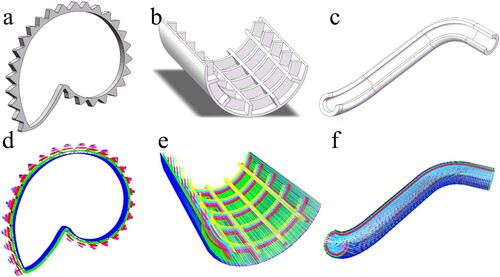
Figure 3. Voxelization procedure. (a) The minimum bounding box of the STL model, (b) model rotating, (c) meshing, (d) calculation of intersection point and (e) voxelization result.
The PCA method is used to reduce the projected area of the model on principal planes of the coordinate, thereby reducing the number of line segments that need to be calculated. But this does not really mean changing the direction of the model. After voxelization, the model will be rotated back to its original position for layering and path planning.
The higher the voxelization density, the better the fitting effect and algorithm accuracy; however, this also leads to increase time and space complexity. In curved layering and path planning algorithms, numerous neighbourhood search operations are required. It is necessary to design a storage structure with efficient query and calculation performance. This paper proposes a number-based red-black tree storage method. During voxelization, according to the coordinate, each voxel point is assigned a unique integer number as the red-black tree key. This approach effectively associates voxel point coordinate with an integer number, thereby optimising storage space utilization rate and computational efficiency. If the bounding box has dimensions l (length), w (width), and h (height), the voxel cube edge length is L, and the corresponding integer number N can be calculated for voxel P (Px, Py, Pz) as follows:
(1)
(1) The integer number N corresponds to the voxel point one by one, and the proof is as follows:
If there are two voxel points P1(Px1, Py1, Pz1) and P2(Px2, Py2, Pz2) with different coordinates and the same integer number, then there is
(2)
(2) Sort out:
(3)
(3)
(4)
(4) Since the coordinates of the voxel points are integer multiples of the side length L, we can get:
(5)
(5) Similarly, it can be inferred that:
(6)
(6)
(7)
(7) This is contrary to the hypothesis that P1 and P2 are two different voxel points, and the original proposition is proved.
In this way, with the help of formula (1), the coordinates of adjacent voxel points can be found based on its integer number, thus neighbourhood search operation is achieved. The search complexity of the red-black tree is only O(logV), while the kd-tree data structure is affected by many factors and may reach O(V) under unideal circumstances, where V is the number of voxel points. Therefore, through red-black tree storage, computing efficiency can be effectively improved, especially when the point cloud is huge, this advantage will be more obvious.
The test was carried out in a 1M voxel point set, using the kd-tree data structure to store the three-dimensional coordinates of voxel points and the red-black tree to store the integer number. 100k neighbourhood search operations were performed on the same computer and the operation time was recorded in . Compared with the kd-tree storage structure, the red-black tree storage structure can improve the neighbourhood search operation speed by about 70%.
Table 1. Comparison of neighbourhood search operation time with different data structure.
2.2. Geodesic distance calculation
2.2.1. The definitions of GDTC and GDTS
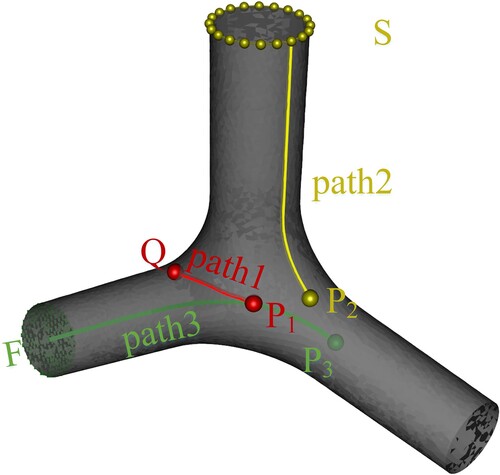
The premise of curved layering is to obtain the geodesic distance of all voxel points. Unlike Euclidean distance, geodesic distance is commonly used to describe the shortest path length between two points on a space curved surface. This paper extends the concept of ‘geodesic distance’, it also includes distances from point to curve and point to surface. The geodesic distance of point to curve refers to length of the shortest path from point to curve on the curved surface, recorded as GDTC. Similarly, the geodesic distance of point to surface refers to length of the shortest path from point to surface in the model, recorded as GDTS. As shown in , path1, path2 and path3 represent respectively the shortest paths between points, between point to curve, and between point to surface, their lengths correspondingly represent their values.
Figure 4. Extended geodesic distance diagram.
2.2.2. The calculation process of GDTS
The key of geodesic distance calculation is to find the shortest path from this point to another point, a curve or a surface. In graph theory, traversal method and Dijkstra algorithm are usually used to find the shortest path between two vertices on a graph. These methods are not suitable for graphs composed of a large number of voxel points.
For this reason, the method of geodesic distance calculation based on voxelization and optimized search is proposed in this paper. The voxel points on the initial curved layer given by users are defined as the initial source points and its geodesic distance is set at 0. Starting from the source points, the geodesic distances of surrounding voxel points are continuously calculated until the GDTS of all voxel points have been obtained. The specific steps of the algorithm are shown in :
| (1) | The voxel points on the initial curved layer are defined as the initial source points denoted by the reference point set B and their GDTS values are set at 0. During calculation of geodesic distance, set B is used for neighbourhood search operations. | ||||
| (2) | Categorise all voxel points into three groups: those with known GDTS values, their surrounding points with unknown GDTS values recorded as point set A, and other distant points. | ||||
| (3) | The GDTS value of voxel points in points set A are calculated. To compute the GDTS value of a voxel point, we must firstly search the shortest path from the voxel point to the curved surface. When the voxelization density is sufficiently high, this shortest path can be approximated by line segments through connecting voxel points, following the principle of integral. The GDTS value is represented as the sum of lengths along these line segments formed between adjacent voxel points on this path. illustrates the spatial neighbourhood search diagram for voxel points. In order to calculate the GDTS value of a specific voxel point P, it is necessary to consider P as the center, the red point in , and count neighbouring voxels (set N) in point set B. The formula for calculating the GDTS value of point P can be obtained as follows:
It should be noted that the point P and point set N are directly adjacent in space, and the straight line between two adjacent voxel points must be inside the model, so | ||||
| (4) | The maximum GDTS value in point set A is denoted as Smax, and reference point set B is updated with point set A. | ||||
| (5) | The point set to be calculated is divided into two parts according to whether the GDTS value is greater than | ||||
| (6) | Check whether C is an empty set. If yes, go to step 9. If no, go to step 7. | ||||
| (7) | Surrounding points of set C with unknown GDTS values are recorded as point set E, then calculate their geodesic distances by the method in step 3. | ||||
| (8) | Update reference point set B with the union of point sets D and E. Return to step 5. | ||||
| (9) | Determine if the GDTS values of all voxel points have been calculated. If yes, stop calculation and exit loop; if no, return to step 2. Figure 5. Flow chart of geodesic distance calculation. 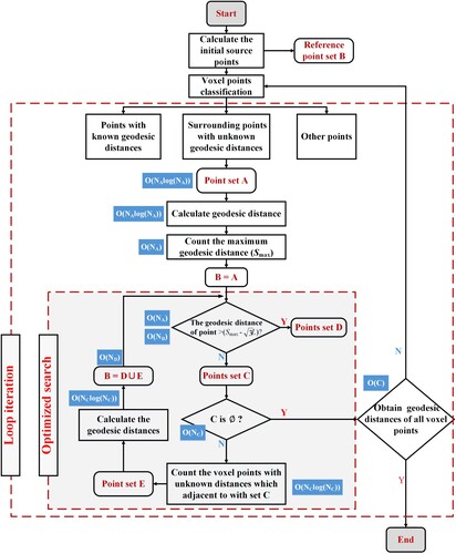 Figure 6. Schematic diagram of voxel point neighbourhood search. 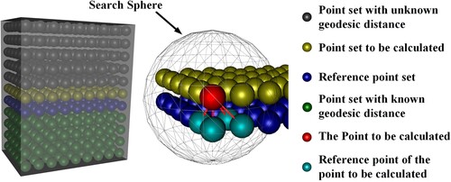 | ||||
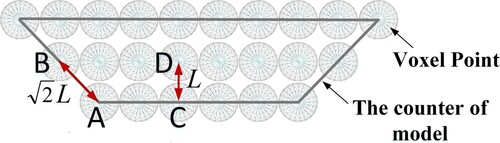
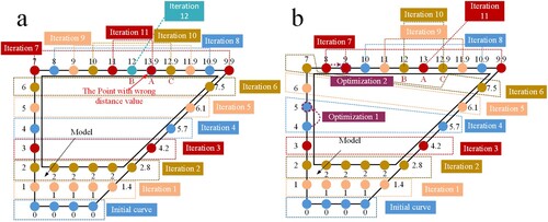
The purpose of steps 5–8 in the above algorithm is to correct GDTS value to ensure that the GDTS value distribution of all points in the reference point set is within the range of , which is a prerequisite to the correctness of the algorithm. As shown in , voxel points A and B, C and D are adjacent voxel points in the model. Through one iterative loop, the geodesic distances of point B increase
L and the one of point D increase L. This is not as expected, and the correction is obtained through algorithm steps 5–8.
Figure 7. Diagram of geodesic distance deviation.
2.2.3. Algorithm validity proof
GDTS value of every reference point in set B has a value range [,
], which is a key premise to ensure algorithm correctness. The proof process is as follows, shown in .
Figure 8. Diagram of proof process.
To prove that the GDTS value of voxel point P is correct, it is only necessary to prove that the shortest path from P to the initial surface must pass through a point in the search sphere. In other words, the GDTS value of point P obtained through point Q must be smaller than that obtained through point V:
(9)
(9) In ,
、
represent the GDTS values of voxel points V and Q respectively;
、
are expressed as the Euclidean distance between P and voxel points V and Q.
It can be obtained from formula (9):
(10)
(10) Because the GDTS values distribution of the reference point set must be within the range of
, it is only needed to prove:
(11)
(11) And
value equals the length of PQ, namely
, and Point V is outside of the search sphere, so the
> r. It can be obtained:
(12)
(12) If the radius of the search sphere is set to r = 2
L, the formula (9) can be verified, so that the GDTS value of point P can be obtained correctly.
2.2.4. Analysis of algorithm complexity and the significance of optimization search
The essence of GDTS value calculation is to find the shortest path within the model, which is a classic ‘Multiple-Source Shortest Path in Weighted Graph’ problem in graph theory. It is generally implemented through the Johnson algorithm, and the complexity is , where V is equivalent to the number of voxel points, and E is equivalent to the number of edges between voxel points. This paper effectively reduces the complexity to
by designing a number-based voxel point storage structure and optimized search, and improves the applicability of the shortest path search algorithm through voxelization.
The specific complexity of each step of the algorithm is marked in . Although the overall process of the algorithm is complex and contains two levels of loops. In general, the main calculation steps can be divided into three types: searching for the point set to be calculated, calculating the GDTS values of the points, and classifying voxel points. is a schematic diagram of the iterative calculation of GDTS value on a two-dimensional plane. (a) and (b) are divided into comparisons between direct search and optimization search. The propagation process that no matter whether optimization search is added or not, only one neighbourhood search and GDTS value calculation are needed for each voxel point. The complexity of searching once from the red-black tree is only , and GDTS value calculation for a fixed number of points only requires a constant number of operations. At the same time, it can be proved that the number of optimized search loop is at most 2 within an iteration, which means that the number of classifications must be less than 3 for a voxel point, so the complexity of classifying all voxel points is
. To sum up, the complexity of the algorithm is
.
Figure 9. Schematic diagram of geodetic distance calculation process. (a) Calculation process of direct search and (b) calculation process of optimization search.
This paper used the uniform distribution and continuous characteristics of voxel points, and proposed an optimization search strategy to ensure correctness without spending additional calculations. (b) illustrates that optimizing the search process can expedite the propagation along the shorter side. This ensures that point A is initially accessed through the shorter side, facilitating the acquisition of the correct GDTS value.
2.3. Construction of curved layered surface
If the shortest distance between any point on the surface Sa and the surface Sb is equal, then Sa is defined as the isometric surface of Sb. In order to obtain the equal thickness curved cladding layer, it requires the adjacent curved surfaces should be the isometric surfaces.
After the GDTS values of all voxel points are obtained, since the GDTS values are not continuous, the voxel points constructing curved surfaces for layering can be obtained according to formula (13):
(13)
(13)
is the set of points forming the ith layered surface, and it is easy to prove that the two adjacent layers obtained by this method meet the definition of isometric surfaces.
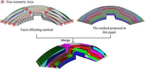
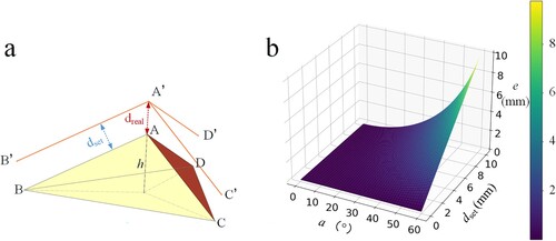
shows layering effects by facet offsetting method proposed in reference [Citation22] and the method proposed in this paper respectively. It can be seen that the isometric surfaces constructed by facet offsetting method are not strictly isometric.
Figure 10. Comparative effects of different curved layering methods.
The accuracy of the facet offsetting method is directly influenced by factors such as the size, intersection angle of the triangles, etc. In (a), point A is the common vertex of three congruent triangles, and O is the center of . The angle between vector
and
is denoted as α. Through simple geometric relationships, it can be deduced that the error in generating A’ after translation is:
(14)
(14)
is the desired offset distance, and
is the real offset distance of Point A. It can be seen from the error distribution in (b) that the facet offsetting algorithm error increases significantly with the increase of translation distance and triangle angle, and is not stable. The layered surface obtained by the method in this paper is the isometric surface of the previous layer, and the accuracy is less than or equal to the voxelization density, making it controllable. It is independent of uncontrollable random factors such as the size, intersection angle of the triangles, etc.
Figure 11. Error analysis of the facet offsetting method in degenerate case. (a) Schematic diagram of degradation situation and (b) error distribution.
3. Curved surface path planning and robot positioner angle planning
3.1. Curved surface path planning
In order to achieve a smooth cladding layer, for the GMA-AM process, it is necessary to keep the deposition beam spacing constant. Many detailed studies have been carried out. Theoretical overlap models such as Flat-top Overlapping Model [Citation30] and Tangent Overlapping Model [Citation31] were proposed. These models all aim at the overlap of deposition beams on the plane. Due to the different curvature of each point on the curved surface, the real deposition beam spacing on curved surface is not constant, will change with curvature. The deposition layers with good overlap cannot be obtained, as shown in .
Figure 12. The problem of traditional path planning.
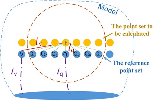
In this paper, according to the geodesic distance between the point to curve on the surface, the equidistant path planning on the curved surface consisted of voxel points is realised, and the good overlapping effect of adjacent deposition beams on the curved surface is obtained. The calculation method of GDTC value on the surface is the same as the one in section 2.2.
The difference is that the initial path is determined by intersection operation of an user-input surface and the STL model, and the voxel cubes passing through the initial path are taken as source points. In addition, the GDTC value l between two adjacent voxels cannot be directly replaced by the Euclidean distance, should be expressed by its projected length on the curved surface. The revised calculation formula is as follows:
(15)
(15) where
is the vector from Q to P,
is the normal direction of the surface at the voxel point P, and l is the projection length of the two points P and Q on the surface. The normal directions of voxel points on the surface can be calculated through point cloud filtering, tangent plane fitting and other algorithms.
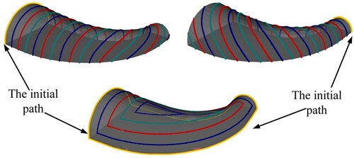
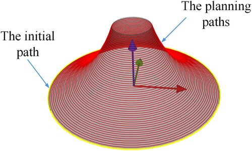
The points with the same GDTC values equal to the given beam spacing constitute the planned path. Since the voxel points are disordered and discrete, the robot deposition path cannot be directly output. Piecewise polynomial is used to fit path curves. When different initial path is set, the corresponding different path planning results will be obtained, as shown in . In other words, this method can achieve different types of planning paths by changing the initial paths.
Figure 13. Planning effects from different initial paths.
3.2. Robot positioner angle planning
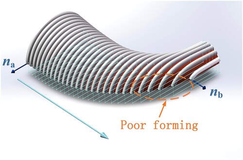
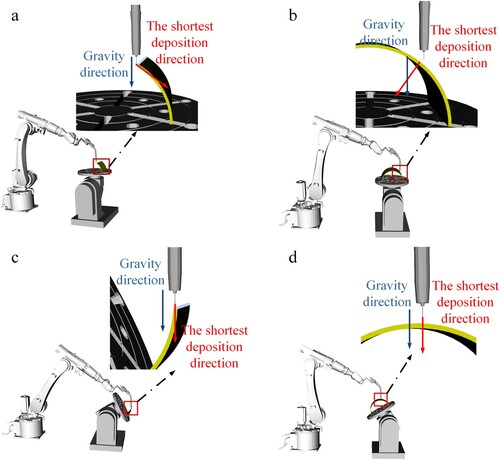
In planar layered additive manufacturing, the attitude of the welding torch is generally set perpendicular to the deposition layer, however, this strategy is not suitable for curved layer. In the process of GMA-AM, the molten pool on the spatial surface is dragged by gravity, and the deposition beam often presents an asymmetric cross-section, and it is difficult to obtain a well-formed deposition beam directly. In this paper, the arc is kept in vertical state, the spatial position of the surface is changed by the tilting positioner, and the forming effect of deposition beam depends on the angle planning of the tilting positioner. The vector from wire tip to the closest point on the deposited area is defined as the shortest deposition direction. The target of planning the joint angle of the tilting positioner is to keep the shortest deposition direction at gravity direction. In this condition the beam shaping is good.
The calculation of the shortest deposition direction is divided into two cases. When the first curved surface layer has not been deposited, the shortest deposition direction is directed from the wire tip to the nearest point in the former deposited beam, as shown in (a). When depositing the second and beyond curved layers, the shortest deposition direction is directed from the wire tip to the closest point in the previous deposited layer, as shown in (b). (c) and (d) are the schematic diagrams of adjusting the shortest deposition direction to the gravity direction through the motion of the tilting positioner.
Figure 14. Diagram of the shortest deposition direction and positioner angle planning. (a) The shortest deposition direction in case 1, (b) the shortest deposition direction in case 2, (c) adjust the shortest deposition direction in case 1 and (d) adjust the shortest deposition direction in case 2.
The steps and formulas for calculating the joint angle of the tilting positioner are described below. As shown in , arrows represent the shortest deposition direction in space. Firstly, through the rotation axis turning, the shortest deposition direction is perpendicular to the tilt axis, as shown in (b). Subsequently, through the movement of the tilt axis, the shortest deposition direction can be adjusted to vertical downward, as shown in (c).
Figure 15. Steps for calculating the joint angle of the positioner. (a) The shortest deposition direction at the initial position; (b) rotating movement and (c) tilting movement.
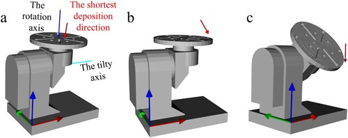
Assuming that the turning angle of the tilt axis is a1 and the turning angle of the rotation axis is a2, the following equations can be obtained:
(16)
(16) where
represents the shortest deposition direction,
represents the gravity vector,
,
are tilt axis, the rotation axis vector respectively, and
,
are the rotation matrixes when turning angles of a1, a2 around tilt axis and rotation axis respectively. For each point on the planning path, it is possible to calculate a set of joint angles according to formula (16) that keep the deposition process in the flat welding.
4. Verification experiment
In this paper, a turbine is selected as a typical component to verify the proposed algorithms of curved layering, path planning and joint angle planning of tilting positioner.
4.1. Experiment setup
The used GMA-AM system is shown in the (a). The motion mechanism includes a Motoman six-axis welding robot (HP20D) and a matching tilting positioner. A 1.2 mm diameter H08Mn2Si welding wire was used as the filling material and a Q235B steel plate was used as the test substrate, and their main chemical constituents s are shown in . The protective gas was a 5% CO2 + 95% Ar mixture. The algorithms proposed in this paper were developed using C++ language based on the offline programming software developed in our laboratory. The software uses the QT graphical interface library and the Visualization Toolkit (VTK) graphics library.
Figure 16. GMA-AM experiment setup. (a) Hardware and (b) software interface.
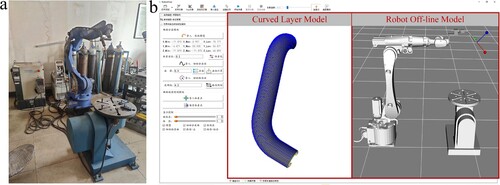
Table 2. Chemical constituents of substrate and wires (wt. %).
The selected verification turbine part is generally composed of a base and blades as shown in . At present, turbine manufacturing is mainly processed by multi-axis CNC machine. Due to the complex three-dimensional shape of the blade, the machined part is easy to interfere with the tool, and the generation of milling processing path is difficult. Alternatively, additive manufacturing provides a new processing method for turbine.
Figure 17. Feature dimensions and model of turbine. (a) Feature dimensions and (b) 3D-model.
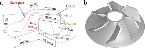
The base surface of the turbine is obtained by rotating a spline curve. The radius of the upper end is 50 mm, the radius of the lower end is 100 mm, the height is 55 mm, and the thickness of the blade is 10 mm. The torsion angle of the blade is 38°.
4.2. Curved layering and path planning of the turbine
Since the base surface is a spline surface, it also needs to be obtained through additive manufacturing. The turbine base was deposited on a 300*300 mm Q235 steel plate, the lower end of the base was selected as the initial path, and equidistant curve path planning was carried out on the surface of the turbine base, as shown in . Layer thickness here was set at 1.65 mm, and 54 deposition paths were obtained.
Figure 18. Path planning on turbine base surface.
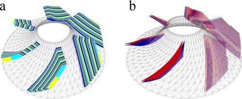
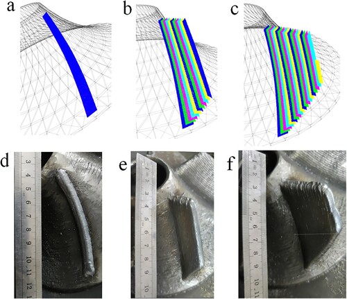
The turbine base outer surface is selected as the initial curved surface. For turbine blades, the layer thickness was set to 1.5 mm. The corresponding deposition speed was 7.0 mm/s, the width of the deposition beam was 5.9 mm, and the beam spacing was 3.7 mm. A total of 20 equidistant slicing curved surfaces were obtained by the above developed curved layering algorithm, as shown in (a). The edge of each curved layer of blade was selected as the initial path, and an equidistant parallel path was obtained by the above developed path planning algorithm, as shown in (b).
Figure 19. Curved layering and path planning of turbine blade. (a) Curved layering result and (b) path planning result.
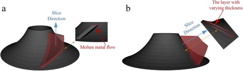
The effect of using planar layering method to slice the blade model is shown in . If slicing along the axial direction of the blade, the support between layers will be poor and molten metal flow will occur easily, as shown in (a). If slicing along the normal direction of substrate, the first layer obtained requires variable deposition thickness as shown in (b), which can cause accumulation of errors between layers and leading to forming defects easily.
Figure 20. The results of planar layering method. (a) Slicing along the axial direction of the blade and (b) slicing along the normal direction of substrate.
According to the positioner angle planning algorithm proposed in Section 3.2, the positioner joint angle values were calculated for each path point, and robot execution program is formed. and respectively show the pose of the positioner in the offline programming simulation environment and in the real depositing process. The turbine base and blade depositing process are shown in and .
Figure 21. Positioner pose in offline programming simulation environment. (a) Path point 1, (b) path point 2, (c) path point 3 and (d) path point 4.
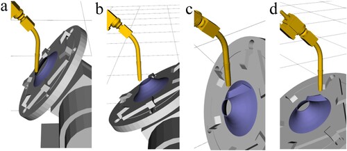
Figure 22. The pose in the real depositing process. (a) Path point 1, (b) path point 2, (c) path point 3 and (d) path point 4.
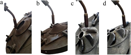
Figure 23. Turbine base planning and depositing process. (a) Path planning result of the first 15 layers, (b) path planning result of the first 30 layers, (c) path planning result of the 54 layers. (d) forming morphology of 15 layers, (e) forming morphology of layer 30 and (f) forming morphology of layer 54.
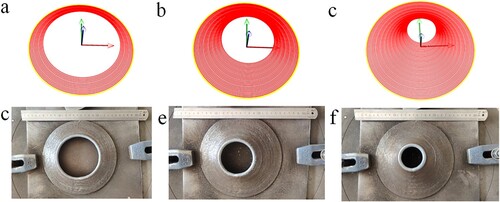
Figure 24. Turbine blade depositing process. (a) Curved layering result of the first layer, (b) curved layering result of the first 10 layers, (c) curved layering result of the 20 layers, (d) Forming morphology of the first layer, (e) forming morphology of the first 10 layers and (f) forming morphology of the 20 layers.
4.3. Forming accuracy analysis
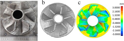
The final forming of the turbine is shown in . In order to verify the forming accuracy, a handheld three-dimensional scanner (ZGScan717) was used to scan the appearance of the turbine. The accuracy of the scanner is 0.02 mm. Compare the scanned model with the standard model in Geomagic software. The error distribution diagram is shown in (d). The standard deviation is 0.95 mm.
Figure 25. Turbine forming appearance and accuracy. (a) Appearance of finished part, (b) scanned model and (c) error distribution.
Sajan Kapil [Citation32] manufactured a impeller by GMA-AM based on planar layering method, and the formed part is shown in . Due to the step effect and molten pool flow, the surface is rough. The results show that the developed curved layering, path planning and joint angle planning of tilting positioner algorithms are effective and powerful. In contrast, the surface forming quality of the turbine processed by the curved surface layering method in this paper is significantly improved. The results show that the developed curved layering, path planning and joint angle planning of tilting positioner algorithms are effective and powerful.
Figure 26. Impeller forming appearance based on planar layering method [Citation32].
![Figure 26. Impeller forming appearance based on planar layering method [Citation32].](/cms/asset/7b391435-ecef-478e-b0c7-a4cc39e24739/nvpp_a_2346289_f0026_oc.jpg)
5. Conclusions
This paper presents a geodesic distance field calculation algorithm based on voxelization and optimized search method, which is developed to realise the curved layering and spatial surface path planning of any STL model. The developed curved layering method is used to carry out GMA additive manufacturing for the turbine with complex surfaces, and the standard deviation of the obtained AM part is 0.95 mm. The verification experiment results show that the surface layering algorithm and spatial equidistant path planning algorithm proposed in this paper can meet the GMA high-precision additive manufacturing of complex parts.
The accuracy of the curved layering algorithm is smaller than the voxel cube edge length L. And the smaller L is chosen, the higher the accuracy of the algorithm, but at the same time the greater the calculation cost. It is recommended that L should be selected from the interval , where l, w, h are the length, width, and height of the printed part model respectively, and e is the forming accuracy of the corresponding process,
is the maximum number of voxel points that can be processed, which depends on the performance of the computer. Future work will consider using tools such as parallel computing and matrix operation libraries to improve the efficiency of the algorithm, and expand the applicable process types and part size range.
Disclosure statement
No potential conflict of interest was reported by the author(s).
Data availability statement
The data presented in this study are available on request from the corresponding author.
Additional information
Funding
References
- Ibhadode O, Zhang Z, Sixt J, et al. Topology optimization for metal additive manufacturing: current trends, challenges, and future outlook. Virtual Phys Prototyp. 2023;18(1):e2181192. doi:10.1080/17452759.2023.2181192
- Alhijaily A, Murat Kilic Z, Paulo Bartolo AN. Teams of robots in additive manufacturing: a review. Virtual Phys Prototyp. 2023; 18(1):e2162929. doi:10.1080/17452759.2022.2162929
- Paolini A, Kollmannsberger S, Rank E. Additive manufacturing in construction: a review on processes, applications, and digital planning methods. Additive Manuf. 2019;30:100894. doi:10.1016/j.addma.2019.100894
- Li Y, Xiong J, Yin Z. Molten pool stability of thin-wall parts in robotic GMA-based additive manufacturing with various position depositions. Robot Comput Integr Manuf. 2019;56:1–11. doi:10.1016/j.rcim.2018.08.002
- Wang C, Wang J, Bento J, et al. A novel cold wire gas metal arc (CW-GMA) process for high productivity additive manufacturing. Additive Manuf. 2023;73:103681. doi:10.1016/j.addma.2023.103681
- Liu D, Lee B, Babkin A, et al. Research progress of arc additive manufacture technology. Materials (Basel). 2021;14(6):1415. doi:10.3390/ma14061415
- Zhao G, Ma G, Feng J, et al. Nonplanar slicing and path generation methods for robotic additive manufacturing. Int J Adv Manuf Technol. 2018;96:3149–3159. doi:10.1007/s00170-018-1772-9
- Huang J, Qin Q, Wen C, et al. A dynamic slicing algorithm for conformal additive manufacturing. Additive Manuf. 2022;51:102622. doi:10.1016/j.addma.2022.102622
- Dolenc A, Mäkelä I. Slicing procedures for layered manufacturing techniques. Computer-Aided Design. 1994;26:119.
- Siraskar N, Paul R, Anand S. Adaptive slicing in additive manufacturing process using a modified boundary octree data structure. J Manuf Sci Eng. 2012;137(01):011007.
- Gokhale NP, Kala P. Development of a deposition framework for implementation of a region-based adaptive slicing strategy in arc-based metal additive manufacturing. Rapid Prototyp J. 2022;28(3):466–478. doi:10.1108/RPJ-10-2020-0246
- Luo N, Wang Q. Fast slicing orientation determining and optimizing algorithm for least volumetric error in rapid prototyping. Int J Adv Manuf Technol. 2016;83(5-8):1297–1313. doi:10.1007/s00170-015-7571-7
- Pérez-Castillo JL, Cuan-Urquizo E, Roman-Flores A, et al. Curved layered fused filament fabrication: an overview. Additive Manuf. 2021;47:102354. doi:10.1016/j.addma.2021.102354
- McCaw JCS, Cuan-Urquizo E. Curved-layered additive manufacturing of non-planar, parametric lattice structures. Mater Des. 2018;160:949–963. doi:10.1016/j.matdes.2018.10.024
- Allen RJA, Trask RS. An experimental demonstration of effective curved layer fused filament fabrication utilising a parallel deposition robot. Additive Manuf. 2015;8:78–87. doi:10.1016/j.addma.2015.09.001
- Shan Y, Shui Y, Hua J, et al. Additive manufacturing of non-planar layers using isothermal surface slicing. J Manuf Process. 2023;86:326–335.
- Chakraborty D, Reddy BA, Choudhury AR. Extruder path generation for curved layer fused deposition modeling. Computer-Aided Design, 2008, 40(2): 235–243.
- Patel Y, Kshattriya A, Singamneni SB, et al. Application of curved layer manufacturing for preservation of randomly located minute critical surface features in rapid prototyping. Rapid Prototyp J. 2015;21(6):725–734. doi:10.1108/RPJ-07-2013-0073
- Hu Z, Hua L, Qin X, et al. Region-based path planning method with all horizontal welding position for robotic curved layer wire and arc additive manufacturing. Robot Comput Integr Manuf. 2022;74:102286. doi:10.1016/j.rcim.2021.102286
- He T, Yu S, Shi Y, et al. High-accuracy and high-performance WAAM propeller manufacture by cylindrical surface slicing method. Int J Adv Manuf Technol. 2019;105(1):4773–4782.
- Dai F, Zhang H, Li R. Process planning based on cylindrical or conical surfaces for five-axis wire and arc additive manufacturing. Rapid Prototyp J. 2020;26(8):1405–1420. doi:10.1108/RPJ-01-2020-0001
- Huang B, Singamneni SB. Curved Layer Adaptive Slicing (CLAS) for fused deposition modelling. Rapid Prototyp J. 2015;21(4):354–367. doi:10.1108/RPJ-06-2013-0059
- Xu K, Li Y, Chen L, et al. Curved layer based process planning for multi-axis volume printing of freeform parts. Computer-Aided Design. 2019;114:51–63. doi:10.1016/j.cad.2019.05.007
- Shan Y, Gan D, Mao H. Curved layer slicing based on isothermal surface - ScienceDirect. Procedia Manufacturing. 2021;53:484–491. doi:10.1016/j.promfg.2021.06.081
- He D, Li Y, Li Z, et al. Geodesic distance field-based process planning for five-axis machining of complicated parts. J Manuf Sci Eng. 2021;143(6):061009. doi:10.1115/1.4048956
- Kraljić D, Kamnik R. Trajectory planning for additive manufacturing with a 6-DOF industrial robot. Proceedings of the 27th international conference on robotics in alpe-adria Danube region (RAAD 2018); 2019.
- Jin Y, Du J, He Y, et al. Modeling and process planning for curved layer fused deposition. Int J Adv Manuf Technol. 2017;91:273–285. doi:10.1007/s00170-016-9743-5
- Lim S, Buswell RA, Valentine PJ, et al. Modelling curved-layered printing paths for fabricating large-scale construction components. Additive Manuf. 2016;12:216–230. doi:10.1016/j.addma.2016.06.004
- Zhao D, Li T, Shen B, et al. A multi-DOF rotary 3D printer: machine design, performance analysis and process planning of curved layer fused deposition modeling (CLFDM). Rapid Prototyp J. 2020;26(6):1079–1093. doi:10.1108/RPJ-06-2019-0160
- Aiyiti W, Zhao W, Lu B, et al. Investigation of the overlapping parameters of MPAW-based rapid prototyping. Rapid Prototyp J. 2006;12(3):165–172. doi:10.1108/13552540610670744
- Ding D, Pan Z, Cuiuri D, et al. A multi-bead overlapping model for robotic wire and Arc additive manufacturing (WAAM). Robot Comput Integr Manuf. 2015;31(1):101–110.
- Kapil S, Joshi P, Kulkarni PM, et al. Elimination of support mechanism in additive manufacturing through substrate tilting. Rapid Prototyp J. 2018;24(7):1155–1165. doi:10.1108/RPJ-07-2017-0139