Qualify-as-you-go: sensor fusion of optical and acoustic signatures with contrastive deep learning for multi-material composition monitoring in laser powder bed fusion process

ABSTRACT

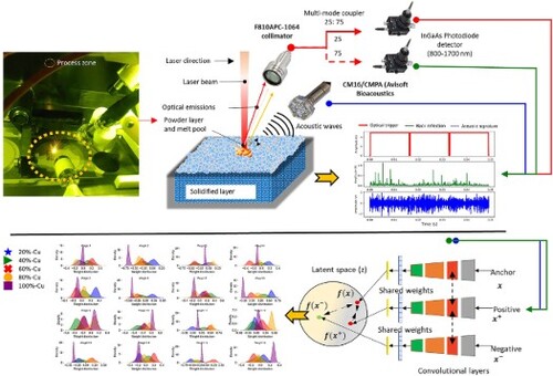
Growing demand for multi-material Laser Powder Bed Fusion (LPBF) faces process control and quality monitoring challenges, particularly in ensuring precise material composition. This study explores optical and acoustic emission signals during LPBF processes with multiple materials, addressing challenges in process control and ensuring accurate material composition. Experimental data from processing five powder compositions were collected using a custom-built monitoring system in a commercial LPBF machine. The research categorised signals from LPBF processing various compositions, enhancing prediction accuracy by combining optical with acoustic data and training convolutional neural networks using contrastive learning. Latent spaces of trained models using two contrastive loss functions, clustered acoustic and optical emissions based on similarities, aligning with five compositions. Contrastive learning and sensor fusion were found to be essential for monitoring LPBF processes involving multiple materials. This research advances the understanding of multi-material LPBF, highlighting sensor fusion strategies’ potential for improving quality control in additive manufacturing.

GRAPHICAL ABSTRACT

KEYWORDS:

• Laser powder bed fusion
• multi-material process monitoring
• acoustic emission
• optical emission
• contrastive learning

1. Introduction

During the last few years, there has been an increased interest in the Laser Powder Bed Fusion (LPBF) process for a series of engineering alloys, including stainless steel, nickel-based superalloys, Ti6Al4 V, aluminium and copper alloys[1–5]. One of the current trends is the fabrication of multi-material structures, consisting of at least two different alloys, by depositing one alloy over the other. One particular case of multi-material structures is the printing of compositionally functionally graded alloys (FGAs), where the transition from one alloy to the other is done by depositing layers, consisting of intermediate compositions, between the layers of the individual alloys. This approach provides the advantage of constructing structures with gradient thermophysical properties in one or even two directions, depending on the powder feeding capacities of each LPBF machine, with the transition taking place on the micrometer scale (same scale as the powder layer thickness). Among the different combinations of material to be fabricated as bimetal or multi-material structures, the key role has the combination of (stainless) steel with pure copper and its alloys, as the combination of high strength and corrosion resistance of the former, together with the high thermal and electrical conductivity of the latter, constitute their multi-material structures as possible candidates for fusion reactors, heat exchangers and casting moulds [6–9]. However, there are still critical challenges regarding the fabrication of steel-copper multi-material structures, including crack formation, due to the penetration of copper on the austenite grain boundaries and the formation of lack of fusion defects on copper-containing parts due to its high thermal conductivity and its high laser reflectivity. In that regard, monitoring compositionally functionally graded structures made of steel and copper is vital for tracking the phenomena mentioned above as a function of the compositional step.

Evaluating the quality of components produced using Additive Manufacturing (AM) ensures its dependability and performance. Defects such as porosity resulting from the LPBF printing process can significantly impede the mechanical properties and weaken the performance of as-printed components, potentially challenging the reliability and reproducibility of the printed parts[10]. Traditional methods such as CT (Computed Tomography), ultrasonic inspection and labour-intensive cross-sectional analysis continue to be widely utilised for comprehensive assessments [11–15]. These post-mortem techniques are indispensable for guaranteeing the excellence and reliability of AM processes. However, they do come with certain limitations. Post-mortem techniques cannot detect defects in real time, potentially resulting in material wastage if issues are only discovered after the printing process has concluded [16]. Furthermore, they cannot make immediate adjustments during the printing process itself. Post-mortem analysis can be time-consuming, often requiring the disassembly of printed components for thorough inspection. In contrast, real-time monitoring offers instantaneous feedback, enabling more efficient resource utilisation and faster decision-making. Real-time monitoring takes a proactive stance by addressing issues as they occur, thereby reducing material waste and minimising the necessity for post-processing. Analysing temperature signals, image signals, and spectral signals from the process zone facilitates a better understanding and tracking of complex thermal-physical-chemical-metallurgical processes [17]. Achieving real-time monitoring in LPBF requires a well-coordinated system of sensors, data acquisition and control Machine Learning (ML). Machine learning and statistical analysis can identify patterns, connections, and optimal printing settings, resulting in improved and more cost-effective part production [18]. Moreover, the data collected from monitoring can be leveraged to continuously enhance the printing process. Additionally, process monitoring maintains a detailed digital record of each printed part, including its specifications and quality assessments, which is a valuable asset in critical industries such as aerospace and medical applications [19]. Incorporating cutting-edge sensors overlooking the LPBF process zone marks a significant step toward realising real-time monitoring capabilities [20,21]. This allows us to observe the perturbations of the emissions originating from the process zone as the laser interacts intricately with the powder bed. These emissions can be systematically categorised into two primary types: optical emissions and acoustic emissions [22]. Examining optical emissions closely provides abundant insights into the process zone's temporal and spatial aspects [23]. Temporally, they enable us to detect subtle intensity fluctuations during the process [24]. From a spatial standpoint, they offer a unique perspective on the changing shape of the process zone [25]. Furthermore, it is essential to acknowledge that the dynamic behaviour of the melt pool itself induces reverberations within the surrounding atmospheric medium as acoustic pressure waves [26]. These reverberations carry with them intricate temporal patterns that encapsulate vital information concerning the intricate dynamics of the process [27]. In essence, these sensors serve as the keen eyes and sensitive ears of the LPBF process, furnishing us with a continuous stream of real-time data pertaining to pivotal aspects such as temperature variations, the fluid dynamics of the melt pool, and the overall condition of the process zone [28–31].

The analysis of secondary electromagnetic emissions from the melt pool presents a valuable avenue for gaining insights into its condition [32]. By observing the size and shape of the melt pool, one can extract valuable information regarding energy input and laser scanning strategies. Any deviations from the expected melt pool shape can signal potential process instability [33]. Furthermore, maintaining a vigilant eye on temperature distribution within the melt pool is imperative, as temperature variations can indicate incomplete melting, overheating, or irregular cooling. Optical detectors sensitive to the infrared (IR) wavelength are the preferred choice for monitoring temperature, capturing thermal radiation emitted by the melt pool throughout the LPBF process [34]. Bertoli et al. showed how high-speed imaging of LPBF could be used to study laser-powder interaction, melt pool evolution, and cooling rates in 316 L powder layers, comparing gas and water-atomised feedstock materials [35]. Zhichao Yang et al. explored changes in the molten pool, spatter formation mechanisms, and powder flow in additive manufacturing processes, utilising a high-speed camera and grounded in the analysis of gas-solid mixed flow characteristics [36].

Infrared imaging offers real-time temperature data for simulating temperature distribution within the melt pool, identifying trends in column and overhang regions, and reducing layer-to-layer temperature variations in LPBF compared to experimental data [37]. It’s crucial to recognise that imaging datastreams have drawbacks, including lower temporal resolution and higher computational demands. As an alternative in optical detection-based sensing, detectors such as photodiodes and pyrometers are worth considering [24,38–41]. LPBF melt pools were monitored using in situ high-speed pyrometry, facilitating probabilistic pore formation predictions and the detection of conduction-keyhole mode transition, validated by metallography [38]. While pyrometry offers a detailed perspective of the process zone with high temporal resolution, its spatial resolution is limited. [42]. Moreover, these detectors require fewer computational resources for processing, and their integration with ML techniques has further improved the reliability of process monitoring solutions [41,43]. Melt pool perturbations occurring within the 10–100 μs time frame [32–34] present a distinctive challenge in the context of effective monitoring [44–46]. Ensuring that sensors possess the necessary attributes of swift responsiveness and robustness against dynamic fluctuations is crucial [47]. Air-borne Acoustic Emission (AE) sensors prove to be well-suited for meeting this essential requirement. These sensors offer a dependable and cost-effective solution because they can detect and capture the rapid reverberations from the melt pool transmitted to the surrounding atmosphere with high temporal precision, as corroborated by previous studies [48]. Across LPBF regimes, it has been proven that the temporal characteristics of air-borne AE waveforms exhibit variability [27]. Utilising acoustic sensors offers a swift and efficient avenue for extracting valuable insights from the LPBF process zone by scrutinising waveform data, facilitating the characterisation of the fundamental physical mechanisms at play. Notably, this approach places lower demands on computational resources and is a more cost-effective option against alternative sensor technologies. In the realm of sensing, there is an emerging trend involving the fusion of information derived from two or more distinct sensing technologies aimed at achieving a more comprehensive understanding. The authors’ prior research has demonstrated that a custom-built optical spectral detector, designed to be sensitive across three distinct wavelength regions encompassing visible, infrared, and laser wavelengths, has successfully enabled the monitoring of LPBF processes [24]. Furthermore, it was observed that optical detectors linked to the laser wavelength yielded more information richness. Gaikwad et al. [49] employed a data fusion approach to enhance flaw detection by capturing melt pool information through two high-speed video cameras and a temperature field imaging system. These data sources were utilised to extract low-level melt pool characteristics, which were then employed for predicting porosity type and severity. Sharing complementary information among these sensors ultimately enhances their correlation with anomalies. This development paves the way for achieving high confidence in the industrialisation of real-time monitoring systems.

The intricate and nonlinear nature of data obtained from sensors within the process zone poses a significant challenge, making real-time decision-making by human operators difficult. The need for continuous decision-making in an automated system is crucial. Integrating signal preprocessing and ML analysis pipelines is a powerful solution to address this challenge. Statistical features from optical and thermal sensors, obtained through signal processing, can be used with ML algorithms such as Decision Trees (DT) and K-nearest neighbours (KNN) for part quality assessment [50]. Statistical data derived from acoustic signals has enabled classifiers like linear Support Vector Machine (SVM), Random Forest (RF), and logistic regression to effectively distinguish different processing regimes in LPBF [48,51]. Nevertheless, the reliability of the ML model, trained on manually extracted features, is contingent on human-selected features, which can be a limitation in such approaches. Recent research has shown a growing interest in using deep learning, particularly Convolutional Neural Networks (CNNs), to monitor the LPBF process. Unlike traditional ML methods, DL can work with minimal data preprocessing. Neural network architectures such as deep belief networks, spectral convolutional networks, and training strategies like transfer learning were utilised. Under specific parameters, they were trained on air-borne acoustic emissions originating from the process zone during laser processing. This training led to identifying defective regimes, allowing for the distinction between anomalies and correct conduction regimes [52–54]. CNNs excel in identifying LPBF anomalies (porosity, density variations, delamination) using various sensor data [52,54–59]. Furthermore, the continuous learning capacity of these models ensures adaptability to changing conditions, holding the promise of a transformative impact on the AM industry by ushering in intelligent and data-driven 3D printing processes [60,61].

As the monitoring process for LPBF in real-time continues to advance, research into monitoring the LPBF process involving multiple materials is still in its early stages. While the authors’ prior research has demonstrated the effectiveness of CNN-based transfer learning in learning transferable features from one material to another with minimal network training time [56], the simultaneous exploration of compositions involving two different materials remains relatively unexplored, particularly in terms of monitoring. This study aims to address this research gap by introducing a novel temporal sensor fusion method. This method is designed to synchronise and align data from multiple sensors across the entire build volume, utilising optical emissions within the laser spectral range and acoustic data from the process zone. Furthermore, it's worth noting that despite the availability of various ML approaches, only a limited number of studies have explored contrastive learning architectures, which are known for their efficiency in handling complex tasks. This efficiency is particularly relevant to monitoring multi-materials, where the process emissions are intricate. The primary strength of contrastive learning lies in its ability to detect differences in process zone information, thereby capturing variations in compositional quality. This robust methodology can then be applied to predict precise compositional control at specific locations.

This paper is divided into five sections. Section 1 presents a concise overview of the multi-material LPBF process and emphasizes the importance of process monitoring. Section 2 offers a brief theoretical explanation of CNN-based contrastive learning techniques, specifically focusing on circle loss and triplet loss. Section 3 introduces the experimental setup, sensor configuration, data collection pipeline, and initial statistical analysis of the two data streams utilised in this study. Section 4 delves into the significance of employing sensor fusion strategies when dealing with multiple materials and discusses the challenges associated with training them within conventional CNN frameworks. Section 5 explores an alternative approach that combines contrastive learners with sensor fusion strategies and evaluates the feasibility of the proposed methodologies. Finally, Section 6 provides a comprehensive review of the paper's findings.

2. Theoretical basis

In contrastive learning, the goal is to bring similar data samples closer together within a lower-dimensional embedding space while maximising the separation between dissimilar data points [62]. This embedding space represents a lower-dimensional representation computed using a CNN. The core methodology of contrastive learning marks a significant departure from conventional approaches. Unlike conventional methods of training a network on a data stream and its corresponding ground truth labels, this innovative technique operates with pairs of data streams, which can be similar or dissimilar. These pairs are fed into the network using a specific training procedure tailored for contrastive learning [63]. This approach proves particularly valuable in training deep neural networks for representation learning tasks, where the network's weights are dynamically updated during training. The trained contrastive model produces a refined lower-dimensional representation of the input data, which can be employed for diverse applications such as classification, segmentation, and verification. It is important to note that the choice of the loss function used in contrastive learning and the associated training strategy plays a pivotal role in determining the technique's effectiveness [64]. In this work, we explore the use of loss functions such as triplet and circle loss to further enhance the performance and capabilities of contrastive learning in various applications.

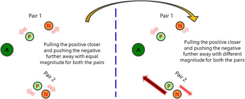
In the context of triplet loss, a set of data triplets is fed into a network model consisting of an anchor $\left(a\right)$, a positive $\left(p\right)$, and a negative $\left(n\right)$data sample. The anchor data sample acts as a reference point, while the positive and negative data samples are drawn from the same and different categories. The purpose of triplet loss is to minimise the distance between the low-dimensional representations of the anchor and the positive $\left(p\right)$ while simultaneously maximising the distance between the anchor and the negative $\left(n\right)$ [65]. To make accurate predictions, it is essential for the distances between the anchor and the positive data sample (d+) and between the anchor and the negative data sample (d-) to be smaller and larger, respectively, as shown in Figure 1. The network model is employed in the training process with triplet loss, and three instances of this model share the same architecture and weights [66].

Figure 1. Contrastive learning using Triplet loss.

The triplet loss is computed at each training iteration by comparing the lower-dimensional representations obtained from the output layers of the network. Subsequently, the network’s weights are adjusted to minimise this loss. Mathematically, the loss value can be calculated as shown in Equation (1), (1) $\mathcal{L}=max\left(d\left(a,p\right)-d\left(a,n\right)+m,0\right),$(1) where d is a function to measure the distance between these three instances of the model and m is margin.

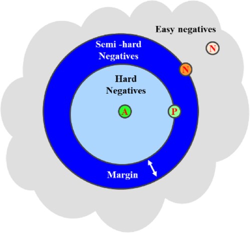
Without interference from negative examples, triplet loss does not alter the distances within a positive cluster. This is because triplet loss aims to establish a margin between the distances of negative and positive pairs, ensuring a clear delineation between similar and dissimilar data points [67]. In the context of Circle Loss, it is a crucial contrastive learning loss function aimed at enhancing the embedding space by emphasizing both intra-class similarity and inter-class discrimination. Circle Loss introduces circular boundaries around data points in the embedding space, with trainable radii for each circle. Despite its name, ‘Circle Loss’ represents the concept of defining margins within the embedding space rather than geometric circles. Each data point is associated with a circle (or hypersphere in higher dimensions) with an adjustable radius. During training, Circle loss encourages similar data points to cluster within their designated circles and pushes dissimilar points to expand beyond these boundaries. [68].

Circle Loss is a mathematical method that penalises instances outside their correct circles. Its aim is to minimise the distances between similar data points and the centres of their respective circles while maximising the distances between dissimilar points and the boundaries of those circles. This approach encourages the formation of distinct clusters for different classes, promoting the closeness of embeddings within their respective circles. To illustrate the effectiveness of Circle Loss, consider a scenario where two pairs have an equal margin between positive and negative elements, but one pair is positioned close to the anchor while the other is considerably distant. Traditional Triplet Loss treats both pairs equally, adjusting the positive and negative elements similarly. However, Circle Loss introduces a flexible optimisation strategy by assigning unique penalty strengths to each similarity score, introducing independent weighting factors. This preference for equilibrium avoids extreme cases where the negative element is very close or the positive element is excessively distant [69]. A compelling illustration as shown in Figure 2, further elucidates the efficacy of circle loss. Beyond its flexibility and improved convergence characteristics, circle loss demonstrates adaptability by using different penalty strengths for each similarity score. Circle loss emerges as a powerful tool in contrastive learning, enhancing discriminative capacity and improving the quality of learned representations across various computer vision applications.

Figure 2. Contrastive learning using circle loss.

In essence, this study aims to showcase how contrastive learners, employed for feature extraction in monitoring laser powder bed fusion (LPBF) processes, particularly in scenarios involving multiple materials, effectively manage the complexities within sensor data. The presence of multiple materials makes traditional classification tasks challenging, highlighting the importance of contrastive learning in this area. Previous literature has not addressed these challenges encountered by conventional classifiers because they didn't focus on handling intricate data from multimaterials. Our main goal is to bridge the gap between conventional classifiers and the specific requirements of complex, multi-material LPBF processes, ultimately improving the efficiency of process monitoring and control in multi-material LPBF setups.

3. Experimental setup, materials, data acquisition and methodology

3.1. Experimental setup

The experimental setup involved the utilisation of a SiSMA MySINT 100 LPBF machine with specific parameters (wavelength λ = 1070 nm, spot size diameter = 55 μm, maximum power P_max = 200 W). Argon gas was introduced into the build chamber at atmospheric pressure to establish an inert environment. Additionally, we incorporated a custom in-situ AE and optical sensing system inside the processing chamber, illustrated in Figure 3. This schematic representation visually illustrates the process of collecting AE data and optical emissions as employed in our study. We employed a fixed-focus collimator of the F810APC-1064 type from Thorlabs to capture optical emissions originating from the laser irradiation zone, which had high transmission only to wavelengths between 1050 and 1074 nm. This collimator was deliberately positioned off-centre and oriented at a 75° angle, 12 cm away from the top surface of the build plate. The collimator is strategically positioned with a shorter working distance, offering a nearly direct view of the process zone. It has a field of view of 24 mm tailored to capture emissions from this area. Additionally, the field of view collimator on the baseplate is larger than the actual printing area of the cube (10 mm). This configuration is meticulously designed to optimise the collection of relevant signals, compensating for the off-axis positioning of the photodiode. The optical signals collected were then split into two parts using a 25:75 multi-mode fibre splitter. One-quarter (25%) of the signal was directed to a photodiode (PDA20CS2, 800–1700 nm; Thorlabs) and routed to the first channel of the Data Acquisition (DAQ) system, dedicated to capturing optical emissions resulting from the laser-powder bed interactions. The remaining three-quarters (75%) of the signal was directed to another photodiode (PDA20CS2, 800–1700 nm; Thorlabs) and subsequently routed to the second channel. The third channel was exclusively reserved for acquiring acoustic data. Although the two photodetectors are sensitive to a broad range (800–1700 nm), the nature of the coating used in the collimator restricts the photodiode detector readings to intensity variations between 1050 and 1074 nm. The study utilised an air-borne AE sensor, specifically the CM16/CMPA model from Avisoft Bioacoustics, as depicted in Figure 3. This sensor had a frequency response range of 0–150 kHz. Notably, while the AE detector maintains uniform sensitivity across this frequency range, it exhibits directionality. Consequently, the microphone was mounted at an angle of 60° degrees to optimise its performance.

Figure 3. Schematics of the proposed sensing system comprising photodiode and AE sensors.

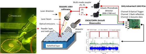
The data acquisition process was triggered based on the output of the optical channel when the laser interacted with the powder bed, as detected by the photodiode in the first channel. This photodiode converted optical signals into an analogue voltage signal, directly proportional to the intensity detected. When this voltage signal exceeded a predefined threshold (set at 0.5 V in our case), it triggered the DAQ card to capture data from both channels. All three channel signals were concurrently captured using an Advantech 1840 PCIe data acquisition card (Advantech, USA), which had a dynamic range of ±5 V and a sampling rate of 400 kHz. This sampling rate was chosen to adhere to the Nyquist-Shannon theorem and match the frequency response of the AE sensor. The synchronisation of the optical and AE channels ensured precise coordination, where the photodiode linked to the first channel consistently generated an intensity exceeding the upper saturation limit of 5 V during each laser exposure to the powder bed, resulting from its optimised gain settings. This consistent intensity pattern led to the formation of a square wave pattern, delineating distinct phases of the laser exposure. Within this structured waveform, the AE signatures and photodiode signals captured during each phase correspond to individual scan tracks, providing a detailed representation of the process dynamics. These signals were meticulously processed to extract valuable insights. Moreover, the collected AE and photodiode signals from the second and third channels underwent specific windowing procedures, precisely aligned with the active or high phase of the laser channel, i.e. the square wave pattern. This strategic windowing ensured that the relevant data pertaining to each laser exposure phase were isolated, enhancing the accuracy and relevance of subsequent analyses. As a result of this synchronised and structured data acquisition approach, a comprehensive dataset was compiled, covering AE windows and optical intensity data meticulously correlated with the laser wavelength. This rich dataset served as a valuable resource for in-depth analysis and interpretation of the underlying processes occurring within the laser-powder interaction zone.

3.2. Materials

Two different powders have been used to fabricate steel-copper multi-material structures: 316L stainless steel provided by Oerlikon and CuCrZr powder provided by Eckart. The chemical compositions of the two powders are given in Tables 1 and 2, respectively.

Table 1. Chemical composition of the 316L powder feedstock provided by Oerlikon.

Weight percent (nominal)
Fe	Cr	Ni	Mo	C	Other
Balance	18	12	3	<0.03	<1.0

Table 2. Chemical composition of the CuCrZr powder feedstock provided by Eckart.

Weight percent (nominal)
Cu	Cr	Zr	Fe	Si
Balance	0.96	0.12	0.021	<0.004

The powders were initially blended using a powder mixing device (Turbula, WAB AG Maschinenfabrik), where 100 g of each powder premixture underwent individual mixing for one hour. Six distinct compositions were prepared, and for each composition, 20 wt. % CuCrZr powder was consistently added, as outlined in Table 3. A cubic structure with dimensions of (1 × 1 × 1.7 cm³) was constructed using 316L powder, and 100 layers were printed for each of these compositions. The multi-material cube structure was manufactured using two different parameter sets. The cubes were printed using a bidirectional scanning strategy with a 90-degree rotation, and no contour scanning was employed.

Table 3. LPBF process parameters on building the cubic structure.

	Laser Power (W)	Scan speed (mm/s)	Hatch distance (μm)	Layer thickness (μm)	Label
316L wt.%	125	750	80	30	100%-316L
80-20 316L-CuCrZr wt.%	200	600	90	30	20%-Cu
60-40 316L-CuCrZr wt.%	200	600	90	30	40%-Cu
40-60 316L-CuCrZr wt.%	200	600	90	30	60%-Cu
20-80 316L-CuCrZr wt.%	200	600	90	30	80%-Cu
CuCrZr wt.%	200	600	90	30	100%-Cu

A single set of parameters was applied for 316L stainless steel, whereas a different set was utilised for printing all steel-copper premixtures. It is crucial to emphasize that consistent parameters were employed for printing the copper-containing powders. This methodology was chosen to prioritise the evaluation of compositional effects and to ensure that any variations in printing parameters between different premixtures would not influence the research results. Due to the distinct characteristics of the process space for 100% 316L stainless steel in comparison to the copper-containing alloys, it was chosen not to include the former in our data analysis. This decision was guided by the author's prior research indicating that acoustic emissions from 316L stainless steel are likely to differ significantly from those of the alloy combinations containing copper [48]. Subsequent to printing each composition, the LPBF machine was meticulously cleaned, and a fresh powder premixture was loaded into the supply cylinder. After printing, the sample was separated from the build plate using Electrical Discharge Machining. Cross-sectional analyses were conducted using optical microscopy to verify the presence of the five distinct compositional powders within the constructed cuboid. These sections were cut perpendicular to the scan tracks and then prepared through grinding and polishing procedures in accordance with established metallographic preparation standards. As shown in Figure 4, the differing levels of build density, porosity, and voids observed in each region confirmed that the selected laser powers and scanning speeds successfully produced the intended results.

Figure 4. Cross section of the gradiently printed cube.

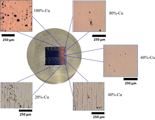
However, it is essential to recognise the occurrence of cracking in two specific compositional combinations, particularly those containing 20 wt. % Cu and 40 wt. % Cu. These instances of cracking are a common observation in 316L-Cu bimetal structures [70–72] and are typically attributed to the infiltration of liquid copper into the grain boundaries of the austenite phase. Interestingly, these cracks do not manifest in premixtures with higher Cu content (60 wt. % Cu and 80 wt. % Cu). This variation can be ascribed to two factors: first, the consistent application of the same printing parameters for all premixtures (potentially resulting in lower Volumetric Energy Density Values for 20 wt. % Cu and 40 wt. % Cu, thereby reducing the likelihood of crack formation); and second, the formation of Body-Centered Cubic (BCC) ferrite in the 60 wt. % Cu and 80 wt. % Cu gradient compositions. As demonstrated in prior research by Chen et al. [73], this ferrite formation enhances the resistance of the steel to intergranular penetration by liquid copper.

A comprehensive investigation of these cracking phenomena falls beyond the scope of this current paper and will be addressed in future research publications. Furthermore, as the authors have already demonstrated the ability of acoustic emission (AE) signals to distinguish between the two alloys [48], our primary focus in this study was on exploring different compositions rather than different alloys. This study primarily focuses on compositional monitoring rather than defect identification. The objective is to analyse and monitor five different material compositions within the same process parameter space to understand and optimise the additive manufacturing process. It's important to note that this study does not aim to detect anomalies or defects within the material compositions. Instead, the emphasis is on monitoring and analysing the compositional variations throughout the additive manufacturing process. Additionally, the nature of this study precludes the possibility of anomaly detection, as all considered compositions are relevant within the scope of this investigation. This study centres on compositional monitoring, aligning with the core research objectives. Therefore, the analysis in this work centres on five distinct compositions, considering the blended version of CuCrZr with 316L and only CuCrZr.

3.3. Data acquisition pipeline and dataset

During the fabrication of the cube, incorporating five distinct powder compositions in a continuous sequence, the optical signal, as detected by the photodiode in the first channel, consistently exceeds the 0.5 V threshold at the onset of each layer. This threshold crossing serves as the triggering event for the commencement of signal acquisition from the AE sensor, which is dedicated to the specific layer under consideration. Throughout the scanning process of each layer, meticulous control is exercised over the photodiode sensor's gain, interconnected with channel 1, to sustain saturation at the precise threshold of 5 V. The harmonisation of the remaining optical and AE channels, specifically the second and third channels, allows for compiling a comprehensive dataset encompassing AE windows and optical intensity data correlated with the laser wavelength. Notably, each of these windows adheres to a synchronised temporal scale, thus corresponding precisely to individual scan tracks. Subsequently, these complex signals undergo a meticulous segmentation process into discrete 12.5 ms windows, each containing 5000 data points. Following this segmentation procedure, the AE signals are subjected to offline low-pass Butterworth filtering, adopting a predetermined cut-off frequency of 150 kHz. Notably, the selection of this particular cut-off frequency aligns judiciously with the documented frequency response specification of the AE sensor, and this criterion is consistently upheld across all experimental scenarios and cube variations. For a more comprehensive insight into the dataset underpinning this study, we encourage referring to Table 4.

Table 4. The total number of 12.5 ms (5000 data points) AE and optical windows that were extracted during the fabrication of the cube.

Category	Windows per Acoustic and Optical Channel
20%-Cu	5448
40%-Cu	6205
60%-Cu	5457
80%-Cu	5457
100%-Cu	5457

3.4. AE signal processing

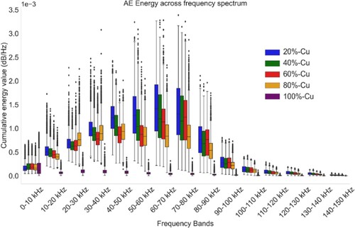
The energies corresponding to fifteen distinct frequency bands (ranging from 0–10 kHz, 10–20 kHz, 20–30 kHz, 30–40 kHz, 40–50 kHz, 50–60 kHz, 60–70 kHz, 70–80 kHz, 80–90 kHz, 90–100 kHz, 100–110 kHz, 110–120 kHz, 120–130 kHz, 130–140 kHz, and 140–150 kHz) were computed using the periodogram method for all the windows in the dataset. This analysis investigated the characteristics of the AE waveform signals associated with five distinct powder compositions in the frequency domain. As illustrated in the accompanying figure, the cumulative energy values for the various regimes are clearly depicted across these fifteen frequency bands. The figure reveals that the majority of energy components in all regimes are primarily clustered within the frequency range below 100 kHz, regardless of the powder distribution used. Notably, when processing copper, there is a distinct reduction in the peak energy of AE waves compared to other compositions. This occurrence can be linked to the distinctive optical properties intrinsic to copper. Additionally, as we analyse compositions with varying copper percentages, noticeable patterns emerge within each specific frequency range. The comparative analysis of cumulative energy distribution across these fifteen distinct frequency bands substantiates the existence of pronounced deviations in the energy content of AE waves. These deviations are attributed to the intricate dynamics of the melt pool, intricately linked to the specific powder composition in use. Additionally, the significant standard deviation underscores the stochastic behaviour of air-borne acoustic emissions owing to the process dynamics in multi-material laser interaction, emphasizing the necessity of employing complementary sensing modalities for comprehensive process monitoring (Figure 5).

Figure 5. Comparison of cumulative energy content between fifteen frequency bands for five compositions used in this study.

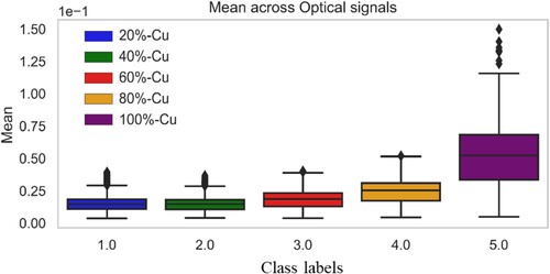
To establish an initial confirmation of how changes in powder composition have influenced the optical intensity corresponding to the laser wavelength within the process zone, the time-domain analysis involved resolving the windows associated with each regime. The Root Mean Square (RMS) was initially computed from the optical channel corresponding to the laser wavelength for each powder composition. The comparison of RMS distribution within these powder compositions, as depicted in Figure 6, reveals areas of substantial overlap and an observable increasing trend about the mean value as the concentration of copper in the composition increases. This trend aligns intuitively with the optical properties inherent to copper. However, it's crucial to recognise that Category 5 represents pure copper, which inherently possesses distinct optical properties on the laser wavelength and high reflectivity compared to compositions with gradients of 316L and copper. Consequently, the data spread in Category 5 exhibits more pronounced variability, leading to higher upper and lower standard deviations.

Figure 6. Distribution of RMS features for five compositions used in this study.

The presence of statistically significant differences in both the optical and acoustic data is a compelling rationale to leverage these signatures for real-time monitoring of powder composition when combined with ML techniques.

4. Deep-net architecture

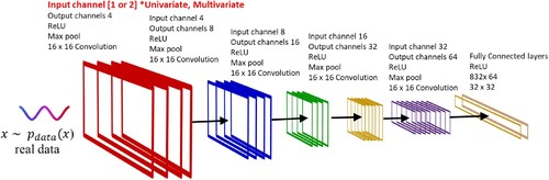
In this section, we delve into designing and training three CNN models using the sensor signals discussed in the previous section in conjunction with the ground truth labels. Our primary objective here is to achieve precise classification across five different compositions. These models are identified as CNN-1(a), CNN-1(b), and CNN-2, each with unique specialisations and architectural considerations. CNN-1(a) was exclusively trained on acoustic data, while CNN-1(b) focused on processing the photodiode signal. The CNN architectures were implemented using the PyTorch package from Meta (USA) [74]. CNN-1(a) and CNN-1(b) possess an identical architecture designed to handle univariate data streams. This decision was reached through a comprehensive search process and was guided by previous research findings [24]. Our goal was to uphold consistency with the architecture design established in our prior works, which have proven effective in analogous applications. This strategy ensures continuity and simplifies the comparison and validation of results across various studies. As a result, this architecture consists of five convolutional layers and three fully connected layers, as illustrated in Figure 7. In the CNN implementation of the presented work, the direct utilisation of the 1-D signal without conversion into a 2-D spatial form reduces parameters, enables real-time processing, and lowers computation costs, optimising efficiency for signal analysis tasks.

Figure 7. Overview of the proposed CNN architecture for the supervised classification of five different compositions.

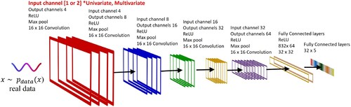
The architectural composition of CNN-1(a) and CNN-1(b) is characterised by five 1D convolutional layers, each employing a kernel size of 16. The number of kernels gradually increases, starting with four in the initial layer and reaching 64 in the fifth layer. Following each convolutional layer, a max-pooling operation with a kernel size of two is systematically applied to down-sample the feature map. For the final classification, we purposefully employ a set of three fully connected layers, all utilising the Rectified Linear Unit (ReLU) activation function. In this study, we thoughtfully partition the dataset into training (60%), validation (10%), and testing (30%) subsets. This division serves the dual purpose of training the model and subsequently evaluating its performance. The input dimensions of the initial CNN layer are precisely defined as a tensor of size N × 5000 × 1, with N explicitly set to 256 as the batch size. During training, the model's output generated by both CNN-1(a) and CNN-1(b) is compared to the ground truth labels using the cross-entropy loss function. The training process spans 300 epochs, with all 300 epochs taking 1.5 h during training. The learning rate undergoes periodic adjustments every 50 epochs to facilitate optimal convergence. It begins at 0.001 and is then multiplied by a gamma value of 0.5. To prevent overfitting, batch normalisation is consistently applied across all layers of the CNN architecture. The datasets are carefully randomised between epochs, and the chosen training optimiser is AdamW. A 5% dropout is incorporated during the training process between each cycle to enhance model generalisation. It is worth noting that CNN-1(a&b) is trained on a high-performance Graphics Processing Unit (GPU), specifically the Nvidia RTX Titan. The total number of tuned parameters for CNN-1(a&b) is calculated to be 0.1 million. For a detailed summary of the training parameters, please refer to Table 5. The total number of tuned parameters for CNN-1(a&b) is calculated to be 0.1 million. It is important to note that while our selection of architecture and hyperparameters is informed by prior knowledge and empirical experimentation, there remains room for further optimisation.

Table 5. Training parameters of the three CNN models trained supervisedly with cross-entropy loss.

Training parameters	CNN-1
Analysis type	Classification
Solver used	‘AdamW’
Learning rate used	0.01
Training epochs	300
Batch size	256
Dropout	5%
Loss function	Cross entropy
Shuffle	Every-epoch
Labelled dataset	60% Training, 30% testing, 10% Validation
Trainable weights	0.60 million

The training progress of CNN-1(a), as displayed in Figure 8(a), provides a comprehensive visualisation of the model's training loss values throughout 300 closely monitored training epochs. This visualisation emphasizes the model's ability to understand the underlying data distributions. Additionally, the gradual improvement in training accuracy, depicted in Figure 8(b), underscores the model’s consistent and effective generalisation for classification on the AE signal test data subset.

Figure 8. Inference plots after model training (a) Learning curves illustrating model training progress: evaluating performance and convergence of the three models (CNN-1(a), CNN-1(b) and CNN-2) (b) Visualisation of performance prediction the three trained models (CNN-1(a), CNN-1(b) and CNN-2) on the test dataset.

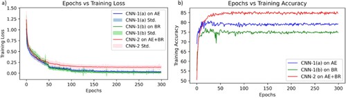
The classification results on the test data of CNN-1(a), precisely tabulated as a confusion matrix in Table 6, offer a comprehensive overview of the model's classification performance. CNN-1 demonstrated an average classification accuracy of 79.4% on the test set. At the same time, a CNN-1(b) model was trained under supervised conditions and designed to follow the exact architectural blueprint of CNN-1(a). However, CNN-1(b) was configured to process the photodiode signal as input data. To ensure consistency and fairness in the comparison, we initially employed the same training parameters and methodology used for training CNN-1(a). The training progress of CNN-1(b), as illustrated in Figure 8(a), closely mirrored the training progress observed in CNN-1(a). This similarity in training loss values suggests that both models underwent a comparable learning process. However, when it came to the real test – evaluating their performance on the test dataset – it became evident that CNN-1(b)'s classification accuracy was markedly lower, as tabulated in Table 6. In fact, it was approximately 74.7%, which is lower than what CNN-1(a) achieved when predicting using AE signals.

Table 6. Table shows accuracies for predicted label (wear classes) vs true label (ground truth) on five classes.

	Ground truth
Classification (accuracy [%])	20%-Cu	40%-Cu	60%-Cu	80%-Cu	100%-Cu
20%-Cu	72.9	22	2.2	2.9	0
	69.9	25.1	3.3	1.7	0
	79.8	18.2	0.9	1.1	0
40%-Cu	23.2	62.5	11.2	3.1	0
	21.6	56.4	18.4	3.6	0
	17.6	73	7.4	2	0
60%-Cu	2.5	12	76.2	9.1	0.2
	2.5	16.8	67.2	13.5	0
	0.7	7.8	81.8	9.7	0
80%-Cu	2.3	2.8	8.8	85.7	0.4
	3.2	2.9	13.6	80	0.3
	0.8	1.7	9.1	88.4	0
100%-Cu	0	0	0.3	0	99.7
	0	0	0	0.3	99.7
	0	0	0	0.3	99.7

Tables for the classification accuracy results using the three CNN classifier models (CNN-1(a), CNN-1(b) and CNN-2). The classification results in each cell from top to bottom are for: CNN-1(a), CNN-1(b) and CNN-2. All values are in %.

While both CNN-1(a) and CNN-1(b) exhibited limited proficiency in their respective univariate data domains, the potential for enhanced classification performance was explored through sensor fusion. A multivariate model, CNN-2, was meticulously trained to pursue this objective. CNN-2 incorporated both acoustic emission and photodiode signal data streams by introducing two channels in its first layer therefore the input dimensions of the initial first layer is defined as a tensor of size N × 5000 × 2. The training parameters and protocols, mirroring those used for CNN-1(a) and CNN-1(b), were similarly applied to CNN-2. The training loss values of CNN-2, as depicted in Figure 8(a), showcase its impressive ability to decode complex data distributions. Notably, CNN-2 achieved a higher classification accuracy of 84.5% on the test set, as depicted in Figure 8(b) and Table 6, surpassing the performance observed in CNN-1(a) and CNN-1(b). This exhaustive comparison of the three models underscores the compelling advantage of CNN-2, which harnesses information from acoustic emission and photodiode signals. This integrated approach yields superior classification task accuracy, particularly when monitoring material composition. This holistic approach enhances the precision of classification and serves as a testament to the potential of sensor fusion techniques in AM processes that involve in-situ alloying. This study demonstrated that we could attain higher accuracy and reliability in monitoring and classifying complex processes by effectively integrating information from multiple sensor modalities, such as acoustic emission and photodiode signals.

CNN-2 performs better than CNN-1(a) and CNN-1(b), achieving superior classification accuracy. It is worth noting that its accuracy may not yet meet the stringent deployability requirements for practical applications for AM process monitoring. Pursuing even higher accuracy in classification tasks has led us to explore alternative strategies. In particular, we have turned our attention to models specialising in discretizing signal dynamics, aiming to extract feature maps that are highly specific to the categories under consideration. This approach seeks to enhance the discriminative power of our models, thereby improving their overall accuracy. To address this objective, we have incorporated contrastive learners, a cutting-edge approach that builds upon the foundations of CNN architecture. This innovative approach will be discussed in detail in the next section, shedding light on how contrastive learners leverage the underlying signal characteristics to further boost our classification models’ accuracy. By enhancing the models’ ability to capture intricate signal dynamics and extract category-specific features, we aim to bridge the gap between research and practical deployment, ultimately advancing the state of the art in this domain.

5. Multi-material composition monitoring

In this section, we explore the architecture of two identical CNNs, namely CNN-3 and CNN-4, trained using supervised contrastive learning loss functions, specifically triplet and circle losses. These two CNN models consist of five convolutional layers and two fully connected layers, as visually illustrated in Figure 9. Significantly, the first layer of these CNN models accepts input in a tensor format with dimensions N × 5000 × 2, where ‘N’ denotes the batch size, and ‘2’ encapsulates the multivariate data stream, comprising both acoustic and photodiode data streams. This strategy corresponds with the benefits of sensor fusion, which are elucidated in the preceding section. The model's output produces a feature map vector sized 1 × 16, yielding a condensed yet meaningful representation of the initial input data. With approximately 0.05 million trainable parameters, the CNN models have been finely tuned to extract meaningful patterns from the input data. These models were developed using the PyTorch framework, effectively leveraging its built-in libraries for executing 1D convolutions, activation functions, and max-pooling operations. Stochastic Gradient Descent with momentum was chosen for optimisation during model training. The Rectified Linear Unit (ReLU) served as the activation function. To address overfitting, a 10% dropout rate was applied after each epoch during the training of both models. Each convolutional layer within the models employs a 16 × 16 filter size to capture relevant features effectively. A batch size of 256 was selected to strike a balance between computational efficiency and training accuracy. The entire training process was executed on the Nvidia RTX Titan GPU for accelerated processing. Regarding architectural differences between the classification-based CNN and the contrastive-based CNN, the most notable distinction can be observed primarily within the fully connected layer.

Figure 9. Overview of the CNN architecture used for contrastive learning across five different compositions using triplet and circle loss.

Two distinct loss functions, specifically the circle loss and the triplet loss, were employed separately to train for 300 epochs in support of contrastive learning. The training parameters utilised for CNN models CNN-3 and CNN-4, in conjunction with their respective loss functions, are summarised in Table 7. It is worth noting that while the architectural foundations of the contrastive CNN model share strong similarities with the supervised model discussed in the preceding section, the fundamental distinction lies in the nature of the feature map output, which is tailored to enhance the efficacy of contrastive learning in extracting discriminative representations from the input data.

Table 7. Training parameters on the models trained with circle and triplet loss.

Training parameters	Triplet loss (CNN-3)	Circle loss (CNN-4)
Type of analysis	Sparse representation	Sparse representation
Solver name	‘sgdm’	'sgdm'
Learning rate	0.001	0.001
Training epochs	300	300
Batch size	256	256
Dropout	10%	10%
Loss	Triplet loss	Circle loss
Margin	1	0.25
Shuffle	Every-epoch	Every-epoch
Training set	70%	70%
Testing set	30%	30%

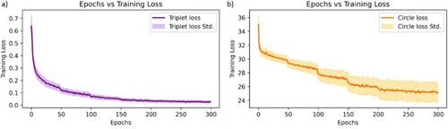
The graphical representation of loss values over 300 training epochs, as depicted in Figure 10 and its corresponding figures, compellingly demonstrates that both CNN-3 and CNN-4 have effectively grasped the underlying data distributions pertaining to multivariate data. Notably, a distinct pattern emerges from the loss curves. In the case of CNN-3, which utilises the triplet loss function (as shown in Figure 10(a)), it’s evident that the loss curve levels off around the 150-epoch mark. This levelling indicates that the model has proficiently captured the essential data features and representations, with no significant performance improvements observed beyond this point. Conversely, the CNN-4 model, employing the circle loss (as illustrated in Figure 10(b)), follows a similar pattern but reaches a saturation point at around 200 epochs. This specific trend in the loss values suggests that CNN-4 continues to refine its representations and enhance its feature extraction capabilities up to this juncture. These insights shed light on the convergence behaviour of both models. While CNN-3 achieves stability relatively early in the training process, CNN-4 consistently improves its performance over a somewhat extended training duration. The subtle differences in the convergence patterns highlight the unique attributes of the triplet and circle loss functions, stressing the significance of choosing the appropriate loss function that aligns with the learning goals and dataset attributes. Additionally, the variation in training loss values depicted in Figure 10 originates from the distinct implementations of their respective loss functions. Whereas the triplet loss function focuses on enforcing margins for discriminative features, the circle loss function prioritises reducing inter-class variance and minimising intra-class variance, leading to divergent optimisation dynamics.

Figure 10. Learning curves illustrating model training progress: (a) Evaluating performance and convergence of the CNN-3 model using Triplet loss (b) Evaluating performance and convergence of the CNN-4 model using circle loss

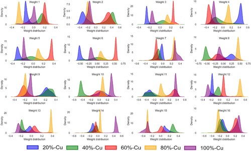
An additional technique utilised to evaluate the effectiveness of our trained CNN models involves visualising their lower-dimensional representations, specifically the 1 × 16 feature maps extracted from the last fully connected layer. In Figure 11, we present distribution plots highlighting the weights originating from sixteen specific nodes within the last fully connected layer of the CNN-3 model, which was trained using the validation dataset. This visualisation reveals distinct and well-defined distributions, each corresponding to one of the five distinct composition grades under consideration. The clear separation of these clusters within the feature space confirms the model's ability to discern subtle patterns and features indicative of the various build grades. Such visualisations serve as a potent method to qualitatively validate the learned representations and underscore the model's capacity to capture and differentiate between the underlying characteristics of the data classes, ultimately reinforcing the model's effectiveness and reliability.

Figure 11. Distribution of latent space representations obtained from CNN-3 trained with triplet loss, applied to sensor fusion signals combining acoustic and optical datastreams.

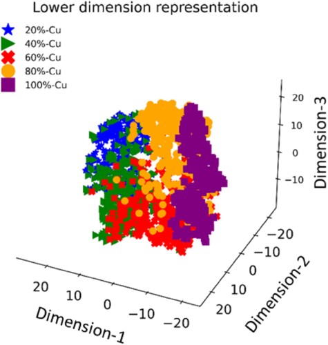
An alternative method for evaluating the performance of the trained CNN-4 model involves visualising its lower-dimensional representations, specifically the feature maps obtained from the final fully connected layer when applied to the multivariate acoustic and photodiode data. In Figure 12, we present a compelling 3D visualisation of these lower-dimensional representations generated by the output from the last fully connected layer of the CNN-4 model. These representations were computed using t-distributed stochastic neighbour embedding (t-SNE), with a perplexity value set at 20. This visualisation reveals distinct clusters, each corresponding to one of the five distinct composition grades. The well-separated clusters within the feature space provide compelling evidence that the model has successfully learned to differentiate between the various build grades using the multivariate acoustic and photodiode data.

Figure 12. Distribution of lower-dimensional representations obtained from CNN-4 trained with circle loss, applied to sensor fusion signals combining acoustic and optical data streams.

The feature map visualisations obtained from both CNN-3 and CNN-4 models, revealing clear evidence of clustering, offer an exciting opportunity to be effectively employed in conjunction with traditional classifiers to assess how contrastive learners excel at extracting features that traditional classification learners struggle with, especially in data spaces characterised by soft margins, as is the case with composition monitoring. The integration of contrastive learning techniques with traditional classification methods could potentially lead to enhanced performance and the ability to discern subtle patterns and distinctions that may have been challenging to capture using conventional approaches in such complex data environments. This intriguing exploration will be further investigated in the next section.

5.1. XGBoost – ensemble learning

Ensemble learning is a powerful technique used in ML to mitigate two common challenges in building predictive models: bias and variance [75]. These challenges arise when working with individual models, as they can either be too simplistic and biased or overly complex and prone to overfitting the training data. Ensemble learning aims to strike a balance by combining the predictions of multiple individual models. XGBoost (eXtreme Gradient Boosting) is an example of an ensemble model that utilises boosting and decision trees [76]. It excels in classification and regression tasks and is known for scalability. XGBoost incrementally builds an ensemble of weaker models like decision trees, optimising a differentiable loss function to enhance generalisation and reduce overfitting. It offers advantages like speed compared to AdaBoost, effective regularisation, and features subsampling similar to random forests. However, it's more complex to understand, visualise, and fine-tune than AdaBoost and random forests, with numerous adjustable hyperparameters to improve performance.

The feature representations generated by trained CNN-3 and CNN-4, utilising the contrastive learning methods discussed earlier, combine to form a crucial dataset. This dataset is instrumental in the training and fine-tuning of the XGBoost classifier. We employed the feature maps generated by both CNNs to create separate feature spaces for training two XGBoost classifiers, XG-1 and XG-2. In training these classifiers, we followed the standard practice of randomly splitting the datasets with known ground truth into 70% for training and 30% for testing. Our primary objective is to achieve precise classification across five different compositions. The entire implementation was conducted using Python's scikit-learn libraries [77]. To optimise the performance of the XGBoost Classifier, we fine-tuned the hyperparameters according to the configurations outlined in Table 8.

Table 8. XGBoost classifier training parameters.

Parameters	XG Boost
Learning rate	0.3
Tree_method	auto
Depth	6
Sampling method	uniform
gamma	0.1
subsample	1
colsample_bytree	1
Objective	classification
Validation method	Stratifiedfold cross-validation

The performance of the two XGBoost models was assessed using stratified-fold cross-validation, and the results are summarised in Table 9, which includes a confusion matrix to showcase predictive accuracy and errors. The overall prediction accuracy for both XGBoost models was impressive, with 94.2% and 97.6%. The key takeaway from these results is that XGBoost-based classifiers present a highly promising approach for monitoring tasks when combined with feature representations generated using contrastive learning methods. Notably, they outperform traditional classifiers in this context. Traditional classifiers often face challenges when dealing with data spaces characterised by soft margins, where the decision boundaries between different classes are not well-defined.

Table 9. Table shows accuracies for predicted label (wear classes) vs true label (ground truth) on five classes.

	Ground truth
Classification (accuracy [%])	20%-Cu	40%-Cu	60%-Cu	80%-Cu	100%-Cu
20%-Cu	92	7	0	1	0
	97	3	0	0	0
40%-Cu	7	90	3	1	0
	2	97	1	0	0
60%-Cu	0	2	94	3	0
	0	1	97	2	0
80%-Cu	0	0	4	95	0
	0	0	0	97	0
100%-Cu	0	0	0	0	100
	0	0	0	0	100

Tables for the classification accuracy results using the two XGBoost classifier models (XGBoost-1 and XGBoost-2). The classification results in each cell from top to bottom are for: XGBoost-1 and XGBoost-2. All values are in %.

The improved accuracy observed with XG-2 in conjunction with CNN-4, which was trained using circle loss, can be attributed to the regularisation impact introduced by circle loss during CNN-4's training process. This regularisation effect enhances feature representations’ quality. Relying solely on a single monitoring solution, such as a photodiode tracking melt pool intensity or air-borne AE, proves insufficient for accurately assessing process stability or detecting flaws, particularly in routine LPBF process monitoring involving multi-materials. Our research adopts a data fusion approach to tackle this challenge and enhance compositional monitoring performance. Our methodology incorporates multiple sensor modalities, including acoustic and optical intensities in the laser wavelength spectrum. Specifically, our work explores the challenges associated with monitoring multi-material deposition, particularly in materials such as copper that exhibit high reflectivity to infrared wavelengths when combined with stainless steel. This aspect presents a novel and significant challenge, which we aim to address through data-driven approaches and optimisation of sensor fusion techniques. This paper builds upon existing research by integrating data fusion techniques, facilitating the exchange of complementary information among these sensors and thereby enhancing their correlation with actual flaws in compositional monitoring. This advancement lays the groundwork for achieving high confidence in quality control in future LPBF applications involving multi-materials.

6. Conclusion

In conclusion, our research has delved into the intricate analysis of AE signals and optical emissions concerning laser wavelength in monitoring LPBF processes across diverse materials. By meticulously examining five distinct powder compositions and utilising a specialised monitoring system integrated into a commercial LPBF machine, we have gained profound insights into the interplay among powder composition, AE signals, and optical emissions. We have effectively categorised signals associated with various powder compositions by employing methodologies rooted in contrastive deep learning. As we reflect on the outcomes, several overarching conclusions become apparent:

• The segmentation of AE waveform signals into fifteen frequency bands revealed pronounced variations in energy levels among the five powder compositions, indicating distinct melt pool dynamics. A clear correlation emerged between the intensity of optical signals at the laser wavelength and the powder composition, even under identical process parameters.

• Our exploration of supervised classification using a Convolutional Neural Network (CNN) on photodiode signals and acoustic data highlighted the superiority of a strategy that fused both types of information, resulting in enhanced prediction accuracy.

• Integrating a contrastive learner with a sensor fusion strategy has emerged as a valuable approach for monitoring LPBF processes across multiple materials. Visualisation of the lower-level embedded space of CNN models trained using contrastive loss functions revealed coherent groupings of multivariate data streams corresponding to the five compositions based on their similarities.

• Despite subtle architectural differences among the CNNs, compelling evidence supports the utilisation of contrastive learners for the monitoring task in multi-material scenarios. The higher accuracy demonstrates this attained when employing learned representations from CNN-3&4 as input for XGBoost-based classification, compared to conventional CNN (CNN-1&2) training.

Furthermore, our future research endeavours will focus on testing the robustness of our methodology under challenging conditions involving varying LPBF regimes. We aim to validate the efficacy of our proposed strategy across different scan lengths, thereby examining various time scales comprehensively. Additionally, efforts will be directed towards refining CNN architectures, optimising network weights, and determining suitable weights for the loss function to enhance training efficacy. Furthermore, our ongoing research examines the compositions of melt pools and plumes using multispectral imaging. We aim to seamlessly continue our current research efforts while recognising the potential for further advancement by integrating physics-informed models with machine learning techniques. Acknowledging the significance of mechanistic understanding in propelling the field forward, we plan to delve into this aspect in our future research endeavours. For those interested, the data and codes for this study can be accessed in the following repository (https://c4science.ch/diffusion/12999/).

Data availability statement

The data on the findings in this study are available in the repo (https://c4science.ch/diffusion/12999/) and will be available online after the publication of the manuscript.

Disclosure statement

No potential conflict of interest was reported by the author(s).

Additional information

Funding

The authors would like to acknowledge the financial support of the project Multi-Mat from the Strategic Focus Area Advanced Manufacturing (SFA-AM) programme, a strategic initiative of the ETH Board. The authors would like to thank Xiaoshuang Li for contributing to the process space optimisation.

References

- Ahmed N, Barsoum I, Haidemenopoulos G, et al. Process parameter selection and optimization of laser powder bed fusion for 316L stainless steel: A review (in English). J Manuf Process. 2022;75:415–434. doi:10.1016/j.jmapro.2021.12.064
- Sanchez-Mata O, Wang X, Muniz-Lerma JA, et al. Dependence of mechanical properties on crystallographic orientation in nickel-based superalloy Hastelloy X fabricated by laser powder bed fusion. J Alloys Compd. 2021;865:158868. doi:10.1016/j.jallcom.2021.158868
- Wang L, Song Z, Zhang X, et al. Developing ductile and isotropic Ti alloy with tailored composition for laser powder bed fusion. Addit Manuf. 2022;52:102656. doi:10.1016/j.addma.2022.102656
- Rometsch PA, Zhu Y, Wu X, et al. Review of high-strength aluminium alloys for additive manufacturing by laser powder bed fusion. Mater Des. 2022;219:110779. doi:10.1016/j.matdes.2022.110779
- Zhou W, Kousaka T, Moriya S-i, et al. Fabrication of a strong and ductile CuCrZr alloy using laser powder bed fusion. Addit Manuf Lett. 2023;5:100121. doi:10.1016/j.addlet.2023.100121
- Zhang X, Pan T, Chen Y, et al. Additive manufacturing of copper-stainless steel hybrid components using laser-aided directed energy deposition. J Mater Sci Technol. 2021;80:100–116. doi:10.1016/j.jmst.2020.11.048
- Chen J, Yang Y, Song C, et al. Interfacial microstructure and mechanical properties of 316L/CuSn10 multi-material bimetallic structure fabricated by selective laser melting. Mater Sci Eng A. 2019;752:75–85. doi:10.1016/j.msea.2019.02.097
- Rodrigues TA, Bairrão N, Farias FWC, et al. Steel-copper functionally graded material produced by twin-wire and arc additive manufacturing (T-WAAM). Mater Des. 2022;213:110270. doi:10.1016/j.matdes.2021.110270
- Leedy KD, Stubbins JF. Copper alloy–stainless steel bonded laminates for fusion reactor applications: crack growth and fatigue. Mat Sci Eng a-Struct. 2001;297(1-2):19–25. doi:10.1016/S0921-5093(00)01274-0
- Wang S, Ning J, Zhu L, et al. Role of porosity defects in metal 3D printing: formation mechanisms, impacts on properties and mitigation strategies. Mater Today. 2022;59:133–160. doi:10.1016/j.mattod.2022.08.014
- Du Plessis A, Yadroitsava I, Yadroitsev I. Effects of defects on mechanical properties in metal additive manufacturing: A review focusing on X-ray tomography insights. Mater Des. 2020;187:108385. doi:10.1016/j.matdes.2019.108385
- Cerniglia D, Scafidi M, Pantano A, et al. Inspection of additive-manufactured layered components. Ultrasonics. 2015;62:292–298. doi:10.1016/j.ultras.2015.06.001
- Acevedo R, Sedlak P, Kolman R, et al. Residual stress analysis of additive manufacturing of metallic parts using ultrasonic waves: state of the art review. J Mater Res Technol. 2020;9(4):9457–9477. doi:10.1016/j.jmrt.2020.05.092
- Shah P, Racasan R, Bills P. Comparison of different additive manufacturing methods using computed tomography. Case Stud Nondestr Test Eval. 2016;6:69–78. doi:10.1016/j.csndt.2016.05.008
- Tammas-Williams S, Withers PJ, Todd I, et al. The influence of porosity on fatigue crack initiation in additively manufactured titanium components. Sci Rep. 2017;7(1):7308. doi:10.1038/s41598-017-06504-5
- Mazumder J. Design for metallic additive manufacturing machine with capability for “Certify as You Build”. Procedia CIRP. 2015;36:187–192. doi:10.1016/j.procir.2015.01.009
- Zhu L, Xue P, Lan Q, et al. Recent research and development status of laser cladding: A review. Opt Laser Technol. 2021;138:106915. doi:10.1016/j.optlastec.2021.106915
- Wang C, Tan X, Tor SB, et al. Machine learning in additive manufacturing: State-of-the-art and perspectives. Addit Manuf. 2020;36:101538. doi:10.1016/j.addma.2020.101538
- Seifi M, Gorelik M, Waller J, et al. Progress towards metal additive manufacturing standardization to support qualification and certification. JOM. 2017;69:439–455. doi:10.1007/s11837-017-2265-2
- Everton SK, Hirsch M, Stravroulakis P, et al. Review of in-situ process monitoring and in-situ metrology for metal additive manufacturing. Mater Des. 2016;95:431–445. doi:10.1016/j.matdes.2016.01.099
- Hossain MS, Taheri H. In situ process monitoring for additive manufacturing through acoustic techniques. J Mater Eng Perform. 2020;29(10):6249–6262. doi:10.1007/s11665-020-05125-w
- Lane B, Grantham S, Yeung H, et al. Performance characterization of process monitoring sensors on the NIST additive manufacturing metrology testbed. 2017 International solid freeform fabrication symposium. University of Texas at Austin; 2017. https://api.semanticscholar.org/CorpusID:55777435.
- Montazeri M, Rao P. Sensor-based build condition monitoring in laser powder bed fusion additive manufacturing process using a spectral graph theoretic approach. J Manuf Sci Eng. 2018;140(9):091002. doi:10.1115/1.4040264
- Pandiyan V. Deep learning-based monitoring of laser powder bed fusion process on variable time-scales using heterogeneous sensing and operando X-ray radiography guidance. Addit Manuf. 2022;58:103007. doi:10.1016/j.addma.2022.103007
- Özel T, Shaurya A, Altay A, et al. Process monitoring of meltpool and spatter for temporal-spatial modeling of laser powder bed fusion process. Procedia CIRP. 2018;74:102–106. doi:10.1016/j.procir.2018.08.049
- Pandiyan V, Wróbel R, Leinenbach C, et al. Optimizing in-situ monitoring for laser powder bed fusion process: deciphering acoustic emission and sensor sensitivity with explainable machine learning. J Mater Process Technol. 2023: 118144. doi:10.1016/j.jmatprotec.2023.118144
- Pandiyan V, Drissi-Daoudi R, Shevchik S, et al. Analysis of time, frequency and time-frequency domain features from acoustic emissions during Laser Powder-Bed fusion process. Procedia CIRP. 2020;94:392–397. doi:10.1016/j.procir.2020.09.152
- Imani F, Gaikwad A, Montazeri M, et al. Process mapping and in-process monitoring of porosity in laser powder bed fusion using layerwise optical imaging. J Manuf Sci Eng. 2018;140(10):101009. doi:10.1115/1.4040615
- McCann R, Obeidi MA, Hughes C, et al. In-situ sensing, process monitoring and machine control in Laser Powder Bed Fusion: A review. Addit Manuf. 2021;45:102058. doi:10.1016/j.addma.2021.102058
- Taherkhani K, Ero O, Liravi F, et al. On the application of in-situ monitoring systems and machine learning algorithms for developing quality assurance platforms in laser powder bed fusion: A review. J Manuf Process. 2023;99:848–897. doi:10.1016/j.jmapro.2023.05.048
- Cai Y, Xiong J, Chen H, et al. A review of in-situ monitoring and process control system in metal-based laser additive manufacturing. J Manuf Syst. 2023;70:309–326. doi:10.1016/j.jmsy.2023.07.018
- Lane B, Zhirnov I, Mekhontsev S, et al. Transient laser energy absorption, co-axial melt pool monitoring, and relationship to melt pool morphology. Addit Manuf. 2020;36:101504. doi:10.1016/j.addma.2020.101504
- Schwerz C, Nyborg L. Linking in situ melt pool monitoring to melt pool size distributions and internal flaws in laser powder bed fusion. Metals (Basel). 2021;11(11):1856. doi:10.3390/met11111856
- Khanzadeh M, Tian W, Yadollahi A, et al. Dual process monitoring of metal-based additive manufacturing using tensor decomposition of thermal image streams. Addit Manuf. 2018;23:443–456. doi:10.1016/j.addma.2018.08.014
- Bertoli US, Guss G, Wu S, et al. In-situ characterization of laser-powder interaction and cooling rates through high-speed imaging of powder bed fusion additive manufacturing. Mater Des. 2017;135:385–396. doi:10.1016/j.matdes.2017.09.044
- Yang Z, Zhu L, Wang S, et al. Effects of ultrasound on multilayer forming mechanism of Inconel 718 in directed energy deposition. Addit Manuf. 2021;48:102462. doi:10.1016/j.addma.2021.102462
- Ashby A, Guss G, Ganeriwala RK, et al. Thermal history and high-speed optical imaging of overhang structures during laser powder bed fusion: A computational and experimental analysis. Addit Manuf. 2022;53:102669. doi:10.1016/j.addma.2022.102669
- Forien J-B, Calta NP, DePond PJ, et al. Detecting keyhole pore defects and monitoring process signatures during laser powder bed fusion: A correlation between in situ pyrometry and ex situ X-ray radiography. Addit Manuf. 2020;35:101336. doi:10.1016/j.addma.2020.101336
- Gutknecht K, Cloots M, Wegener K. Relevance of single channel signals for two-colour pyrometer process monitoring of laser powder bed fusion. Int J Mechatron Manuf Syst. 2021;14(2):111–127. doi:10.1504/IJMMS.2021.119152
- Vallabh CKP, Zhao X. Melt pool temperature measurement and monitoring during laser powder bed fusion based additive manufacturing via single-camera two-wavelength imaging pyrometry (STWIP). J Manuf Process. 2022;79:486–500. doi:10.1016/j.jmapro.2022.04.058
- Mao Z, Feng W, Ma H, et al. Continuous online flaws detection with photodiode signal and melt pool temperature based on deep learning in laser powder bed fusion. Opt Laser Technol. 2023;158:108877. doi:10.1016/j.optlastec.2022.108877
- Mitchell JA, Ivanoff TA, Dagel D, et al. Linking pyrometry to porosity in additively manufactured metals. Addit Manuf. 2020;31:100946. doi:10.1016/j.addma.2019.100946
- Lapointe S, Guss G, Reese Z, et al. Photodiode-based machine learning for optimization of laser powder bed fusion parameters in complex geometries. Addit Manuf. 2022;53:102687. doi:10.1016/j.addma.2022.102687
- Khairallah SA, Anderson AT, Rubenchik A, et al. Laser powder-bed fusion additive manufacturing: physics of complex melt flow and formation mechanisms of pores, spatter, and denudation zones. Acta Mater. 2016;108:36–45. doi:10.1016/j.actamat.2016.02.014
- Fisher BA, Lane B, Yeung H, et al. Toward determining melt pool quality metrics via coaxial monitoring in laser powder bed fusion. Manuf Lett. 2018;15:119–121. doi:10.1016/j.mfglet.2018.02.009
- Zhao C, et al. Real-time monitoring of laser powder bed fusion process using high-speed X-ray imaging and diffraction. Sci Rep. 2017;7(1):1–11. doi:10.1038/s41598-016-0028-x
- Mazzoleni L, Demir AG, Caprio L, et al. Real-time observation of melt pool in selective laser melting: spatial, temporal, and wavelength resolution criteria. IEEE Trans Instrum Meas. 2020;69(4):1179–1190. doi:10.1109/TIM.2019.2912236
- Drissi-Daoudi R, Pandiyan V, Logé R, et al. Differentiation of materials and laser powder bed fusion processing regimes from airborne acoustic emission combined with machine learning. Virtual Phys Prototyp. 2022;17(2):181–204. doi:10.1080/17452759.2022.2028380
- Gaikwad A, Williams RJ, de Winton H, et al. Multi phenomena melt pool sensor data fusion for enhanced process monitoring of laser powder bed fusion additive manufacturing. Mater Des. 2022;221:110919. doi:10.1016/j.matdes.2022.110919
- Khanzadeh M, Chowdhury S, Marufuzzaman M, et al. Porosity prediction: supervised-learning of thermal history for direct laser deposition. J Manuf Syst. 2018;47:69–82. doi:10.1016/j.jmsy.2018.04.001
- Ye D, Fuh Y, Zhang Y, et al. Defects recognition in selective laser melting with acoustic signals by SVM based on feature reduction. IOP Conf Ser: Mater Sci Eng. 2018;436(1):012020. doi:10.1088/1757-899X/436/1/012020
- Ye D, Hong GS, Zhang Y, et al. Defect detection in selective laser melting technology by acoustic signals with deep belief networks. Int J Adv Manuf Technol. 2018;96:2791–2801. doi:10.1007/s00170-018-1728-0
- Pandiyan V, Drissi-Daoudi R, Shevchik S, et al. Semi-supervised monitoring of laser powder bed fusion process based on acoustic emissions. Virtual Phys Prototyp. 2021;16(4):481–497. doi:10.1080/17452759.2021.1966166
- Shevchik SA, Kenel C, Leinenbach C, et al. Acoustic emission for in situ quality monitoring in additive manufacturing using spectral convolutional neural networks. Addit Manuf. 2018;21:598–604. doi:10.1016/j.addma.2017.11.012
- Becker P, Roth C, Rönnau A, et al. Porosity detection in powder bed fusion additive manufacturing with convolutional neural networks. doi: 10.18178/wcse.2022.04.117.
- Pandiyan V, Drissi-Daoudi R, Shevchik S, et al. Deep transfer learning of additive manufacturing mechanisms across materials in metal-based laser powder bed fusion process. J Mater Process Technol. 2022;303:117531. doi:10.1016/j.jmatprotec.2022.117531
- Shevchik SA, Masinelli G, Kenel C, et al. Deep learning for in situ and real-time quality monitoring in additive manufacturing using acoustic emission. IEEE Trans Ind Inf. 2019;15(9):5194–5203. doi:10.1109/TII.2019.2910524
- Xing W, Chu X, Lyu T, et al. Using convolutional neural networks to classify melt pools in a pulsed selective laser melting process. J Manuf Process. 2022;74:486–499. doi:10.1016/j.jmapro.2021.12.030
- Kwon O, Kim HG, Ham MJ, et al. A deep neural network for classification of melt-pool images in metal additive manufacturing. J Intell Manuf. 2020;31:375–386. doi:10.1007/s10845-018-1451-6
- Pandiyan V, Wróbel R, Richter RA, et al. Monitoring of Laser Powder Bed Fusion process by bridging dissimilar process maps using deep learning-based domain adaptation on acoustic emissions. Addit Manuf. 2024: 103974. doi:10.1016/j.addma.2024.103974
- Pandiyan V, Wróbel R, Richter RA, et al. Self-Supervised Bayesian representation learning of acoustic emissions from laser powder bed Fusion process for in-situ monitoring. Mater Des. 2023;235:112458. doi:10.1016/j.matdes.2023.112458
- Khosla P, et al. Supervised contrastive learning. Adv Neural Inf Process Syst. 2020;33:18661–18673. doi:10.48550/arXiv.2004.11362
- Chen T, Kornblith S, Norouzi M, et al. A simple framework for contrastive learning of visual representations. International Conference on Machine Learning. 2020;2020: PMLR:1597–1607. doi:10.48550/arXiv.2002.05709
- Spijkervet J, Burgoyne JA. Contrastive learning of musical representations. arXiv preprint arXiv:2103.09410; 2021. doi: 10.48550/arXiv.2103.09410.
- Pandiyan V, Cui D, Le-Quang T, et al. In situ quality monitoring in direct energy deposition process using co-axial process zone imaging and deep contrastive learning. J Manuf Process. 2022;81:1064–1075. doi:10.1016/j.jmapro.2022.07.033
- Ge W. Deep metric learning with hierarchical triplet loss. Proceedings of the European Conference on Computer Vision (ECCV); 2018. p. 269–285. doi:10.48550/arXiv.1810.06951
- Dong X, Shen J. Triplet loss in siamese network for object tracking. Proceedings of the European Conference on Computer Vision (ECCV); 2018. p. 472–488. doi:10.1007/978-3-030-01261-8_28
- Sun Y, et al. Circle loss: A unified perspective of pair similarity optimization. Proceedings of the IEEE/CVF Conference on Computer Vision and Pattern Recognition; 2020. p. 6398–6407. doi:10.48550/arXiv.2002.10857
- Xiao R. Adaptive margin circle loss for speaker verification. arXiv preprint arXiv:2106.08004; 2021. doi:10.48550/arXiv.2106.08004
- Li J, Cai Y, Yan F, et al. Porosity and liquation cracking of dissimilar Nd: YAG laser welding of SUS304 stainless steel to T2 copper. Opt Laser Technol. 2020;122:105881. doi:10.1016/j.optlastec.2019.105881
- Xiao P, Wang L, Tang Y, et al. Effect of wire composition on microstructure and penetration crack of laser-cold metal transfer hybrid welded Cu and stainless steel joints. Mater Chem Phys. 2023;299:127480. doi:10.1016/j.matchemphys.2023.127480
- Gao Z, Yang Y, Wang L, et al. Formation mechanism and control of solidification cracking in laser-welded joints of steel/copper dissimilar metals. Metals (Basel). 2022;12(7):1147. doi:10.3390/met12071147
- Chen S, Yu X, Huang J, et al. Interfacial ferrite band formation to suppress intergranular liquid copper penetration of solid steel. J Alloys Compd. 2019;773:719–729. doi:10.1016/j.jallcom.2018.09.282
- Paszke A, et al. Pytorch: An imperative style, high-performance deep learning library. Adv Neural Inf Process Syst. 2019: 8026–8037. doi:10.48550/arXiv.1912.01703
- Zhou Z-H, Zhou Z-H. Ensemble learning. Singapore: Springer; 2021. doi:10.1007/978-0-387-73003-5_293
- Chen T, He T, Benesty M, et al. Xgboost: Extreme Gradient Boosting. R package version 0.4-2 1, 2015; (4):1–4.
- Pedregosa F, Varoquaux G, Gramfort A, et al. Scikit-Learn: Machine Learning in Python. J Mach Learn Res. 2011; 12: 2825–2830.