A semi-analytical approach to wire arc additive manufacturing simulation for deposition sequence optimisation

ABSTRACT

Categorised as a directed energy deposition process, wire arc additive manufacturing (WAAM) is a promising technology for fabricating large-scale structures and components across various industries. However, the quality of WAAM parts depends on the tool trajectory, as it affects the temperature distribution. Ideally, temperature-related issues, such as overheating, are minimised by choosing an optimal deposition sequence. Selecting the deposition sequence solely on intuition is an unreliable approach, particularly when dealing with complex and irregular parts. This paper introduces a simplified WAAM simulation (SWS) model, which was embedded into an optimisation procedure for determining the optimal deposition sequence of thin-walled WAAM parts. The proposed method is based on a semi-analytical function, which was calibrated and validated using thermal histories obtained from finite element simulations. The findings showed that the proposed SWS model can reproduce the average thermal history at predefined positions within a sample part with minimal computational effort. Moreover, the optimisation successfully identified optimal deposition sequences for producing the sample part regarding a given optimisation criterion. The outcomes of this research contribute to the tool trajectory planning process for WAAM parts. An optimal deposition sequence improves WAAM part quality, increasing the usability of WAAM technology in the production industry.

KEYWORDS:

• Directed energy deposition
• model simplification
• deposition sequence
• tool trajectory
• thermal simulation
• optimisation

Introduction

Wire arc additive manufacturing (WAAM) is an additive manufacturing (AM) technology for the near-net-shape manufacturing of large-scale parts in a variety of industries [1]. This technology involves the controlled deposition and stacking of weld seams into a three-dimensional geometry, employing gas-tungsten, gas-metal, or plasma-arc welding processes [2]. Compared to other AM processes, WAAM stands out with its fast build-up rates, large build volumes, and low initial investments [3]. With these attributes, WAAM is particularly suited for producing thin-walled and large-volume components [4, 5].

However, some challenges still need to be addressed for a large-scale industrial adoption of WAAM. Due to the high heat input into the part during the welding process, components manufactured using WAAM are prone to temperature-related defects, such as micro-cracking [6, 7], porosity [8], residual stresses [9], and shape distortion [10, 11]. Especially excessive heat and material accumulation, often observed in corners or wall joint sections of the components, can lead to unintended structural collapse [12], resulting in the production of scrap parts.

One approach for reducing these unwanted thermal effects and to maintain consistent quality across all layers is to ensure a low, homogeneous, and reproducible surface temperature on the top layer before the deposition of the next layer is initiated. Therefore, it is common practice to let the part cool down after the deposition of each layer until it reaches a specified temperature, which is referred to as the interpass or interlayer temperature. While the interpass temperature is usually defined between layers in build-direction, its relevance extends to single layers as well, when the welding torch revisits specific areas of the structure within a single layer. Control of the interpass temperature can be accomplished, for instance, by active cooling [10, 13] or by incorporating a certain interlayer dwell time [14]. The positive effects of the dwell time on the properties of the final WAAM part have been addressed extensively in previous studies and include the improvement of mechanical and geometrical properties of the part [14, 15]. However, increasing the dwell time inherently extends the manufacturing time for the part, consequently reducing productivity.

An approach circumventing this drawback is implementing path planning strategies. The strong influence of the deposition sequence on the distortion of a substrate plate was shown using experimental methods [16] as well as finite element (FE) simulations [11, 17]. The utilisation of simulations for path planning is advantageous since a validated simulation model enables the exploration of numerous potential paths without the logistical complexities and costs associated with conducting and evaluating physical experiments. Presently, thermomechanical FE simulations offer the capability to predict the temperature and distortion of WAAM parts for a designated path in the simulation [18, 19]. However, these simulations demand significant computer processing time. Given the countless possibilities for deposition sequences in a path planning task, simulating all, or even a fraction of them, becomes impractical. Traditional FE methods can only handle a limited number of sequences due to the time-intensive nature of the simulation. Consequently, a need for simplified models arises that can approximate the WAAM process swiftly, enabling the evaluation of numerous deposition sequences. Although these models entail precision compromises due to simplifications, their primary objective is characterised by a qualitative result comparison rather than an absolute accuracy.

In literature, such attempts have been made with varying objectives. Aiming for a homogeneous temperature distribution in the WAAM part, an analytical model was formulated, considering one-dimensional heat conduction and radiation [20]. The temporal discretisation of this model was implemented using the finite difference method, which encompasses solving a system of equations in each time step, leading to moderate computational effort. In another study, the best and the worst welding sequences for a pipe girth weld with regard to minimal distortions were identified using an optimisation procedure and a surrogate model [21]. However, this surrogate model is exclusively applicable to the specific problem of the pipe geometry and is not directly transferable to other parts. Another simplified simulation facilitated the fast evaluation of deposition sequences for thin-walled WAAM parts [22]. This model was employed to compare four different deposition sequences with regard to robot kinematics and temperature homogeneity. However, the model was not integrated in an optimisation workflow.

Several endeavours were undertaken within the field of deposition sequence optimisation employing simplified models for WAAM. Nevertheless, a research gap exists in the absence of a model characterised by a very high computational efficiency, the adaptability to different geometries, and the suitability for optimisation.

This paper addresses these aspects by introducing the simplified WAAM simulation (SWS), a novel, semi-analytical model for the thermal simulation of the WAAM process with a focus on thin-walled parts. Compared to the existing body of research, the SWS provides the following advantages:

• It is computationally efficient.

• It can be used to simulate different thin-walled geometries.

• It can be integrated into a deposition sequence optimisation procedure.

The SWS in combination with a deposition sequence optimisation could be integrated into the WAAM workflow as a tool supporting the path planning process. The long-term industrial benefits lie in the enhancement of the productivity of the the WAAM process. Simulating and optimising the deposition sequence with thermal criteria before the WAAM process results in a reduction of fabricated scrap parts, ultimately lowering overall production costs and facilitating a more wide-spread implementation of WAAM in the production industry.

This paper functions as a proof of concept for the SWS and its implementation into an optimisation procedure. The maximum interpass temperature was chosen as the optimisation criterion. The objective of this paper is to demonstrate the following:

• With the SWS, it is possible to efficiently predict thermal histories at specific locations within the part with sufficient accuracy.

• The maximum interpass temperature can be effectively minimised by combining the SWS with an optimisation procedure.

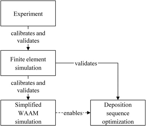
The subsequent sections of this paper are structured as follows. Firstly, the mathematical foundation of the model, rooted in analytical cooling functions, is explained. Secondly, the two-step calibration and validation procedure of the model is elucidated. For this process, an FE model is experimentally calibrated and validated. Then, the validated FE model is in turn used to calibrate and validate the SWS model. Subsequently, the SWS model is integrated in an optimisation procedure. In this procedure, the SWS is executed for all possible deposition sequences of an exemplary part and the results are assessed with the objective of minimising the maximum interpass temperature. This optimisation aims at reducing the risk of overheating and thus improving the process stability and the quality of the final part. Finally, the results are presented and discussed.

Proposed model

Principle

The terms ‘node’, ‘vertex’, and ‘edge’ are commonly used in both the context of the finite element analysis (FEA) and graph theory [23, 24]. To ensure clarity in the context of this paper, the term ‘node’ exclusively refers to the FEA, while the terms ‘vertex’ and ‘edge’ are only associated with the graph theory.

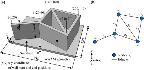
In the proposed model, a thin-walled WAAM part is represented as a mathematical graph. Figure 1 illustrates the example part, a kite geometry, in both its three-dimensional computer-aided design (CAD) form in Figure 1(a) and its corresponding mathematical graph form in Figure 1(b). This geometry was chosen due to its non-Eulerian and non-symmetrical nature. It is intended to represent an arbitrary but nonetheless feasible geometry for a thin-walled WAAM part, thereby serving as a proof of concept for both the SWS and the optimisation of the deposition sequence. As visualised, the thin-walled structure in its graph representation consists of five vertices ${\mathrm{v}}_i$ and six edges ${\mathrm{e}}_j$. The vertices were placed at the wall joint positions of the part, while the edges ${\mathrm{e}}_j$ represent the walls of the part.

Figure 1. The example part, a kite geometry, as (a) three-dimensional CAD part and (b) as mathematical graph; z is the build-direction; all measurements and coordinates are given in mm.

Figure 2(a) shows the working principle of the proposed SWS. Each two vertices connected via an edge represent a welding operation. The simulated welding torch begins a welding operation at a vertex and moves along an adjacent edge until it reaches the next vertex. If the next vertex is linked to further vertices by corresponding edges, the welding torch may proceed further to the next vertex, continuing the welding operation. Alternatively, the welding is stopped if the welding torch is instructed to, or if the connected vertex is not linked to any further vertices. Thus, the vertices ${\mathrm{v}}_i$ represent potential start and end points for welding operations. Once a welding operation concludes, the welding torch traverses to another vertex and initiates the next welding operation. During a non-welding traverse operation, the path is not constrained to follow the edges. Consequently, the welding torch can proceed to its destination in the shortest possible path, which is a straight line. The corresponding user-set velocities of the welding torch determine the durations for welding and non-welding traverse operations. The simulation of a single layer entails performing welding operations on all the edges exactly once, while the simulation of multiple layers requires the same welding and non-welding traverse operations to be executed multiple times.

Figure 2. (a) Demonstrations of the working principle of the SWS using an example part; (b) qualitative temperature history at the nodes of the example part over two consecutive layers; z is the build-direction.

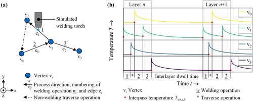
At the start of the simulation, all vertices are assigned an initial temperature. Each time a vertex is reached in a welding operation, a predetermined amount of energy is supplied to the vertex, which immediately raises the vertex temperature. The subsequent cooling behaviour of the vertex is calculated using a semi-analytical cooling function. Owing to the analytical nature of the temperature history, intermediate time steps are not required. The simulation result of the SWS consists of the thermal histories across all the vertices of a part, as qualitatively shown in Figure 2(b) for the example part in Figure 2(a), spanning two consecutive layers. The interpass temperature $T_{\mathrm{int},i,k}$ is calculated infinitesimally just before the welding torch arrives at a vertex ${\mathrm{v}}_i$ for the $k$-th time and the temperature is increased. In comparison to the results obtained from a FE simulation, the SWS only provides thermal histories at the specific vertices defined within the part, rather than across the entire domain.

The presented SWS model is a thermal model subject to the following model simplifications:

• Heat conduction predominantly occurs along the walls and towards the substrate.

• The density $\rho$, the specific heat capacity $c_{\mathrm{p}}$ and the thermal conductivity $\lambda$ of the used material are assumed constant.

• The effects of phase transformations are neglected.

Moreover, the presented SWS model operates under the following assumptions regarding the deposition process:

• Welding and non-welding traverse operations are restricted to starting and ending at vertices.

• Both welding and non-welding traverse speeds are individually constant. The acceleration and deceleration phases at the vertices due to the kinematics of the system, as described in [22, 25], are not considered.

• The chosen process parameters (e.g. welding power, wire feed speed) produce defect-free beads.

These model simplifications and assumptions limit the applicability of the SWS model to thin-walled WAAM geometries which maintain a consistent shape over the layers and are manufactured using the same parameter set throughout the entire WAAM process. The SWS will prove ineffective if the model simplification cannot be achieved, such as when dealing with a bulky part, or if the assumptions regarding the deposition process cannot be satisfied, such as when process parameters change significantly during welding. The scope of the SWS is to facilitate an efficient search for the best deposition sequences for a given geometry according to a specific thermal optimisation criterion. In the context of this study, the optimisation criterion was set to minimise the maximum interpass temperature across all vertices.

Mathematical background

The cooling function used in the proposed SWS model is based on a semi-analytical approach in which specific solutions to heat transfer problems are parameterised and calibrated. The basis is the governing equation for heat transfer, which can be expressed as: (1) $\rho c_{\mathrm{p}}{\displaystyle \frac{\mathrm{\partial }T}{\mathrm{\partial }t}-\mathrm{\nabla }(\lambda \mathrm{\nabla T})=q(\mathit{x},t).}$(1) Here, $T$ represents the temperature, $t$ denotes the temporal variable, $\mathrm{\nabla }$ is the nabla operator, $\mathit{x}$ refers to the spatial coordinates, and $q(\mathit{x},t)$ is the heat source. The variables $\rho$, $c_{\mathrm{p}}$, and $\lambda$ denote the density, specific heat capacity, and thermal conductivity, respectively.

The approach is based on solutions to the heat transfer problem, at which a momentary heat source delivers the energy $Q$ to the system at $t=0$ in $\mathit{x}=\mathbf{0}$. Distinctions in the solution are made for the following three cases:

• an infinite one-dimensional rod,

• an infinite two-dimensional plate, and

• a semi-infinite three-dimensional solid.

In the specific solutions of each of the three cases, a similarity in their compositions can be observed. The basic shape of the analytical solutions for the temperature $T_{\mathrm{ana}}$ can be expressed as (2) $T_{\mathrm{ana}}(t)=T_0+{\displaystyle \frac{c_{\mathrm{a}}}{t^{c_{\mathrm{c}}}}\exp (-c_{\mathrm{b}}t),}$(2) where $T_0$ is the initial temperature and $c_{\mathrm{a}}$, $c_{\mathrm{b}}$, and $c_{\mathrm{c}}$ are coefficients substituting the terms given in Table 1 [26]. The qualitative temperature profiles of these three cases are illustrated in Figure 3.

Figure 3. Qualitative temperature profiles at $\mathbf{x}\mathbf{=}\mathbf{0}$ of the three cases: an infinite one-dimensional rod, an infinite two-dimensional plate, and a semi-infinite three-dimensional solid, subject to a momentary heat source at $t=0$.

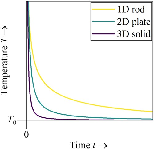
Table 1. Coefficients of the analytical cooling function; here, $a$ is the thermal diffusivity and is equal to $\lambda /c_{\mathrm{p}}\rho$. ${\alpha }_{\mathrm{c}}$, and ${\alpha }_{\mathrm{r}}$ are the heat transfer coefficients of convection and radiation, $U$ denotes the circumference, $A_{\mathrm{c}}$ represents the cross-sectional area of the 1D rod, and $h$ denotes the thickness of the 2D plate.

Case	Coefficient
	$c_{\mathrm{a}}$	$c_{\mathrm{b}}$	$c_{\mathrm{c}}$
1D rod	${\displaystyle \frac{Q}{A_{\mathrm{c}}{c}_{\mathrm{p}}\rho {(4\mathrm{\pi a})}^{0.5}}}$	${\displaystyle \frac{({\alpha }_{\mathrm{c}}+{\alpha }_{\mathrm{r}})U}{A_{\mathrm{c}}{c}_{\mathrm{p}}\rho }}$	$0.5$
2D plate	${\displaystyle \frac{Q}{h{c}_{\mathrm{p}}\rho (4\mathrm{\pi a})}}$	${\displaystyle \frac{2({\alpha }_{\mathrm{c}}+{\alpha }_{\mathrm{r}})}{h{c}_{\mathrm{p}}\rho }}$	$1$
3D solid	${\displaystyle \frac{2Q}{c_{\mathrm{p}}\rho {(4\mathrm{\pi a})}^{1.5}}}$	$0$	$1.5$

Model formulation

Equation (2), in conjunction with the expressions in Table 1, provides the analytical temperature histories for each of the three ideal cases. However, in the context of WAAM, the target geometries and their thermal fields during the manufacturing process are more complex. The thermal conduction conditions of a wall, for example, exhibit characteristics that resemble the 3D case during the initial layers and transition towards a behaviour that is closer to the 2D case at higher layers. Another consideration is that a wall is unevenly preheated from the welding of the previous layers and, therefore, favours or inhibits the heat conduction in particular directions. However, it is reasonable to anticipate that the temperature history will demonstrate similarities in geometries, where analytical solutions are not available, yet resemble the three ideal cases. Hence, the analytical solutions must be adjusted to better replicate the specific thermal behaviour of the WAAM process. Consequently, it is proposed to calibrate the constants $T_0$, $c_{\mathrm{a}}$, $c_{\mathrm{b}}$, and $c_{\mathrm{c}}$ within Equation (2) to adapt the cooling characteristics to non-ideal geometric elements, such as wall joints.

Depending on the number of walls connected to the joint, the local cooling conditions vary. A further distinction of the cooling function is made based on each vertex’s degree d, which is defined as the number of edges connected to the vertex. For example, the kite geometry in Figure 1 features one one-degree vertex (v₀), one two-degree vertex (v₄), and three three-degree vertices (v₁, v₂, v₃). A high-degree vertex signifies a part section with many walls connected to it, with each connection further increasing heat conduction. In contrast, a low-degree vertex has fewer connected walls, thus, impeding rapid heat conduction. Thus, the constants of the cooling function must be adjusted accordingly.

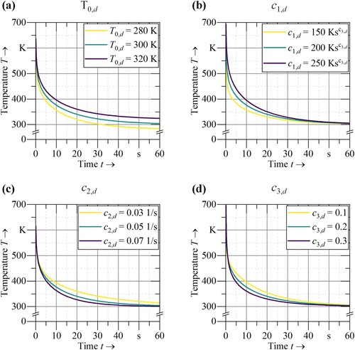
The cooling function of the SWS is given as (3) $T_{\mathrm{SWS},d}(t)=T_{0,d}+{\displaystyle \frac{c_{1,d}}{t^{c_{3,d}}}\exp (-c_{2,d}t),}$(3) where $T_{0,d}$, $c_{1,d}$, $c_{2,d}$, and $c_{3,d}$ are constants that characterise the cooling behaviour and are calibrated according to the vertex’s degree d. In Equation (3), each coefficient holds a distinct significance and can be interpreted as follows: The constant $c_{1.d}$ signifies an energy input, $c_{2,d}$ represents the rate at which the temperature approaches $T_{0,d}$, and $c_{3,d}$ denotes the rate of the temperature decrease near the initial point. The cooling function is exemplarily visualised in Figure 4 with sets of different values for the four constants.

Figure 4. Cooling functions (Equation (3)) using different exemplary values for (a) $T_{0,d}$, (b) $c_{1.d}$, (c) $c_{2,d}$, and (d) $c_{3,d}$.

Using the established thermal behaviour, the thermal simulation model for the SWS can be formulated. The time-dependent thermal history $T_i(t)$ at vertex ${\mathrm{v}}_i$ in the graph representation of a part is defined as (4) $T_i(t)=T_{0,d}+\sum _k(T_{\mathrm{SWS},d}(t-{\tau }_k)-T_{0,d}),$(4) where ${\tau }_k$ depicts the time at which the vertex ${\mathrm{v}}_i$ is reached by the welding torch for the $k$-th time and $d$ is the degree of the vertex ${\mathrm{v}}_i$. Thus, the temperature of a vertex is determined by a temporal superposition of cooling functions, depending on the number of times the node is traversed by the torch and the time passed between each traversal.

According to the model presented in Equations (3) and (4), the temperature value is infinite each time the welding torch passes a vertex ($t={\tau }_k$) due to the singularity in the fraction of Equation (3). In these cases, the temperatures were plotted at a slightly shifted time $\tilde{t}={\tau }_k+0.1\mathrm{s}$ instead. This choice did not impact the interpretation of the results significantly, as it corresponds to a relatively small timescale. However, it enhanced the visual clarity and the comprehension of the data.

Methodology

Calibration and validation procedures

The calibration and validation procedure for the SWS is shown in Figure 5 and followed a two-step workflow. The first step was the calibration and validation of the FE simulation using experimental data and the second step was the calibration and validation of the semi-analytical SWS model using the FE simulation results. The two-stage process was necessary due to the specific requirements of the SWS. The calibration of the SWS requires the temperature data directly on the surface of the welded layer, both shortly before and after the passing of the welding torch. This data is challenging to obtain reliably in experiments, as the arc would interfere with optical measuring equipment and the high temperatures in the process zone would destroy thermocouples. Moreover, as the top surface of a WAAM part is reapplied in each layer, a swift readjustment of the optical measuring equipment or a repositioning of thermocouples may be required in between layers. However, this temperature data can be easily retrieved from FE simulation results. Thus, the FE simulation was used as an intermediate step in the calibration and validation of the SWS. The validated SWS, in turn, enables the deposition sequence optimisation and its results are once again validated using FE simulation results.

Figure 5. Workflow of the calibration and validation procedures.

Experiments

Setup

Figure 6(a) illustrates the experimental setup inside the robotic welding chamber, and Figure 6(b) gives a detailed view on the specimen. The welding power source (TPS 400i, Fronius International GmbH, Austria) was installed on a 6-axis robotic arm (MH24 robot with a DX200 controller, Yaskawa Europe GmbH, Germany). The substrates used were AA 5083 (AlMg4.5Mn0.7) plates (Bikar Metalle GmbH, Germany), measuring 250 mm × 200 mm × 10 mm in width, height, and depth, and were fixed on a 2-axis welding and tilting table (DK250, Yaskawa Europe GmbH, Germany). The feed material was AA 5183 (AlMg4.5Mn0.7) wire with a diameter of 1.2 mm (Safra S.P.A, Italy) and the shielding gas was Argon 4.6 (Linde Gas, Germany). The chemical compositions of the materials are given in Table 2.

Figure 6. (a) Experimental setup inside the robotic welding chamber; (b) detailed view of the specimen; z is the build-direction.

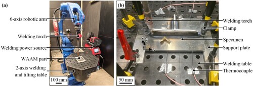
Table 2. Chemical compositions of the feed and substrate material according to the suppliers (ratios given in m.%).

	Element
	Si	Cu	Fe	Mn	Mg	Cr	Ti	Al
AA 5183 (wire)	0.04	<0.01	0.16	0.63	4.94	0.08	0.10	Balance
AA 5083 (substrate)	0.40	0.10	0.40	<1.00	4.90	<0.25	0.15	Balance

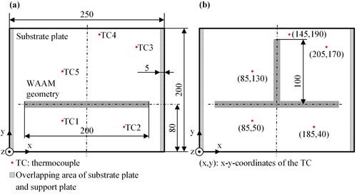
In order to calibrate and validate the FE simulation, two distinct WAAM geometries were produced: a straight wall and a T-joint. These geometries were selected due to their simplicity in the experimental execution and for providing one-, two-, and three-degree vertices required for determining the calibration constants. The substrate plate dimensions remained consistent across both geometries. A schematic representation of the two geometries used in the experiments is shown in Figure 7. Five boreholes with a depth of 5 mm and a diameter of 1.2 mm were drilled into the substrate plate to each fit a thermocouple (Type N, TC Mess-und Regeltechnik GmbH, Germany) for the temperature recording during the experiments. The positions of the boreholes remained the same for both specimen geometries and were selected to be at different distances to the WAAM geometry. The thermal data acquisition was conducted using a data logger (NI 9213 Module, National Instruments Corp, USA) with a sampling rate of 4 Hz. During the WAAM process, the substrate plates were placed on support plates along the shorter edges and were fastened to the table using clamps. This ensured uniform convection conditions across the whole surface of the specimen.

Figure 7. Schematic illustration of (a) the calibration wall geometry and (b) the validation T-joint geometry; all measurements and coordinates are given in mm; z is the build-direction

Manufacturing process

Two welding processes were used to manufacture the part. The Fronius cold metal transfer (CMT) Mix process was employed for the first layer of each specimen to ensure proper fusion between the WAAM part and the substrate material. The Fronius CMT Universal process was utilised to weld the remaining layers. The process speed was set to 10 mm/s while the wire feed speed was 6.5 m/min. A weaving pattern was implemented with a frequency of 2 Hz and an amplitude of 4 mm. This choice of welding parameters was based on a previous parameter study and resulted in walls with a thickness of 10 mm and an average layer height of 1.6 mm.

The calibration wall geometry, shown in Figure 7(a), measured 200 mm in length and comprised 20 layers. This arrangement yielded an average wall height of 32 mm. The layers were applied in a unidirectional manner. An interlayer dwell time was maintained between successive layers to prevent the part from overheating. The total interlayer dwell time was comprised of a predetermined waiting interval of 30 s, the traverse time from the welding end to the welding start position, and the preparation time of the welding power source before and after each welding process. This resulted in a total interlayer dwell time of 43.7 s.

In the T-joint validation geometry, shown in Figure 7(b), the short wall measured 100 mm in length and was orthogonally connected to the centre of the long wall measuring 200 mm in length. The deposition sequence of each layer involved applying the long wall first, followed by the short wall, which was welded from the free end towards the joint. Between the completion of the long wall and the welding start of the short wall, a 9.3 s dwell time was held. Moreover, an interlayer dwell time of 39.8 s was maintained before the start of the deposition of the next layer.

Finite element simulation

Setup

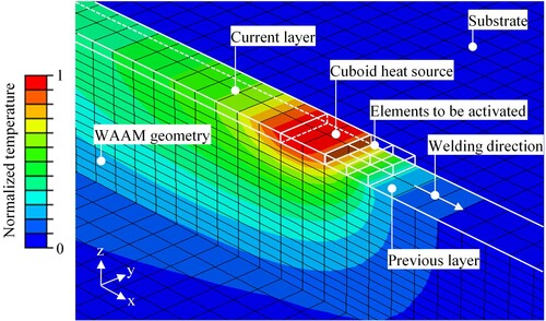
The software used for the transient thermal FEA was Abaqus FEA version 2020 (Dassault Systèmes SE, France). In the simulation, the heat input from the electric arc in the WAAM process was modeled using a cuboid heat source, while the material input from the melting of the wire was represented using local element activation (see Figure 8). At the beginning of the simulation, the elements of the WAAM part were deactivated. As the cuboid heat source followed a designated welding path, it activated elements along its trajectory until the whole part was printed. The welding trajectory was conveyed to the simulation software using a comma-separated value file, in which each line defined a temporal point, a spatial coordinate, and the corresponding power value of the welding torch. This approach facilitated the simulation of multi-layer components [18, 27]. The simulation result was the transient thermal field of the part during the WAAM process.

Figure 8. Simulation setup in the FEA software shown with an exemplary thermal fied; z is the build-direction

Material properties

For the used aluminum materials, the thermal material properties of the wire and the substrate were assumed to be equal due to the similar ratios of their main chemical components (see Table 2). The density $\rho$ was assumed constant at 2660 kg/m³, while the temperature-dependent specific heat capacity $c_p$ and the thermal conductivity $\lambda$ are given in Table 3. The material properties within the given temperature range were subjected to linear interpolation, while the maximum and minimum values were assumed to be constant at temperatures above or below the specified range.

Table 3. Temperature-dependent specific heat capacity and thermal conductivity [28] of AA 5083 and AA 5183 used in the FE simulation.

Temperature $T$ in $\mathrm{K}$	298	773
Specific heat capacity $c_{\mathrm{p}}$ in W/(kgK)	913.3	1,108.0
Thermal conductivity $\lambda$ in W/(mK)	121.5	169.0

Heat source and boundary conditions

Sophisticated heat sources, such as the Goldak heat source [29] are essential in welding or WAAM simulations that focus on the physical conditions at the process zone. However, when the simulation is directed towards the macroscopic thermal history of a WAAM part, such complexity becomes unnecessary [30–32]. The thermal simulations in this study target the macroscopic thermal history of WAAM parts, leading to the utilisation of a basic cuboid heat source adapted from [31,32].

The time- and space-dependent cuboid heat source $q(\mathit{x},t)$ is defined by: (5) $q(\mathit{x},t)=\eta {\displaystyle \frac{P(\mathit{x},t)}{\mathrm{hwl}},}$(5) where $\eta$ is the efficiency, $P(\mathit{x},t)$ is the power output of the welding power source at a particular position and time, and $h$, $w$, and $l$ denote the height, width, and length of the cuboid heat source, respectively. The convective energy dissipation $Q_{\mathrm{c}}$ at surfaces was considered using (6) $Q_{\mathrm{c}}=\mathrm{kA}(T_1-T_2),$(6) where $k$ represents the heat transfer coefficient between the part and the surrounding fluid, $A$ signifies the surface area on which the convection boundary is active, $T_1$ represents the temperature of the surface of the solid, and $T_2$ is the ambient temperature, which was set to 297 K in all simulations for this study. Due to the low emissivity of aluminum (${ϵ}_{\mathrm{Al}}\le 0.1$ [33]), the thermal radiation was excluded from the numerical model.

The calibration of the thermal FE model was achieved by iteratively adjusting the efficiency of the heat source $\eta$ and the convection coefficient $k$ until the simulated thermal history closely matched the measurements at the positions TC1–TC5 (see Figure 7(a) and Figure 7(b)). The power values of the heat source were taken from the log files of the welding power source. The thermal FE simulation was validated by comparing the simulation results to the measurements.

Mesh

A mesh convergence study was conducted to determine an appropriate element size for the thermal FE simulations in this paper. As the benchmark, the WAAM simulation of the wall geometry illustrated in Figure 7(a) was perfomed for a process time of 200 s, resulting in the simulated deposition of three layers. The number of linear hexahedral elements resolving the length, width, and height of each layer was systematically varied in three stages, with the element size in the WAAM geometry halfing between each stage. Figure 9 illustrates the three mesh configurations used in the mesh convergence analysis. The notation 50 × 2 × 1 signifies a mesh in which the length of a layer is resolved with 50 elements, the width with 2 elements, and the height with 1 element. The dimensions of the elements in the substrate plate were adjusted to the element sizes in the WAAM geometry. The temperature profiles at the selected points TC1, TC4, and C (see Figure 9(b)) were compared to the result of the finest mesh using the root mean squared error (RMSE). The points TC1 and TC4 refer to the respective thermocouple positions in Figure 7(a) and (b), while point C is an additional point introduced for this mesh convergence study and positioned at the centre on the first layer. The results of the mesh convergence study are given in Table 4.

Figure 9. Mesh configurations in the mesh convergence study, with (a) 50 × 2 × 1, (b) 100 × 4 × 2, and (c) 200 × 8 × 4 resolving the length × width × height of each layer; z is the build-direction.

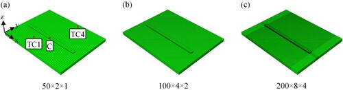
Table 4. Result of the mesh convergence study.

	Number of elements each layer (length × width × height)
	50 × 2 × 1	100 × 4 × 2	200 × 8 × 4
Number of nodes in -	15,273	100,405	435,125
Minimum element size (x × y × z) in mm	5.00 × 5.00 × 1.60	2.50 × 2.50 × 0.40	1.25 × 1.25 × 0.40
Computing time in s	125	673	3959
RMSE in K at TC1	0.09	0.03	0
RMSE in K at TC4	0.04	0.02	0
RMSE in K at C	0.85	0.61	0

Convergence is achieved even at the coarsest mesh (50 × 2 × 1), given the low RMSE values with a maximum of 0.85 K at point C. However, the computing time of the coarsest mesh consitutes 18.8% of the simulation time of the medium mesh (100 × 4 × 2) and only 3.3% of the simulation time of the densest mesh (200 × 8 × 4). Consequently, the coarsest mesh with the corresponding element size of 5.00 × 5.00 × 1.60 mm was selected for optimal performance in the simulations involving the wall geometry (see Figure 7(a)) and the T-joint (see Figure 7(b)). Simulations regarding the kite geometry (see Figure 1(a)) were executed with comparable element sizes, as identical welding parameters and boundary conditions applied.

Data processing for the simplified WAAM simulation

In the calibration process of the SWS, a particular data processing procedure is required for the thermal history results of the FE simulation. The data processing is exemplified by the centre three-degree vertex of the T-joint geometry with 50 layers in Figure 10.

Figure 10. Data processing of the thermal history; (a) mathematical graph and three-dimensional model of a T-joint geometry; z is the build-direction; (b) close-up of the central wall joint geometry and selection of considered cooling curve recording positions; (c) band of extracted cooling curves and their consolidated average plotted in the relative time scale $\theta$_.

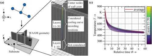
Each SWS vertex exists within a two-dimensional plane, yet it represents a wall joint geometry in the three-dimensional part in the FE simulation (see Figure 10(a)). In the FE simulation, the part is progressively constructed layer by layer. Thus, the heat source passes all wall joint locations at least once in every layer. With each heat source traversal, a wall joint undergoes a rapid heating and a following slower cooling process. The resulting thermal history recorded on the topmost layer at the wall joint location is a cooling curve, which is subsequently utilised for the calibration or validation of the SWS (see Figure 10(b)). Once all cooling curves were extracted from a wall joint location, the time-dependent temperature values were transformed into a relative timescale $\theta$, in which the time origin is shifted and aligns with the passing time of the heat source. An exemplary band of extracted thermal histories for a three-degree vertex is shown in Figure 10(c). The bands of temperature curves are then consolidated into a single average temperature curve. It is important to note that the cooling curves in the first ten layers were excluded from consideration due to their proximity to the substrate plate. This decision led to a decrease in the standard deviation during the calibration process, thereby enhancing the accuracy of the model.

The consolidated average thermal histories of each three-degree vertex were used to calibrate the four parameters, $T_{0,3}$, $c_{1,3}$, $c_{2,3}$, and $c_{3,3}$ in the cooling equation (refer to Equation (3)). The four parameters were determined by fitting the curve of the cooling equation to four equidistant points on the average thermal histories, ranging from the beginning to the end of the curve. The software used was MATLAB version 2022a (The MathWorks Inc., USA). The calibration process of one-, two-, four- and more-degree vertices is analogous.

In the validation process, the thermal history undergoes an identical data processing. However, the resulting average thermal histories from the FE simulation were not employed to determine calibration parameters. Instead, they served as reference to compare to and validate the SWS simulation results.

Deposition sequence optimisation setup

The optimisation aims to find the best deposition sequence of all possible deposition sequences for a given geometry in its mathematical graph form with respect to a certain optimisation criterion. A variation in deposition sequences between layers was not permitted. The optimisation procedure, together with the SWS, was implemented using Python 3.10.

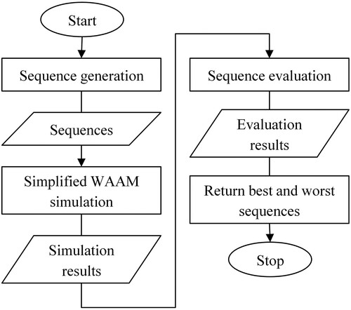
The workflow detailing this optimisation process is depicted in Figure 11. The workflow began with the creation of deposition sequences, in which all possible sequences were collectively generated using a full factorial design. The total number of possible sequences is a function of the number of edges in the mathematical graph form of the part. In the case of the kite geometry shown in Figure 2, which consists of six edges, the total number of possible deposition sequences was 6! · 2⁶ = 46,080 if welding in both directions along each edge was permitted. Subsequently, the sequences were simulated using the SWS. The sequence evaluation step began by identifying the maximum interpass temperature within each deposition sequence, which served as the score for that sequence. Subsequently, the lowest and highest scores across all deposition sequences were determined. The sequence with the lowest scores were considered the best, while the sequences with the highest scores were deemed the worst.

Figure 11. Workflow of the deposition sequence optimisation.

The deposition sequence evaluation can also be formulated as a mathematical optimisation problem. In reference to Figure 2(b), let $T_{\mathrm{int},i,k,s}$ denote the k-th interpass temperature at vertex ${\mathrm{v}}_i$ for the deposition sequence $s$, where $s$ = 1, 2, … , 46,080 represents each individual sequence. With the objective of minimising the maximum interpass temperature across all sequences, the best deposition sequences can be obtained by solving the optimisation problem: (7) $\underset{s}{min}\left(\underset{i,k}{max}{T}_{\mathrm{int},i,k,s}\right).$(7) Analogously, the worst sequences can be determined by solving the optimisation problem:

(8) $\underset{s}{max}\left(\underset{i,k}{max}{T}_{\mathrm{int},i,k,s}\right).$(8)

At the end of the deposition sequence optimisation, the best and the worst deposition sequences were returned.

The validation of the deposition sequence optimisation was conducted by comparing the interpass temperature distributions resulting from the best and the worst deposition sequences. To analyze the interpass temperature distribution, the transient thermal history field obtained from the FE simulation was extracted and transformed into a single time-independent interpass temperature field. The interpass temperature was continuously extracted from the nodes beneath the to-be-activated elements 2 s prior to the arrival of the heat source (refer to Figure 8). By performing this temperature extraction for every node within the part, an interpass temperature field was generated, allowing for a clear visualisation through a colour-coded scale.

Results and discussion

Calibration of the finite element simulation

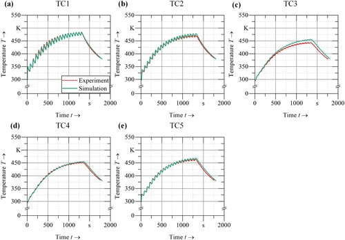
The resulting thermal histories from the calibrated FE simulation are presented in Figure 12 alongside the measured temperatures for all the considered positions. All temperature curves exhibited an oscillating pattern while increasing with process time. Each period represents the welding time and the subsequent dwell time of a layer. The thermocouples positioned closer to the wall (TC1, TC2) exhibited higher peaks and greater fluctuations during each period compared to those located farther away (TC3, TC4, TC5). This observation aligned with expectations, as thermal gradients were highest in proximity to the process zone and gradually diminished with increasing distance.

Figure 12. (a)–(e) Comparison between measurements and simulation results of the thermal histories of TC1–TC5 for the wall calibration geometry

For an efficiency $\eta$ of 0.88 and a convection coefficient $k$ of 17 W/mm², the R² values exceeded 0.99 and the maximum RMSE fell below 9 K for all measurement positions (see Table 5).

Table 5. R² values and RMSE of the calibrated model for all measurement positions TC1–TC5.

	Measurement position
	TC1	TC2	TC3	TC4	TC5
R^2 in -	0.9908	0.9946	0.9975	0.9962	0.9947
RMSE in K	4.00	5.08	8.71	3.13	3.89

Validation of the finite element simulation

The thermal measurements and the simulation results for the positions TC1–TC5 are shown in Figure 13. The R² values for the individual positions remained above 0.97 and the maximum RMSE increased slightly to 11.40 K (see Table 6). The simulation follows the measurements closely. The findings proved that the simulation model is a reliable tool in predicting the thermal history.

Figure 13. (a)–(e) Comparison between measurements and simulation results of the thermal histories of TC1–TC5 for the T-joint validation geometry

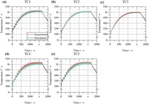
Table 6. R² values and RMSE of the validated model for all measurement positions.

	Measurement position
	TC1	TC2	TC3	TC4	TC5
R^2 in -	0.9724	0.9899	0.9961	0.9919	0.9883
RMSE in K	9.47	5.83	6.45	11.40	9.94

Calibration of the simplified WAAM simulation

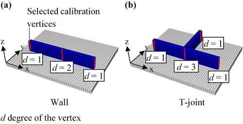
The calibration of the SWS was done using the validated FE simulation. For the SWS, the wall and the T-joint geometry were simulated with an increased number of 50 layers. Figure 14 illustrates the selection of vertices for the calibration of the parameters $T_{0,d}$, $c_{1,d}$, $c_{2,d}$, and $c_{3,d}$ of the cooling function.

Figure 14. Choice of calibration vertices for (a) the wall geometry and (b) the T-joint geometry for different vertex degrees d; z is the build-direction

The calibrated parameters, along with their corresponding R² and RMSE regarding the average FE result, are presented in Table 7 and plotted in Figure 15. The close correspondence between the simulated history and the analytical function demonstrates the ability of the cooling function to effectively approximate the cooling behaviour of various wall geometries with varying degrees of connections.

Figure 15. Cooling curves of the (a) one-, (b) two-, and (c) three-degree vertices using the calibrated parameters given in Table 7 and the cooling function defined in Equation (2).

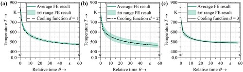
Table 7. Calibrated parameters for one-, two-, and three-degree vertices.

	Vertex degree
	$d=1$	$d=2$	$d=3$
$T_{0,d}$ in K	463.09	452.67	498.61
$c_{1,d}$ in Ks^c3	236.01	215.21	164.34
$c_{2,d}$ in 1/s	0.0388	0.0355	0.0876
$c_{3,d}$ in -	0.1922	0.1672	0.1787
R^2 in -	0.9951	0.9969	0.9991
RMSE in K	6.40	5.57	2.12

Validation of the simplified WAAM simulation

The validation of the SWS was performed using the kite geometry (see Figure 1), which comprised 50 layers. The kite geometry was first simulated using the validated FE simulation model. A deposition sequence was selected arbitrarily out of the 46,080 possibilities and is illustrated in Figure 16(a).

Figure 16. (a) Mathematical graph of an arbitrarily selected deposition sequence for the validation of the SWS; z is the build-direction; (b)–(f) comparison of FE and SWS results of the thermal histories at the vertices $v_0$–$v_4$.

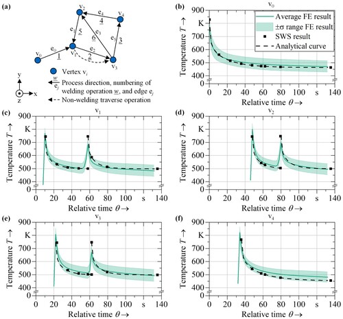
The Figure 16(b)–(f) show the comparison between the average thermal histories from the FE results at the vertices ${\mathrm{v}}_0$–${\mathrm{v}}_4$ in relation to the results from the calibrated cooling functions. As the vertices ${\mathrm{v}}_1$, ${\mathrm{v}}_2$, and ${\mathrm{v}}_3$ were traversed twice by the heat source in each layer, a second temperature peak in the respective temperature graphs occured.

The calibrated cooling functions followed the course of the average temperature histories well, as the corresponding semi-analytical temperature curves revealed a close match with the FE-simulated temperatures. The graphs show that, for the most part, the results obtained from the SWS fell within the $\pm \sigma$ range of the average thermal history computed by the FE simulation. This observation suggested a sufficient accuracy of the SWS. Simulation results exceeding the standard deviation threshold $\pm \sigma$ were mainly observed prior to the second temperature peaks for the thermal histories of ${\mathrm{v}}_1$, ${\mathrm{v}}_2$, and ${\mathrm{v}}_3$. This occurrence could be attributed to the FE simulation, where vertices located ahead of the heat source experienced preheating before its arrival due to heat conduction in the process direction. In contrast, the simplified model assumed an instantaneous arrival of the heat source, which accounts for these disparities. Table 8 shows the R² values and RMSE of the SWS model for the thermal histories at the vertices ${\mathrm{v}}_0$–${\mathrm{v}}_4$. The R² value surpassed 0.98 in the time intervals following the first temperature peak and remained above 0.97 for time intervals after the second temperature peak. The RMSE consistently remained below 28 K in all vertices.

Table 8. R² values and RMSE of the SWS model for the thermal histories at the vertices $v_0$–$v_4$.

	Vertex
	v0	v1	v2	v3	v4
R^2 in  – after the first peak	0.9899	0.9947	0.9954	0.9954	0.9877
R^2 in  – after the second peak	–	0.9893	0.9828	0.9770	–
RMSE in K after the first peak	13.58	12.38	22.77	24.26	27.09
RMSE in K after the second peak	–	17.71	14.95	12.18	–

Overall, the results demonstrated that the SWS was capable of effectively predicting the temperature histories within the selected vertices.

Validation of the deposition sequence optimisation

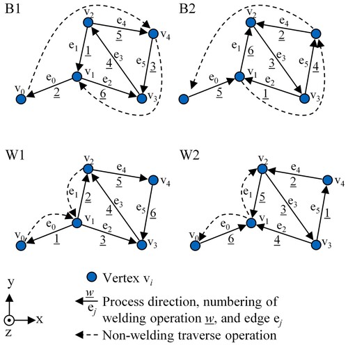
The deposition sequence optimisation with the objective of minimising the maximum interpass temperature was performed on the mathematical graph of the kite geometry shown in Figure 1(b). The optimisation setup yielded one palindromic pair of best and eight palindromic pairs of worst sequences. Figure 17 shows the mathematical graphs of the best pair of sequences (B1 and B2) and one of the worst pairs of sequences (W1 and W2) resulting from the optimisation.

Figure 17. Mathematical graphs of the investigated pair of the best (B1 and B2) and the worst (W1 and W2) deposition sequences; z is the build-direction.

In order to validate the optimisation results, the illustrated deposition sequences were simulated for 50 layers using the FE model, resulting in a total of four high-accuracy simulations. From the simulation results, the interpass temperature of each node of the WAAM part was extracted.

The difference in the interpass temperature is qualitatively depicted in Figure 18, in which elevated interpass temperatures are visible in the simulated parts utilising the worst deposition sequences compared to simulated parts using the best deposition sequences.

Figure 18. Visualisation of the interpass temperature of the investigated pairs of the best (B1 and B2) and the worst (W1 and W2) deposition sequences; z is the build-direction.

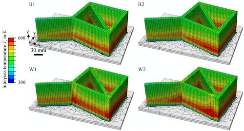
When the pair of best deposition sequences was compared to each other, no substantial difference was apparent. This observation remained consistent when considering the two worst sequences, where both sequences exhibit a concentration of elevated interpass temperatures near vertices v₁ and v₃. These findings also aligned with the optimisation results, as both the best and worst sequences were ranked equally by the optimisation in terms of the optimisation goal.

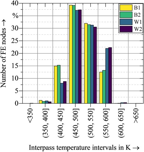
The conclusions were further substantiated by the histogram of the interpass temperature distributions shown in Figure 19. A significantly higher proportion of nodes from the worst sequences exhibited interpass temperatures within the range of 550 to 600 K, in contrast to the nodes from the best sequences. Conversely, notably more nodes from the best sequence experienced interpass temperatures in the range of 400 to 450 K compared to the nodes of the worst sequences. The quantity of nodes within each temperature range, however, remained consistent for the pair of the best as well as the pair of the worst deposition sequences.

Figure 19. Histogram of interpass temperature distributions for the best (B1 and B2) and the worst (W1 and W2) deposition sequences.

The results allowed the conclusion that the optimisation in combination with the SWS was able to find an optimised deposition sequence.

Computing time comparison

The FE simulations as well as the deposition sequence optimisations using the SWS were performed on the same workstation. The workstation was equipped with two AMD EPYC 75F3 CPU and 512 GB RAM. The computing times for both simulation approaches are given in Table 9. Each thermal simulation of the kite geometry (see Figure 1(a)) required 12,700 s or around 3.5 h on average, utilising multiprocessing with 8 CPU cores. In contrast, the computing time for all possible deposition sequences regarding the mathematical graphs of the kite geometry (see Figure 1(b)) amounted to 73.1 s when using one single CPU core. The computing time was further reduced to 25.5 s when also employing multiprocessing with 8 CPU cores. When both simulation approaches were compared to each other, conducting the simulation of one single sequence with the FE model demanded over 496 times the computational resources necessary for simulating all possible sequences with the SWS approach. This would translate to a projected duration of around 18.5 years for the FE model to compute all sequences.

Table 9. Comparison of computing times between the FE simulation and the SWS.

	Computing time for one sequence	Computing time for all sequences
FE (8 cores)	12,700 s	Projected: 18.5 a
SWS (8 cores)	< 0.001 s	25.5 s

The significantly faster computing time of the SWS model can be attributed to its semi-analytical nature, wherein only functions need to be evaluated in each time step. In contrast, the FE simulation requires solving large systems of equations, which is a much more time-consuming process. This also implies that the SWS can be executed on workstations with lower computational power compared to simulation servers often required for FE simulations. While the SWS outperform the FE simulation in terms of computing time, it is important to note that the SWS computes thermal histories solely at the few defined vertices of the part, while the FE simulation covers the entire domain in high resolution.

Conclusions and outlook

This study addressed the challenge of finding the optimal deposition sequence for thin-walled wire arc additive manufacturing (WAAM) parts amongst a vast amount of possible deposition sequences. A novel simplified WAAM simulation (SWS) was introduced, grounded on a semi-analytical cooling function derived from the analytical solutions to ideal geometries.

An experimentally calibrated and validated finite element (FE) model provided the calibration and validation data for the SWS. The validated SWS was then embedded into an optimisation. The key findings, in reference to the objectives of this paper, can be summarised as follows:

• It was possible to efficiently predict average thermal histories at specific locations within the part using the SWS. The calibrated cooling functions were able to follow the course of the average temperature histories from the validated FE simulation results within the $\pm \sigma$ threshold throughout most of the simulation time. Simultaneously, the SWS was significantly faster in terms of computing time than the simulation using the FE method.

• The deposition sequence optimisation with the embedded SWS was able to optimise the deposition sequence for the exemplary kite geometry (see Figure 1) regarding minimising the maximum interpass temperature.

However, following this successful proof of concept of the SWS, additional investigations and research should be conducted. The SWS is still held back by its limited applicability in scenarios involving changing process parameters, more complex geometries with both thin-walled and bulky parts, and other materials. The rapid simulation speed of the SWS came at the cost of an extensive calibration procedure involving specific experiments and FE simulations for each material and each parameter set. More efficient methods could be considered, in which the calibration parameters are derived or estimated from the equations given in Table 1 and known material data. Common materials utilised in WAAM, such as steel or titanium alloys, may be suitable candidates for further investigation. Furthermore, in the introduced optimisation process, all deposition sequences were generated and simulated, which is time-consuming. To improve the efficiency, more sophisticated optimisation algorithms, such as evolutionary algorithms or machine learning-based approaches, should be implemented. This approach is particularly recommended for larger, more complex parts with a higher number of edges and, thus, a higher range of deposition sequence possibilities. Moreover, the SWS should be extended to explore other optimisation criteria in future research. Instead of exclusively focusing on minimising the maximum interpass temperature, it could, for example, be applied for achieving an overall uniform temperature distribution throughout the entire WAAM part. This criterion and other criteria aimed at minimising stresses and distortions through the thermal field necessitate more intricate mathematical formulations and warrant further investigations. Lastly, adapting the SWS to other DED processes, such as laser metal deposition, is another future research direction that should be explored, given that DED processes operate under similar physical principles and encounter comparable challenges concerning deposition sequence selection.

Disclosure statement

No potential conflict of interest was reported by the author(s).

Data availability statement

The data that support the findings of this study are available from the corresponding author, Xiao Fan Zhao, upon reasonable request.

Additional information

Funding

This work was supported by the German Federal Ministry for Economic Affairs and Climate Action (BMWK) [grant number: 13IK002L].

References

- Wu B, Pan Z, Ding D, et al. A review of the wire arc additive manufacturing of metals: properties, defects and quality improvement. J Manuf Process. 2018;35:127–139. doi:10.1016/j.jmapro.2018.08.001
- Xia C, Pan Z, Polden J, et al. A review on wire arc additive manufacturing: monitoring, control and a framework of automated system. J Manuf Syst. 2020;57:31–45. doi:10.1016/j.jmsy.2020.08.008
- Cunningham CR, Flynn JM, Shokrani A, et al. Invited review article: strategies and processes for high quality wire arc additive manufacturing. Addit Manuf. 2018;22:672–686. doi:10.1016/j.addma.2018.06.020
- Williams SW, Martina F, Addison AC, et al. Wire + arc additive manufacturing. Mater Sci Technol. 2016;32:641–647. doi:10.1179/1743284715Y.0000000073
- Ma G, Zhao G, Li Z, et al. Optimization strategies for robotic additive and subtractive manufacturing of large and high thin-walled aluminum structures. Int J Adv Manuf Technol. 2019;101:1275–1292. doi:10.1007/s00170-018-3009-3
- Gu J, Bai J, Ding J, et al. Design and cracking susceptibility of additively manufactured Al-Cu-Mg alloys with tandem wires and pulsed arc. J Mater Process Technol. 2018;262:210–220. doi:10.1016/j.jmatprotec.2018.06.030
- Seow CE, Zhang J, Coules HE, et al. Effect of crack-like defects on the fracture behaviour of wire + arc additively manufactured nickel-base alloy 718. Addit Manuf. 2020;36:101578. doi:10.1016/j.addma.2020.101578
- Derekar K, Lawrence J, Melton G, et al. Influence of interpass temperature on wire arc additive manufacturing (WAAM) of aluminium alloy components. MATEC Web Conf. 2019;269:05001. doi:10.1051/matecconf/201926905001
- Ding D, Pan Z, Cuiuri D, et al. Wire-feed additive manufacturing of metal components: technologies, developments and future interests. Int J Adv Manuf Technol. 2015;81:465–481. doi:10.1007/s00170-015-7077-3
- Kozamernik N, Bračun D, Klobčar D. WAAM system with interpass temperature control and forced cooling for near-net-shape printing of small metal components. Int J Adv Manuf Technol. 2020;110:1955–1968. doi:10.1007/s00170-020-05958-8
- Zhao XF, Wimmer A, Zaeh MF. Experimental and simulative investigation of welding sequences on thermally induced distortions in wire arc additive manufacturing. RPJ. 2023;29:53–63. doi:10.1108/RPJ-07-2022-0244
- Venturini G, Montevecchi F, Scippa A, et al. Optimization of WAAM deposition patterns for T-crossing features. Proc CIRP. 2016;55:95–100. doi:10.1016/j.procir.2016.08.043
- Li F, Chen S, Shi J, et al. Thermoelectric cooling-aided bead geometry regulation in wire and Arc-based additive manufacturing of thin-walled structures. Appl Sci. 2018;8:207. doi:10.3390/app8020207
- Baier D, Wolf F, Weckenmann T, et al. Thermal process monitoring and control for a near-net-shape wire and arc additive manufacturing. Prod Eng Res Devel. 2022;16:811–822. doi:10.1007/s11740-022-01138-7
- Wu B, Pan Z, Ding D, et al. Effects of heat accumulation on microstructure and mechanical properties of Ti6Al4 V alloy deposited by wire arc additive manufacturing. Addit Manuf. 2018;23:151–160. doi:10.1016/j.addma.2018.08.004
- Li X, Lin J, Xia Z, et al. Influence of deposition patterns on distortion of H13 steel by wire-arc additive manufacturing. Metals (Basel). 2021;11:485. doi:10.3390/met11030485
- Israr R, Buhl JE, Elze L, et al. Simulation of different path strategies for wire-arc additive manufacturing with Lagrangian finite element methods. LS-DYNA forum, Bamberg, Germany. 2018.
- Zhao XF, Zapata A, Bernauer C, et al. Simulation of wire arc additive manufacturing in the reinforcement of a half-cylinder shell geometry. Materials (Basel). 2023;16; doi:10.3390/ma16134568
- Montevecchi F, Venturini G, Scippa A, et al. Finite element modelling of wire-arc-additive-manufacturing process. Proc CIRP. 2016;55:109–114. doi:10.1016/j.procir.2016.08.024
- Bähr M, Buhl J, Radow G, et al. Fügenschuh, stable honeycomb structures and temperature based trajectory optimization for wire-arc additive manufacturing. Optim Eng. 2021;22:913–974. doi:10.1007/s11081-020-09552-5
- Kadivar MH, Jafarpur K, Baradaran GH. Optimizing welding sequence with genetic algorithm. Comput Mech. 2000;26:514–519. doi:10.1007/s004660000195
- Viola R, Poulhaon F, Balandraud X, et al. Manufacturing time estimator based on kinematic and thermal considerations: application to WAAM process. Int J Adv Manuf Technol. 2024;131:689–699. doi:10.1007/s00170-023-11658-w
- Diestel R. Graph theory. Fifth edition Berlin, Heidelberg: Springer; 2017. doi:10.1007/978-3-662-53622-3
- Bondy JA, Murty USR. Graph theory with applications. New York (NY): North Holland; 1985, 1976. doi:10.1007/978-1-84628-970-5
- Zapata A, Benda A, Spreitler M, et al. A model-based approach to reduce kinematics-related overfill in robot-guided laser directed energy deposition. CIRP J Manuf Sci Technol. 2023;45:200–209. doi:10.1016/j.cirpj.2023.06.014
- Radaj D. Heat effects of welding: temperature field, residual stress, distortion. Berlin, Heidelberg: Springer Berlin Heidelberg; 1992. doi:10.1007/978-3-642-48640-1
- Zapata A, Zhao XF, Li S, et al. Three-dimensional annular heat source for the thermal simulation of coaxial laser metal deposition with wire. J Laser Appl. 2023;35:012020. doi:10.2351/7.0000813
- The European Union. Design of Aluminium Structures—Part 1–2: Structural Fire Design, Brussels, 2007.
- Goldak J, Chakravarti A, Bibby M. A new finite element model for welding heat sources. Metall Trans B. 1984;15:299–305. doi:10.1007/BF02667333
- Lindgren L-E. Computational welding mechanics: thermomechanical and microstructural simulations, first. Cambridge, Boca Raton: Woodhead Publishing; CRC Press; 2007.
- Ahmad SN, Manurung YHP, Mat MF, et al. Fem simulation procedure for distortion and residual stress analysis of wire arc additive manufacturing. IOP Conf Ser: Mater Sci Eng. 2020;834:012083. doi:10.1088/1757-899X/834/1/012083
- Ding D, Zhang S, Lu Q, et al. The well-distributed volumetric heat source model for numerical simulation of wire arc additive manufacturing process. Mater Today Commun. 2021;27:102430. doi:10.1016/j.mtcomm.2021.102430
- Touloukian YS, Dewitt DP, Touloukian YS (Eds.). Thermophysical properties of matter: The TPRC data series; a comprehensive compilation of data. New York (NY): IFI/Plenum; 1970.