Adjuvant therapies of bone graft around non-cemented experimental orthopedic implants stereological methods and experiments in dogs

List of papers

The PhD thesis is based on the following papers:

1. The effect of pretreating morselized allograft bone with rhBMP‐2 and/or pamidronate on the fixation of porous Ti and HA‐coated implants Baas J, Elmengaard B, Jensen TB, Jakobsen T, Andersen NT, Soballe K.

   Biomaterials. 2008 Jul;29(19):2915–22.

2. The bovine bone protein lyophillisate Colloss improves fixation of allografted implants ‐ a study in dogs

   Baas J, Lamberg A, Jensen TB, Elmengaard B,

   Soballe K.

   Acta Orthop. 2006 Oct; 77(5): 791–8.

3. Ceramic bone graft substitute with equine bone protein extract is comparable to allograft in terms of implant fixation ‐ a study in dogs Baas J, Elmengaard B, Bechtold J, Chen X, Soballe K

   Accepted by Acta Orthopaedica

The papers will be referred in the text by their Roman numerals (I‐III)

Institutions

Faculty of Health Sciences,

University of Aarhus, Denmark

Orthopaedic Research Laboratory

Department of Orthopedics Aarhus University Hospital, Denmark

Interdisciplinary Nanoscience Center (iNANO),

Department of Physics and Astronomy,

University of Aarhus, Denmark

Main supervisor

Prof. Kjeld Søballe, MD, DMSc

Department of Orthopaedic Surgery,

Aarhus University Hospital, Denmark

Project supervisors

Brian Elmengaard, MD, PhD

Department of Orthopaedic Surgery,

Aarhus University Hospital, Denmark

Thomas Bo Jensen, MD, PhD

Department of Plastic Surgery,

Arhus University Hospital, Denmark

Preface

This thesis is based on experimental studies performed at the Orthopaedic Research Laboratory, Department of Orthopaedics, Aarhus University Hospital, during my enrolment as a PhD student at the Faculty of Health Sciences, Aarhus University, 2004–2007.

My employment as a research fellow was financed by the Aarhus University Hospital and the Interdisciplinary Nanoscience Center (iNANO) at Aarhus University.

The experimental surgeries were done in part at the Clinical Institute, Aarhus University (studies I and II), and at the Animal Care Facilities, Hennepin County Medical Centre, Minneapolis, USA (study III). Preparation and sectioning of tissue and following evaluation was done at Orthopaedic Research Laboratory, Aarhus University Hospital.

I thank my supervisors for their invaluable advice and hard work, and especially my main supervisor Kjeld Søballe for providing excellent conditions for research throughout the studies. The Orthopaedic Research Laboratory at Aarhus University Hospital has been a fantastic scientific workspace in all respects, and I thank my colleagues and coauthors for this, in particular Thomas Jakobsen. These studies could not have been done without the knowledge and skills of lab technicians Jane Pauli and Anette Milton. I thank Joan Bechtold and my friends in Minneapolis for our good cooperation. I also wish to thank my father, Nils Baas, for mathematical and methodological counselling throughout the course of this work, Hans Jørgen Gundersen for stereological advice and Niels Trolle Andersen for statistical help. Finally, I thank my wife Christina and daughter Ella Marie for helping me maintain focus on what really matters, and for making it all worth while.

Acknowledgements ‐ Disclosures

The studies were financially supported by the following non‐commercial institutions:

• Augustinusfonden

• Beckettfonden

• Brødrene Hartmanns Fond

• Danish National Research Foundation, Grant No. 2052‐01‐0049 Interdisciplinary Nano‐science Center (iNANO)

• Danish Orthopaedic Society; DOS‐fonden

• Frimodt‐Heineke Fonden

• Göran Bauer Grant

• Korningfonden

• NIH, Grant No AR4205

The studies have benefited from institutional research support received from the commercial companies Danfoss AS and Ossacur AG, both of which have ownership interests in the medical devices Colloss, Colloss E and Ossaplast.

The following companies contributed with materials:

• Biomet Inc.: Implants

• Ossacur AG: Colloss, Colloss E and Ossaplast

• MaynePharma: Pamidronate

During the course of the PhD study, I have been involved in research that has benefited from institutional research support from the following companies with commercial interests in this research area:

• DePuy

• Zimmer

• Biomet

• Ortotech and Wright Medical

• Medtronic

• Novartis

Abstract

Revision arthroplasty is a challenging aspect of the otherwise quite successful area of joint replacement surgery. The instable interaction between implant and host bone has often initiated a destructive process of inflammation and osteolysis, rendering the revision site sclerotic and with insufficient bone stock. One way of dealing with this is to build up a bed of tightly packed morselized bone graft to support the revision implant in a procedure often referred to as impaction grafting. Fresh frozen morselized femoral head allograft is the gold standard material for impaction grafting of the large defects usually involved in revision arthroplasty. The clinical outcome does not match that of primary arthroplasties. Implant subsidence is greater, implant survival shorter, and the bone graft is often not incorporated into living bone.

The studies constituting this thesis have investigated ways of improving early implant fixation and bone graft incorporation. All studies used the same experimental canine model of early fixation and osseointegration of uncemented implant components inserted into a bed of impacted bone graft.

Study I compared bone grafted implants where the morselized allograft was used alone or had been added rhBMP‐2, the bisphosphonate pamidronate or a combination of the two. The main object was to see wether the previously observed growth factor related accelerated allograft resorption could be counteracted by the addition of an anti‐catabolic drug. The study also compared HA‐coated and non‐coated porous Ti implants. The untreated control implants had better mechanical fixation than all other treatment groups. RhBMP‐2 raised the total metabolic turnover of bone within the allograft with a net negative result on implant fixation. Pamidronate virtually blocked bone metabolism, also when combined with rhBMP‐2. The HA‐coated implants had more than twice as good mechanical fixation and improved osseointegration compared to the corresponding Ti implants.

Study II investigated the addition of a bovine bone matrix lyophilisate (Colloss^®) to the allograft in three different doses. The main object was to see, whether the addition of a biological delivery device of low‐dose osteogenic growth factors could provide a sufficient signal to increase the bioactivity of the bone graft without also yielding mechanical instability through increased allograft resorption. Allograft resorption increased with increased signal dose, but not to the extent that it affected implant fixation negatively at the observational time point. Mechanical implant fixation was doubled, and implant osseointegration and graft incorporation were improved.

Study III compared a β‐TCP ceramic bone graft substitute (Ossaplast^®) with and without an osteogenic signal (Colloss^® E) to morselized allograft with and without the same signal. The object was to investigate, whether the addition of an osteogenic stimulus to a bio ceramic could replace biological allograft bone. The addition of an osteogenic signal improved early osseointegration of implants grafted with β‐TCP granules and increased their mechanical implant fixation to a level comparable to the allografted implants.

All studies I‐III confirmed that the topical addition of an osteogenic signal could increase implant osseointegration and the formation of new bone within a grafted defect. Another striking observation was the near‐complete absence of fibrous tissue in the treated groups. The osseointegration of ceramic bone grafts improves when both the osteoconductive as well as the osteogenic components of bone are substituted. The effect on implant fixation of devices and pharmaceuticals that influence bone metabolism can be difficult to predict, as shown in study I. There seems to be a therapeutic window for these substances. This must be further explored prior to clinical use, as the adverse effects of overdosing bone anabolic and anti‐catabolic substances can be detrimental

Background

The success of most joint replacements is measured in ten‐year implant survival rates with revision as endpoint. According to the Danish Hip Arthroplasty Registry (1), the ten‐year survival rate for patients over 75 years is 95%, but only 86% in patients under 50 years age. Of the 8762 THRs performed in Denmark in 2006, 12.7% were revisions. The tendency towards younger and more active patients means that an average joint replacement undergoes increasing mechanical demands over an increasing number of years combined with often higher expectations to functionality. An increasing number of patients are therefore expected to need one or more revisions of failed implants during their lifetime.

Failure of implants has serious consequences for the patient. The loosening process is painful and debilitating, and the functional outcome of a revision is poor compared to the primary arthroplasty. The implant survival rate is lower and decreases with the number of re‐revisions. Young patients receiving joint replacement surgery are facing a considerable risk of serious physical disability and inability to work within a twenty‐year time frame (94).

Bone loss is one of the most challenging problems in revision surgery. The revision of a failed implant often involves severe periprosthetic osteolysis caused by mechanical instability, wear debris and/or infection. Further bone is often lost during the actual revision, and the bone anchoring the implant is often osteoporotic because of stress shielding. At revision, insufficient bone stock can be dealt with by using custom‐designed implants, metal augments or change of implant fixation site such as with long‐stemmed components in the hip. These solutions do not directly address the problem of the bone loss, and the problem might be even worse at later re‐revisions.

One way of managing bone loss is the use of bone grafts. Bone grafts can be used in osteolytic lesions to secure direct fit of the implant to bone in cementless reconstructions. Impaction bone grafting has become a common procedure to completely replace insufficient bone stock and secure mechanical support of the implant. Furthermore, it is thought that the bone graft scaffolds new bone formation and is replaced by the patient's own bone over time, providing a good bone stock for fixation of future revision implants. However, studies have shown that this is not always the case with impacted bone graft: It is often not completely resorbed, but remains encapsulated in fibrous tissue within the host bone many years after the transplantation (59;96;100)

Biological treatments to augment bone healing are increasingly being used in clinical orthopaedic practice. Osteogenic growth factors within the TGF‐ ‐superfamily induce anabolic responses in bone repair. These growth factors are embedded within the matrix of biological bone, and constitute the workhorse of the osteoinductive properties of demineralized bone matrix (DBM). Human BMP‐2 and BMP‐7 have been engineered by recombinant techniques and are already used clinically for fracture repair and spinal fusion. Bisphosphonates are anti‐catabolic drugs used primarily in the treatment of osteoporosis, but have also been used experimentally for reducing bone resorption around implants and in traumatized bone.

There is yet little information on the effects of these biological treatments on bone grafts used in implant fixation, and the information available is partly discouraging. Experimental as well as clinical data suggests that certain osteogenic growth factors can indeed promote implant osseointegration and new bone ingrowth, but also accelerate bone resorption, rendering especially allografted implants mechanically unstable (43;53).

Early bone grafting

In 1668, the Dutch surgeon Job van Meekeren repaired a traumatic defect in a soldier's cranium with a bone graft taken from the skull of a dog. The operation was clinically successful, but led to the patient's excommunication (14;64). It took another 250 years before bone grafting procedures became relatively common, much attributed to Fred Houlette Albee's bone grafting techniques published in 1915 (4). Albee also described the use of calcium phosphates as a replacement for biological bone grafts. Marshall Urist identified “bone formation by autoinduction” in 1965 (99), and the biological control mechanisms for bone formation were unveiled with the discovery of the first bone morphogenetic proteins responsible for this phenomenon (105).

A precursor to impaction bone grafting was the use of autograft bone chips and cement in the treatment of bone stock deficiency in protrusio acetabuli secondary to rheumatoid arthritis in the early seventies (33). Experimental evidence for the biological incorporation of cemented autologous bone grafts in acetabular wall reconstruction was provided in 1983 (77), and verified as clinically successful in 1984 (65).

Bone grafting in reconstructive joint surgery

In 1984, Slooff introduced a modified technique described as impaction bone grafting of the acetabular component. The technique involved defect containment with a metal fibre mesh, tightly packed allograft bone chips and pressurized cement between graft and implant. The first attempts on supporting femoral stems abandoned the principle of bridging or filling the areas of bone loss with long and bulky revision implants. Instead, the circumferentially restrained proximal femoral envelope was packed with morselized cancellous allograft, thus constructing a neomedullary canal. Initial uncemented techniques lead to many cases of subsidence, but this was prevented by the use of cement, where polymethylmethacrylate inserted under pressure provided the initial stability for the stem‐cement‐graft construct.

Impaction bone grafting is currently used for managing deficient bone stock with and without cement, and there is no sharp definition of when cement should be applied. Both techniques aim at restoring insufficient bone stock by replacement of the allograft with the patient's own bone over time (67;83). The cemented technique considers the often smoothened or defective wall of the revision cavity and allows pressurized cement to interdigitate between the allograft chips and the implant for increased fixation stability. The uncemented technique considers the benefit of direct bone to implant contact and applies impacted allograft as filler for contained defects. A study comparing impaction bone grafting of femoral revisions reported no difference in outcome between the two techniques (73). However, the study was not randomized and the choice of technique was based on the perioperative evaluation of the revision cavity.

Impaction grafting in revision total hip replacement has produced good medium‐ to long‐term results on both the acetabular and the femoral side. On the acetabular side, the overall survival rate with aseptic loosening as the end point, was 94% at 11.8 years (84;86). On the femoral side, the early series of Gie (25) and Elting (20) reported low short term rerevison‐ and complication rates. Later series have reported early subsidence of over 10 mm in 10% of the patients and subsidence of over 5 mm in another 10%, which were also associated with thigh pain (19). Meding et al (63) followed 34 patients over a mean of 30 months with good clinical results as measured by an increased average Harris hip score from 51 to 87 and low pain, but also thirteen cases of early subsidence and six intraoperative fractures. Comparable high rates of intraoperative complications were also reported in a retrospective study comparing cemented and uncemented techniques (73), but Lind et al.'s prospective series of 87 revisions in 80 patients over 3.6 years reported a promising combination high patient satisfaction, an increase in Harris hip score from 51 to 87, and a very low incidence of complications, subsidence and re‐revisions (57).

It is difficult to document to which extent impaction grafting contributes positively to revision implant survival. The outcome following revision arthroplasty has always been substantially worse than that after primary arthroplasty, and after subsequent revisions even worse. In Denmark, the 10‐year survival for the first revision of a THR is 80% and for the second revision it is 70% (1). From many of the reported series of bone‐grafted revisions, it may seem that this technique could be advantageous in terms of implant survival rate. However, their comparability is limited by study design, and clinical scores that are not validated for revised joint implants and also do not necessarily reflect improvements in long‐term implant survival. The survival stratified by revision methodology is not well described. Similarly, the contention that impaction increases survival of later re‐revisions remains poorly documented but is widely accepted based on experimental and retrieval studies, indicating that bone grafting regenerates the bone stock (83).

Early implant migration → late loosening

The importance of early implant osseointegration was introduced in the early eighties with the finding that dental implants tended to either fail within the first year after implantation or remain functional throughout the patient's life (2). Using roentgen stereophotogrammetric analysis (RSA), Kärrholm and colleagues (51) found that a migration of 0.33 mm of a cemented femoral hip arthroplasty component during the first postoperative 6 months was highly predictive of clinical failure leading to revision surgery within 5 to 8 years. The same tendency was confirmed the same year for uncemented femoral stem components by plain radiographic images (52) and later for uncemented knee components by RSA (80). This early indicator of a late event has shortened the observation time and allowed evaluation in randomized trials prior to clinical introduction of new implant technologies. Analogous to this, one of the key experimental research areas has been to promote early implant fixation.

Goals for early experimental implant fixation

Since good mechanical fixation at an early time point is important, it is of interest to know which biological parameters influence the magnitude of the mechanical fixation and in which way. No analysis of the relationship between mechanical fixation and periimplanteric biology has been published. An analysis of six clinically well‐functioning HA‐coated acetabular cups retrieved at autopsy 3.3 to 6.6 years after implantation had a mean percentage of bone‐implant contact of 36.5% (95). In lack of better reference, this compares to the typical fibrous tissue encapsulation of implants retrieved at revision. Experimentally, mechanical fixation also seems to be related to new bone formation and bone ongrowth, and inversely related to fibrous tissue formation (56;87).

The importance of direct bone‐to‐implant contact is more controversial for implants surrounded by bone graft. Retrieval studies have shown that clinically well‐functioning impaction‐grafted revision implants are often surrounded by a more or less inert composite of necrotic allograft bone chips and fibrous tissue (59). On an experimental basis, it has been suggested that this can even be advantageous in a process called fibrous tissue armouring, and that complete osseous remodelling may not be necessary to obtain a good clinical result with a morselized impacted graft (92). However, these studies lack a reference group in which the implant and bone graft is well osseointegrated, and therefore do not contribute decisively to which biological parameters are important for implant fixation.

It is therefore widely accepted, that also uncemented implants surrounded by bone graft should be well osseointegrated and that the patient's own bone should infiltrate the bone graft and replace it over time.

Based on this, the main goal of the experimental work of this thesis has been to improve early mechanical implant fixation. The results have been supplemented by histomorphometry, by which the tissues surrounding the implant have been quantified. This information was meant to substantiate any observed changes in mechanical implant fixation with different interventions in treatment, and, if possible, to provide a biological explanation for them. The assumptions were that improved implant fixation was associated with improved osseointegration, increased new bone formation, controlled resorption of the bone graft material and reduced fibrous tissue formation.

Animal models of impaction bone grafting

Whereas mechanical implant fixation can be evaluated by RSA, there is no equivalently good non‐invasive way of evaluating the tissues or metabolic processes surrounding an implant. Much of the understanding of this is therefore derived from experimental models of implant fixation. This is also the case for understanding the biology of impaction bone grafting.

The experimental models using functional implants are highly representative of the clinical situation. They have been used in several descriptive studies of periimplant biology, but may not be the best for evaluating different treatments. Schimmel and colleagues studied impacted grafts in goat acetabuli and found complete bone incorporation with bone remodelling into vital lamellar bone within 24 weeks. After longer observation periods, interface formation and aseptic loosening of the cups were seen (82).

Schreurs et al evaluated a primary THR where the femoral stem was cemented into a bed of impacted morselized allograft bone in goats (83). The scarce metaphyseal trabecular bone and the hard and smooth endosteal surface of goats was found to be a good model for the sclerotic endosteum encountered in revisions. Initial in vitro mechanical work on the model showed that the initial mechanical stability of the stems was good (85). The model showed that cement penetration into the graft material was at least 1 mm, but often penetrated the entire graft bed and reached the cortical wall. Graft incorporation and bone apposition was preceded by infiltration of loose connective tissue and vascular elements from the endosteal cortex progressing inwards. The histological picture at healing seemed to be trabeculae of new bone with incorporated graft chips stretching from the endosteal cortical surface towards the cement, with higher bone density near the cement mantle, but with fibrous tissue interposing between bone and cement. Graft that was surrounded by cement was not incorporated into vital bone. Incorporation and vascularization was present at 6 weeks, but not fully completed even after 12 weeks.

The trade‐off to the model's high clinical resemblance may be lower variable control. Two out of twelve implants were infected and one loose at 12 weeks observation time. The RSA data were not always consistent, as was the progression of healing between animals. Even in a paired design, this could cause difficulties in comparative intervention studies on this model.

The bone conduction chamber consists of a cylindrical interior space of 2 mm diameter and 7 mm height (103). One of the cylindrical ends is screwed into epiphyseal bone, from which cells are recruited into the chamber interior and tissues formed. The bone ingrowth distance into the chamber is determined by histology. The model has been used to describe bone grafts with different degrees of compaction (91) and under the influence of growth factors and bisphosphonates (48). Whereas the model has a good variable control, it has no implant from which data on fixation strength and degrees of osseointegration can be extracted. Another limitation is the location outside of load‐transmitting bone, which means that the wave of bone formation up through the chamber is often followed by subsequent resorption.

Morselized allograft bone

Allograft bone is considered a mechanically stable, osteoconductive scaffold for new bone formation. Furthermore, it is widely believed to contain some osteoinductive capacity (104), as it may stimulate new bone formation through its own resorption by the coupling effect. Shortly after impaction it recoils (97), adding initial stability to the implant. When host tissue invades the grafted space, the biomechanical properties of the composite changes. Incorporation of impacted allograft bone is fastest during the first six months (59) and radiographic examinations show little change after two years (20). Positron emission tomography (PET) has been used to evaluate the metabolic events around the femoral component of a hip implant after impaction grafting. Already after eight days there was activity corresponding to neovascularization and mineralization, but this was diminished after one year (90). Even fibrous tissue ingrowth alone appears to increase strength, and it has been suggested that this is sufficient for implant fixation (92). Cadaver studies have confirmed that fibrous tissue encapsulation of the graft chips is often the case (59;98); however, it is widely accepted that the grafted implant ideally should be osseointegrated, and the bone graft incorporated into, and with time replaced by, the patient's own bone.

Fresh frozen morselized allograft is considered the gold standard for grafting large defects around implants (94). The amount of autograft bone that can be harvested is limited and associated with donor site pain and morbidity (28). Allograft bone is, however, also only available in limited supply and of inconsistent quality (49).

Allograft bone for bone grafting procedures is supplied by tissue banks or dedicated bone banks. It is donated post‐mortem or by living patients, a typical example being the femoral head at hip replacements on fracture indication. It must be presumed, however, that the average donor has a higher age and a higher incidence of osteoporosis than a representative cross section of the population. It therefore seems fair to assume, that the quality of allograft bone has a high variability at best (72).

Allograft bone may transmit disease (10). Modern allografting using material stored within regulated bone banks has largely overcome this problem, and it is very rare when comparing the reports of infection versus the number of allografts distributed per year in the US (49). Allograft bone is to some extent processed by washing or gamma radiation to prevent disease transmission, but this may impair the mechanical and biological properties of the allograft (13). Tissue transplantation safety largely relies on infectious disease screening of donor and cultures from the transplant (49). Allograft bone can also provoke a substantial immunological host response, which is thought to compromise osseointegration and new bone formation. Some studies have indicated that donor‐recipient human leukocyte antigen (HLA) mismatch may result in poor graft incorporation despite a low cellular density (26;27), but allografts are generally not tested for histocompatibility.

Bone graft substitutes

Because of the risks, inconsistent quality and limited availability of biological bone grafts, it has long been of interest to find viable replacements for allograft bone. Whereas bone consists of both organic and inorganic components, most commercially available ceramic bone substitutes are pure inorganic materials such as hydroxyapatite and tricalcium phosphate. These materials provide an osteoconductive scaffold on which new bone can be formed and incorporated (55). Some are labelled bioactive, indicating cell‐mediated mineralization intimately related to bone matrix directly on the surface of the material.

The vast majority of bone graft substitutes are ceramic calcium phosphates, such as tricalcium phosphate and hydroxyapatite or biphasic combinations of these. Calcium phosphate cements are also marketed along with composites of calcium phosphates and collagen matrix proteins (12;91). Calcium phosphate ceramics are produced in different sintering processes. Theoretically, they can be designed as biphasic compounds and even composites to meet specific requirements in crystallinity, stoichiometry, porosity, interconnectivity, size, and shape. These material properties largely determine clinically important parameters such as strength, toughness, resorption rate and osseointegrative ability. Much research is currently being done on defining the ranges of the material properties that give the best outcome with regard to the clinical parameters. This is challenging, since many of the material parameters are inversely related and therefore highly dependent on the intended clinical application. Some rough guidelines do exist in terms of inciting osseointegration, such as a level of total porosity of at least 50–60%, a minimal diameter of interconnecting channels of 50–100 μm, and a level of strut porosity of at least 20% (35).

The advantage of ceramic bone graft substitutes is the prospect of application‐directed custom design of the material, highly controlled material properties with low variability, relatively low production costs, and simple shelf storage. These is, as of yet, more an expectation of an ongoing technological development than a current reality. So far they are reported as promising bone graft extenders rather than actual bone graft substitutes (44;101). This is partly due to mechanical limitations of ceramics, such as low viscoelasticity and high brittleness, and partly because ceramics contain no osteogenic signal, and do not exhibit the same level of bioactivity as allograft bone (15).

Bisphosphonates

Bisphosphonates is an anti‐catabolic class of drugs. They are synthetic organic analogues of pyrophosphates and have an equivalently strong affinity to hydroxyapatite. This bond is so strong that it for practical purposes can be considered permanent until the bone is resorbed. The biological effects of bisphosphonates were discovered around 1968 by Fleisch et al (23). They inhibit bone resorption by inducing osteoclastic inactivation or apoptosis.

The cellular mechanisms causing the effect of bisphosphonates have only recently been understood. First‐generation bisphosphonates are metabolized into cytotoxic ATP analogues (78). The more potent N‐bisphosphonates inhibit FPP synthase, an enzyme of the mevalonate pathway, by which protein prenylation is inhibited (61) rendering membrane proteins unable to incorporate into the cell wall (21). The bisphosphonate used in study I, pamidronate, is an N‐bisphosphonate.

Whereas the inhibitory effect on osteoclastic bone resorption is well established, recent evidence also suggests that bisphosphonates can initiate osteoblastic differentiation (75) and upregulate BMP‐2 gene expression (22;37;102). These effects are under investigation and the evidence still scarce and contradictory (39).

Since both first‐ and second‐generation bisphosphonates act by interfering with ubiquitous metabolic processes and pathways, it seems highly unlikely that bisphophonates should be able to act on osteoclasts only. The effect on osteoclasts in particular is therefore most likely due to a common accumulation on exposed mineralized surfaces. There may be some selectivity with regard to which cells can be influenced, as most bisphosphonates' ability to penetrate the cell wall without an active process such as pinocytosis is very limited due to the bulkiness and negative charge of the phosphonate group (66;79). One cellular requirement for cell death due to bisphosphonates may therefore be the capacity of endocytosis‐like membrane transport.

When a bisphosphonate is administered systemically, most of the drug that is not excreted renally will accumulate at sites of active bone metabolism (81) and bind to hydroxyapatite. Bound to the skeleton, it becomes metabolically inactive (76). It is released from this inactive state in the body when the bone is resorbed through remodelling or other bone‐metabolic events. In its unbound state it is again available for either rebinding to hydroxyapatite or cellular uptake by endocytosis. Since the osteoclasts are highly endocytic during the bone resorption process that caused the release of the bisphosphonate, it is likely to be internalized in the very osteoclasts causing its release from the skeleton. The accumulation of bisphosphonate in the osteoclast leads to its reduced activity or death, by which the local bone resorption is reduced.

It is noticeable that bisphosphonates bind to sites in the skeleton with metabolic activity at the time when the compounds were systemically available, and that bisphosphonates exert their anti‐catabolic effect locally by inhibiting the very osteoclasts that have facilitated their release from bone. This means that bisphosponates inhibit their own release and metabolism and are, to some extent, self‐preserving. This can be beneficial for the treatment of chronic conditions like osteoporosis, but has also given rise to concerns about a decreased ability to clear bacterial infections in the bisphosphonate‐treated skeleton. Bisphosphonates have also been the subject of interest as well as concern in treating, maintaining or potentially accelerating bone pathologies involving osteonecrosis. One strategy could be to preserve dead or dying bone for mechanical support and scaffolding new bone formation, another to clear the pathology and stimulate the formation of vital bone (5). Finally, there have been concerns about disrupting the coupled balance between bone resorption and bone formation by the use of bisphosphonates, but this seems to be of lesser importance in traumatic bone healing than in normal bone turnover (60).

These considerations are closely related to the thought of using bisphosphonates in combination with allograft bone: preservation of the mechanically stable allograft pending remodelling of the newly formed, still mechanically weak woven bone into strong lamellar bone. This was found relevant for the early catabolic events of any grafted defect (90), but in particular in the combination with a bone anabolic adjuvant therapy known to accelerate not only new bone formation but also bone resorption (89).

The systemic administration of a bisphosphonate requires exposed mineralized bone and vascularization. Vascularization in the grafted defect occurs early, but not immediately, and progresses from the vital perimetry of the defect towards the implant or cement mantle. Combined with the low bioavailability of bisphosphonates, the timing of the relatively high doses needed could be complicated. Bisphosphonates have been successfully administered systemically in experiments with allograft (7;42), but most studies have evaluated topical administration showing a consistent ability to preserve bone or allograft bone, but inconsistencies in terms of maintaining the host bone's ability to form new bone and maintain implant stability (6;40;41;48;54;88).

Bone growth factors

Isoforms of transforming growth factor beta (TGF‐) and bone morphogenetic protein (BMP) stimulate the recruitment, proliferation and differentiation of osteoblastic progenitor cells, and are potent local anabolic agents in bone repair. BMPs are embedded within the bone matrix in minute amounts; approx. 1–2 μg BMP per kg of cortical bone. Native BMP activity seems to be a combination of activities of different BMPs and is still not fully understood (105). BMP signalling seems to be mediated by type I and II BMP receptors on osteoblast precursors, by which an intracellular interaction between molecules of the Smad group leads to regulation of transcription factors such as Runx 2 in osteoblasts (106), in turn regulating differentiation of preosteoblasts as well as proliferation of osteoblasts. Other regulatory mechanisms have been and are being unveiled.

Recombinant human (rh) BMPs 2, 4 and 7 have been shown to induce bone in many experiments. Interestingly, the amount of rhBMP 2 necessary to produce bone induction in vivo is of the order of 0.7–17 μgBMP per mg of collagen carrier, and the activity of rhBMP 2 is one‐tenth that of purified human BMP 2 (12). The high doses of monotherapy recombinant BMPs in clinical applications have raised some concerns (74).

Recombinant human BMP‐2 and BMP‐7 are FDA approved for augmenting spine fusion and healing of tibia shaft fractures (24;29), but use of BMPs with allograft bone have given adverse results (53). The ability of BMP‐2 to induce osteoclastic differentiation and bone resorption has been shown in vitro (34;38). Substantial experimental in vivo data suggests, that this combination is not only associated with increased formation of new bone, but also with increased resorption of the allograft (43;62). Such accelerated allograft resorption has been thought to cause an early intermittent period of weakened implant fixation, pending remodelling of the immature woven bone.

Products derived from the demineralized matrix of cortical bone have been marketed for many years, and are still widely in use as stimulatory devices for bone formation. Due to processing they have mechanical properties that render them unsuitable for load‐bearing applications alone. Many are assumed to contain a physiological range of non‐collagenous matrix proteins responsible for their osteoinductive capability. Most are proven osteoinductive, but not very well characterized in terms of molecular content.

The devices used in studies II and III, Colloss and Colloss E (Ossacur AG, Germany), are both lyophilisates of demineralised cortical bovine or equine bone, respectively. Colloss E has been shown to contain BMP‐2, BMP‐7, TGF‐ 1 and IGF‐1 by Elisa essay methods (18). The reported protein content seems high, and is still unconfirmed. Another advantage may be the gradual release of the growth factors from the collagen I complexes in which they are presumed to be embedded, and the low doses needed in comparison with monotherapy recombinant BMPs. The disadvantages associated with the devices derived from native bone include foreign‐body immunological responses and variability in osteoinductivity

Methodological considerations

Whereas most interventions to promote bone regeneration involve processes at a molecular and cellular level that are in many aspects best studied in vitro, the effects should also be viewed in the context of a biological whole that is difficult to model outside a living organism. Animal experiments are therefore essential for the understanding of the bone‐implant interface at a tissue level.

Many different species are used for experimental work on augmenting implant fixation, but dogs are in many regards rated as one of the best species for modelling bone regeneration in the human skeleton (17). Their metaphyseal cancellous bone closely resembles the composition, density and quality of human bone (3). Besides the biological relevance of the canine skeleton, the metaphyseal ends of its long bones are large enough to receive experimental implants that can mimic clinical implant surface technologies, and they are easily accessible for reproducible surgical interventions. Finally, the baseline data available after nearly two decades of canine skeletal research at our institution have been valuable in the planning new interventional studies (43, 46;58;89).

The animals were skeletally mature males and females, and bred for scientific purposes. The experiments were approved by the local Institutional Animal Care and Use Committee (IACUC) at the Minneapolis Medical Research Foundation (MMRF) in Minneapolis, MN, USA (study III), and the Danish Animal Research Inspectorate (studies I and II) and conformed to local law.

Study design

Studies I‐III were paired, block‐randomized interventional studies. Since all implant groups were present in each animal, paired comparisons could be made, by which the variability caused by biological differences between animals was eliminated. The bone quality of the humerus were regarded as different from the bone quality of the femur, but based on experience from previous studies the four surgical sites within each bone were considered comparable. To avoid systematic influence from potential undetected minor site‐dependent differences, the placement of the groups alternated between animals so that each implant group was represented in each drill hole site and with different neighbouring implants. Because of the small number of animals, this rotation was done systematically with random start to secure a uniform distribution. These measures ensured that any site‐dependent differences or local influence of neighbouring implants would add to the data variance rather than bias the results. Blinding during surgery was not found practical, but specimen preparation, mechanical testing and histomorphometry were performed blinded.

Sample size

The number of dogs included in the studies was based on a sample size estimation for the paired study groups using the equation (68):

N was the number of animals to be included, C_2α the 2α fractile in the t‐distribution, C_β the (β fractile in the t‐distribution, CV_DIFF the coefficient of variance of the paired differences, and Δ the minimal relative difference to be detected. Fulfilled assumptions for paired t‐test (two‐tailed) were assumed.

In study I there was also an unpaired comparison between implant surface coatings, and an equivalent sample size estimation was made for this with the equation (68):

N was the number of animals to be included, and n was the number of animals to be included in each group, C_2α the 2β fractile in the t‐distribution, C_β the (β fractile in the t‐distribution, CV the coefficient of variance of the two groups (assumed to be similar in both groups), and Δ the minimal relative difference to be detected. Fulfilled assumptions for unpaired t‐test (two‐tailed) were assumed.

The assumptions for the sample size estimations were based on mechanical and histomorphometrical data from previous studies using similar models and interventions (44, 46). Based on the sample size estimations, sixteen animals were included in studies I and II, because study I included an unpaired comparison of implant coatings, and both studies were conducted in the same animals. Ten animals were included in study III, as it only involved paired comparisons.

Observation time

A relatively short observation time of four weeks was chosen in all studies, since the aim was to study early implant fixation. Clinical RSA studies have found that early implant subsidence is associated with late implant loosening (50;51;80). It is therefore of interest to study any experimental approach at an early time point: Not only to seek improvements of early implant fixation but also to ensure that interventions with the purpose of inducing a late or long‐term effect do not compromise early fixation in the process. The choice of four weeks observation time was based on previous studies in a similar model (43, 46;58). Three to six weeks were expected to represent an adequate window in which the healing would be at a stage where differences in new bone formation, bone graft resorption and implant incorporation between the groups would be identifiable if present at all. The interventions in studies I‐II were not expected to show an effect at earlier time points. At a much later time point the differences between groups may have been levelled out, and any advantage of early onset improvement of mechanical fixation less likely to be detectable within the power of the study design (Figure 1).

Figure 1. Observation time

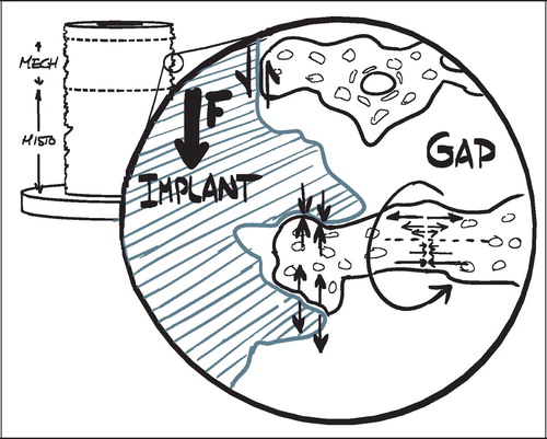
Implant model

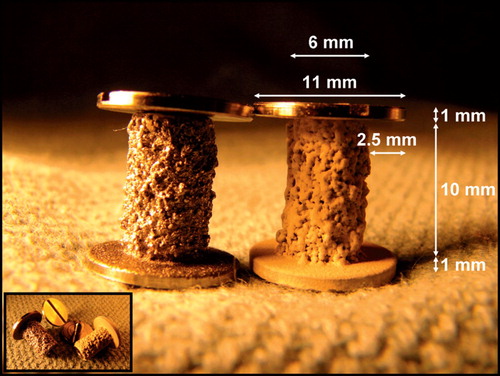
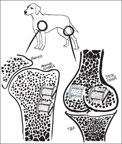
The employed implant model was based on an established model developed by Kjeld Søballe (87) and designed to study early fixation and osseointegration of an uncemented implant component inserted into a bed of impacted graft material (43;58). The implants consisted of a cylindrical plasma spray porous‐coated titanium implant body of 6 mm diameter with an 11 mm end disc mounted on each pole of the cylinder (Figure 2). The implant was implanted into an 11 mm diameter drill hole of 12 mm depth. The profound end disc secured concentric placement of the implant in the drill hole, by which it was surrounded by a 2.5 mm coaxial defect. This defect was packed with bone graft material. Containment was secured with a superficial end disc.

Figure 2. Non‐coated and HA‐coated plasma spray porous Ti implants with a 2.5 mm gap

All implants were inserted into the trabecular bone of the metaphyseal portion of long bones. In studies I and III each animal received four implants in the proximal humeri (Figure 3) with a centre‐to‐centre distance between neighbouring implants of 17 mm. In study II, the four implants were placed in the epicondyles of the distal femurs (Figure 3). The drill holes were made with cannulated drill bits at a rotational speed of lass than 2 rps to avoid thermal damage to the bone, and over guide wires placed with the aid of wire guides to secure uniform placement and standardized distance between implants.

Figure 3. Implant sites

The simplicity of this basic implant model makes it highly reproducible, and it yields less biological variance than inherent in a weight‐bearing model (87). The model also allows paired comparison of four treatment groups, and it permits a defect around the implant large enough for simulating impaction grafting. The trade‐off for its high degree of variable control is an absence of clinically relevant influences such as direct load transmission and joint fluid. Furthermore, the baseline healing capacity and remodelling rate of a dog is much larger than that of a human (17). It does not provide the revision environment of compromised bone as replicated in the micromotion model of Bechtold and Soballe (11). The animals were young, healthy and without any of the typical features of the ageing, often osteopenic skeletal changes that characterize the typical human recipient of a joint replacement.

Implant characteristics

All implants in studies I‐III were cylindrical, 6 mm in diameter and 10 mm in length. They were produced from a cylindrical titanium alloy (Ti‐6Al‐4V) core with a diameter of 4.4 mm, onto which a 1.3 mm closed porous Ti alloy coating was added by plasma spray technique (Biomet Inc., Warsaw, IN, USA). In study I half of the implants were further added a 50 μm hydroxyapatite (HA) coating by plasma spray technique through the same vendor. Both the plasma spray Ti coating and the HA coating are the same employed on clinical implants from the same manufacturer, and represented a clinically relevant, standard surface coating for uncemented implants. The surface characteristics of equivalent implants have been measured previously, and were not repeated for the implants in the studies I‐III. The Ti plasma spray coating technique provided an average gross surface roughness (R_a) of 47 μm, with a maximum peak‐to‐peak profile amplitude (P_t) of 496 μm. When the HA‐coating was plasma‐sprayed onto this surface, roughness and peak‐to‐peak amplitude were reduced to 41 μm (R_a) and 445 μm (P_t), respectively (87).

In studies II and III the implants served as substrates for other interventions. This was largely also the case in study I, but in this study the implant surface also served as an independent variable in the unpaired comparison between non‐coated and HA‐coated porous Ti implants. According to the previous roughness‐measurements, the addition of an HA‐coating by plasma spray technique introduces changes to the gross surface roughness. This could also be seen on the implants (Figure 2). The implants were randomly selected for HA‐coating. Whereas the HA coating thickness added to the implant diameter, the coating procedure by plasma spray technique to some extent smoothened the porous Ti substrate surface, whereby the implant diameter was in fact slightly reduced (p=0.06) (Table 1). The reduction in gross roughness and porosity of the HA‐coated implants was regarded as relatively small, and a potential impact on implant fixation was presumed to be opposite of the expected benefit of the HA coating. This was not further explored.

Table 1.  Mechanical specimens' diameter and height

Study		Diameter		Height
		mean	(sd)	mean	(sd)
I	all	5.69	0.24	3.29	0.33
	Ti	5.75	0.25
	HA	5.63	0.22
II	Ti	5.74	0.20	3.24	0.21
III	Ti	5.96	0.18	3.11	0.32

The cylindrical design of the implants offered the advantage of uncomplicated and highly reproducible surgery. The implantation site was a simple drill hole created by cannulated drilling. The initial guide wire was placed perpendicular to the bone surface, and this served as axis of revolution for the cannulated drill bit and was identical to the natural vertical axis of the implant. A uniform placement of the neighbouring implant was secured with a wire guide. The cylindrical shape was advantageous in the subsequent specimen preparation, and in the mechanical and histomorphometrical analysis.

Specimen preparation

In each of the studies I‐III the animals were killed after four weeks observation time with an overdose of hypersaturated barbiturate. The proximal humeri and distal femora were harvested and stored at −20°C for about one week pending preparation. At preparation, the bone‐implant specimens were thawed, and the implant's cortical endcap was exposed and unscrewed. The specimens were mounted by their diaphysis in the sliding holder of the water‐cooled Exakt^® diamond band saw and the implant aligned visually for transverse sections with the aid of a 10 cm long light‐metal threaded pin mounted in the implant's female thread for the removed cortical endcap. The outermost 0.5 mm was sectioned off and discarded. The next 3.5 mm of the implant was sectioned off and refrozen at −20°C pending mechanical testing. The remaining profound part of the implant was fixed in 70% ethanol pending further preparation for histology (Figure 4).

Figure 4. Transverse section for mechanical testing

Mechanical testing

The implants were tested to failure by push‐out test on an Instron Universal Test Machine (Model 4302, Instron, UK). Testing was performed on the 3.5 mm transverse section of the outer part of the bone‐implant specimens (Figure 4). The section was placed with the superficial/cortical side up under a flat‐faced cylindrical probe of 5.0 mm diameter on a support jig with a 7.4 mm opening, by which the clearance to the implant edges was about 0.7 mm as recommended by Dhert et al (16). Testing was performed blinded and in one session (32). Probe‐implant contact was defined by a 2N preload, after which testing started. The probe was advanced by 5 mm/min, and the load‐displacement data points were recorded every 10 μm and transferred to a PC. The probe speed was chosen as relatively low to reduce the viscous component of deformation and thereby increase testing sensitivity.

Test parameters

The implants had varying diameters, and the sections for mechanical testing had varying heights (Table 1). To aid comparability, the load‐data were normalized by an approximation of the surface area (implant diameter×height×π). Three parameters were calculated from the force‐displacement curves:

• Ultimate shear strength [MPa],

• Apparent shear stiffness [MPa/mm]

• Energy absorption [kJ/m²].

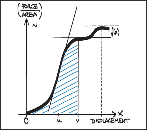
Ultimate shear strength (Strength, S) was defined as the value at the first peak of the normalized force‐displacement curve (Figure 5). This was also considered the point of implant failure. Later peaks occurred (Figure 6), but were regarded as post‐failure interlocks and not included.

Figure 5. Force‐displacement curve (normalized)

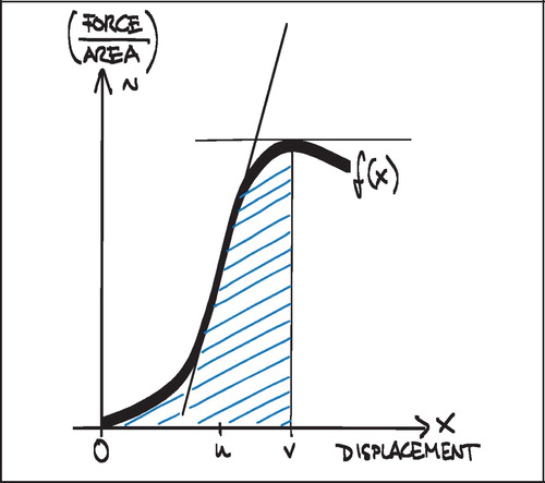
Figure 6. Force‐displacement curve with two peaks

Apparent shear stiffness (Stiffness) was defined as the maximum slope of the normalized force‐displacement curve before failure (Figure 5):

Energy absorption (Energy) was defined as the area under the curve of the normalized force‐displacement curve before failure (Figure 5).

Since the measurements were data points and not represented as an algebraic equation, the calculations were autogenerated in a spreadsheet (Microsoft Excel). The first peak was identified by the first negative inclination of a line between five successive data points on the curve, yielding Strength. Next, the largest slope between five successive data points on the curve was identified between zero and the displacement value for the first peak. Finally, the area under the curve between zero and the displacement value for the first peak was approximated by:

By the applied push‐out test only the force needed to maintain the implant displacement rate is measured. As the implant is pushed out of the surrounding bone, increasing force is applied, and a multiplicity of material stresses can be imagined transmitted into the tissue in which the implant is anchored. At tissue‐implant interfaces parallel to the axis there will be shear forces, on tissue inter‐digitating with the implant porosity there will be compressive and tension forces, and these forces may be transmitted outwards along radiating tissue structures as bending and torsional forces (Figure 7).

Figure 7. Force and material stress multiplicity at the bone‐implant interface at axial push‐out test

No reproducibility measurements were conducted on the mechanical datasets, since the three parameters were autogenerated by defined algorithms.

Failure interface

The surface of all implant sections was examined visually after the push‐out test. Except within the deep pores, there was macroscopically no tissue left on the implant surface of the uncoated porous Ti implants, and small islets of calcified tissue on most of the HA‐coated implants. There was no delamination of the porous Ti coating nor the HA‐coating. The failure site of the implants was therefore regarded as the bone‐implant interface for all implants, but there was a risk of underestimating the Strength parameter on the HA‐coated. The multiple interfaces within the grafted coaxial defect and the graft‐drill hole interface were not evaluated.

Interpretation of the mechanical test

The three mechanical test parameters, Strength, Stiffness and Energy as defined above, are all obtained from the normalized force‐displacement curves. These parameters supplement each other and represent different aspects of the mechanical implant fixation, and have been shown to correlate well with what is thought to be desirable histological implant fixation (87).

The Strength parameter reflects the normalized force necessary to induce failure of the bone‐implant interface. This may not seem to be a clinically relevant parameter, as most clinical implants are not assumed to fail due to single exposure of very high forces, but rather repetitive exposure to lower forces. Implant subsidence may reflect repetitive failures and implant resetting in the early phase of bone‐implant healing. This may advocate the Strength parameter as an important target for early improvement.

The Stiffness parameter may be interpreted as a measurement of the rigidness with which the implant is anchored in the surrounding tissue. Increasing Stiffness indicates a high deformation resistance, but may also indicate that the anchorage is more brittle. A low Stiffness indicates anchorage in a tissue construct with a lower deformation resistance and perhaps also higher ductility. High Stiffness values may therefore be indicative of fixation in calcified tissue, and low Stiffness values indicative of fibrous tissue encapsulation. Although cyclic testing within the limits of elastic deformation was not performed, the range of implant micromotion would be inversely related to the Stiffness value for a given applied force within the elastic force range.

The Energy parameter is positively related to Strength, but may be inversely related to Stiffness (69). This means that high values can be obtained at very different fixation scenarios, and it should therefore be interpreted with care. The ability of a particular tissue to absorb energy may be an important characteristic that is analogous to its resilience and toughness. However, the implants are anchored in different tissues and tissue combinations, and the difference in ability to absorb energy between tissues may not necessarily reflect the suitability of a tissue for implant fixation.

The focus of studies I‐III was the relative change in test parameters between groups rather than the absolute values.

Mechanical test considerations

The push‐out test only considers load in the axial direction, but torsional forces are presumed to have great influence on clinical joint replacements and the femoral component of the hip arthroplasty in particular. Given the simplicity of the applied implant model, it seems that the application of torsional forces would only redirect the force multiplicity by π/2. This may give a different absolute outcome of the tests, but is not likely to influence relative differences between the paired implants, or to be particularly applicable to subsegments of clinical forces.

The push‐out test is in its nature destructive, meaning that the transverse section of a specimen being evaluated mechanically cannot be evaluated by histomorphometry. Histomorphometry is performed on a transverse section below (Figure 7). The interpretation of both datasets assumes a relative comparability between the two sections that seems fair, but hardly accurate. A non‐destructive test could permit the mechanical and histomorphometrical parameters to be obtained from the same section of the individual specimen. It could also permit a more detailed analysis of the viscoelatic properties of the bone‐implant interface after preconditioning, which may be a useful target for intervention in terms of clinical relevance. A repetitive non‐destructive test of cyclic loading within the forces of viscoelastic deformation is currently being developed for the model (Figure 8).

Figure 8. Schematics of cyclic test and push‐out

One challenge of non‐destructive testing is obviously determining the range of the cyclic forces, to ensure that the forces do not inflict plastic deformation. This can be particularly challenging in studies with large differences between the groups.

Histomorphometry

The histological specimens were dehydrated in graded ethanol 70–98% containing 0.4% basic fuchsine and then embedded in methyl methacrylate (MMA) in a cylindrical mould with the implant's and mould's natural vertical axes parallel. After random rotation around its vertical axis the implant was sectioned parallel and about 1 mm offset to its vertical axis using a microtome (KDG‐95, MeProTech, the Netherlands). Four to five serial vertical sections were then obtained from the central part of the implant. The sections were 20–30 μm thick. For each section cut, about 400 μm was lost to the saw blade, giving the distance between each serially cut section.

During the microtome sectioning, the specimens were counterstained with 2% Light Green for two minutes. This stained the mineralized tissue exposed by the microtome in the cross‐sectional plane. Although its penetration depth was about 5–10 μm (70), bone below the cross‐sectional plane was protected from staining by the MMA, and the stain provided a standardized optical focus plane for light microscopy independent of potential variations in section thickness. The infiltration of basic fuchsine had already stained collagen and cell components including nucleic molecules red.

Histomorphometry was performed using a light microscope (10x/0.40), and the tissues were divided into five types based on their morphological appearance: bone graft, new bone, fibrous tissue, marrow space and unknown tissue. Bone was stained green, and therefore easy to distinguish from the other tissues. The bone graft was assumed to be lamellar bone, with the typical highly organized lamellas and lamella‐oriented stretched‐out oval cell lacunae without nucleic material. Newly formed bone was assumed to be immature woven bone, appearing less organized with larger, round cell lacunae containing nucleic material and chromatin. When ceramic bone graft substitute was used, this appeared brown and was easily distinguishable from the organic tissues. The ceramic granules were sometimes infiltrated by newly formed bone. This was classified in a separate category, and the counts were divided equally between the bone graft category and the new bone category at analysis. Fibrous tissue was identified by its presence of clearly visible fibril fibre complexes and low cell density. Generally, the fibrous tissue largely appeared oriented, dense and well‐organized, but it was also seen as a loosely, not clearly oriented, interconnected fibrous network. Marrow space consisted of fat vacuoles and surrounding blood cells, many of which were polymorphonuclear. Less than 1% of the counts were recorded as unknown, of which some were cartilage and some artifacts. The number was so low that is was taken out of the final analysis and statistical evaluation.

During the histomorphometrical analysis, the specimens were blinded to the examiner, although blinding was not possible for the discrimination between HA‐coated and non‐coated implants or between allogenic bone graft and ceramic bone graft substitute.

Stereological histomorphometry

Volume fractions of tissue surrounding an implant or area fractions of tissue covering the surface of an implant are quantities occurring in 3D. The histological sections are, however, 2D, and estimates of the geometrical parameters in 3D space must be made from these 2D sections. Stereology is a methodology that relates geometrical parameters such as volume and surface area of spatial objects to lower dimensional measurements obtainable on sections of the object. In short, stereology is the science of three‐dimensional interpretation of flat images.

Parameters such as volume and surface have profiles on 2D sections that can be quantified with the frequency of intersections between a parameter and a test probe superimposed into the section. A prerequisite for attaining unbiased estimates of these parameters is that the sum of dimensions in the probe and the parameter must be at least three. A second prerequisite is that the likelihood of intersection between a parameter and a test probe is independent of orientation in space.

Volume fractions are 3D and must be measured by 0D or higher probes, for instance the 0D probe of point counting. The relation for estimating volume fractions by point counting is VV=V(obj)/V(ref) equal to the PP=P(obj)/P(ref). PP is the fraction of points on a randomly positioned systematic point grid hitting the object (or tissue) of interest. Since the point counting probe is dimensionless, estimates of volume fractions are always orientation independent, and require no assumptions on isotropy and tissue or probe orientation in space.

Analogous to this, surface fractions are 2D and must be measured by 1D or higher probes. We used a line‐intercept technique (1D), in which sine weighted grid lines are randomly superimposed onto the section. Whenever a line probe intersects the implant surface, the tissue in the intersection is classified and recorded. Whereas estimates of volume are orientation independent, isotropy of either the material or the sections of the material is a requirement for estimates of surface. A very rough or a very flat surface of a cylindrical object can usually be regarded as isotropic, although the claim of perfect isotropy for most rough surfaces may be questionable. The implant surfaces were therefore regarded as being potentially anisotropic, and sine weighted grid lines were applied accordingly.

The vertical sectioning technique allows isotropic uniform random (IUR) sampling in 3D space of anisotropic materials without assumptions on the nature of the anisotropy. The technique was first described by Baddeley et al. (8) and involves the following four requirements: 1) an identifiable vertical axis, 2) sections parallel to the vertical axis, 3) sections placed after random rotation around the vertical axis and, 4) orientation of the test lines being weighted proportionally to the sine of the angle between the test line and the vertical axis. The first three requirements generate vertical uniform random (VUR) sections. The fourth requirement of sine weighted lines ensures that the test lines are IUR in 3D space (Figure 9).

Figure 9. Vertical sectioning technique

Stereological design of studies I‐III

The sections of the present studies were designed to fulfill the requirements of the vertical sectioning technique. Sections were made after random rotation around and cut parallel to the easily identifiable vertical axis of the implant, and the 1D line probes for surface estimation were sine weighted. To achieve a relatively uniform angle between the section plane and the implant surface, as well as minimizing distortion of the apparent width of the coaxial, grafted defect around the implant, the sections were taken from the central part of the implant (Figure 10). By doing this, only a preselected few of many possible sections were available for histomorphometry, and sampling was therefore not uniformly random. This gave sources of bias which will be discussed in the next chapters.

Figure 10. Exhaustive vertical sections (above) and central vertical sections (below)

Determining regions of interest

Two regions of interest (ROI) were defined: A Zone 1 of the immediate implant vicinity and a Zone 2 of the grafted gap surrounding the implant. Given the irregular nature of the rough titanium surface of the implants, it was found impractical to define ROIs that extended a predefined distance from the implant surface at any given point. Instead, an approximated surface line was defined as the line between the innermost “fjord” and the outermost “isle” of the implant coating profile on the sections (Figure 11). This approximated surface line acted as a reference from which the extent of the regions into the tissue around the implant was defined. Zone 1 extended 0.5 mm outwards into the surrounding tissue from this reference line, but also inwards including the solid implant and therefore all implant porosity central of the reference line. Zone 2 was defined as 0.5–2 mm from the reference line (Figure 23). This definition of Zone 2 ensured that sampling occurred within the drill hole for all implants.

Figure 11. ROI reference line (”approximated surface line”) for placement of Zones 1 and 2

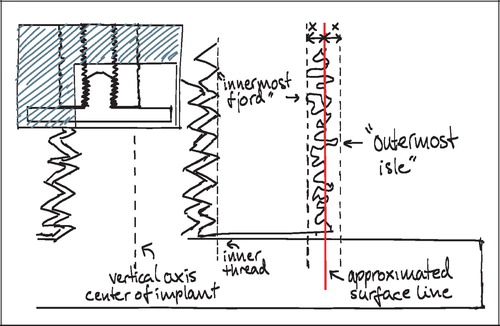
Other options were considered, but it was found that this gave the highest reproducibility of the ROIs, given a possible variation in porosity and coating thickness. The innermost fjord or the outermost isle could also act as starting origin for the zones, but the zone offset due to porosity differences would potentially increase by a factor two compared to the described approximated surface line. More central reference lines such as the implant center or the core implant‐coating interface could also have served as reference lines, but were not well defined in the sections. The inner thread of the implant was well defined, but as would be the case with increasingly central points of reference within the implant, it was found to be too sensitive to the individual section's offset from the vertical axis (Figure 12).

Figure 12. Section offset

Section offset bias

The regions of interest described above were defined under the assumption that the sections could be viewed as not only being parallel to the vertical axis of the implant, but also that the section was central so that the vertical implant axis actually lay within the section plane. This was not the case. Four to five central sections per implant were cut parallel to the vertical implant axis as described above. Each section was about 30–50 μm thick, but another 390–400 μm was lost to the blade of the microtome in the process of sectioning. Therefore, the section offset from the implant axis could be up to 1 mm for the most peripheral section.

It is obvious, that such an offset affects the comparability of predefined ROIs between different sections. A near‐tangential section through the very periphery of an implant will appear to have a smaller implant diameter, thicker implant coating, and a wider drill hole defect around the implant than a section through the center of the same implant (Figure 12).

Whereas a predefined ROI may cover a coaxial defect around an implant to a certain extent in a central section, the defect will be covered to a lesser extent by the same ROI on a peripheral section. Since the starting point of the zones is defined from the implant surface as described above (Figure 11), the zone will not reach as far into the periimplant defect on a peripheral section as on a central section. This gives a systematic difference between sections in terms of which parts of the periimplant defect that has actually been sampled. The question is then, to which extent there is a systematic difference, and which parameters are affected by it.

The apparent geometric differences between the vertical sections can easily be calculated as a function of the offset of a section from the vertical axis. On a transverse section, the implant is seen as a circle with a radius s enclosed by the circular profile of the drill hole with a radius t, where g = t‐s is the width of the coaxial gap defect around the implant. The profile of a vertical section will be viewed as a line through the transverse section.

A vertical section with an offset x from the vertical axis of the implant will have an apparent implant radius, and apparent drill hole radius tˆ and an apparent gap width. The Pythagorean theorem gives the following relation between the apparent gap width and the section's offset x from the vertical axis:

In the most peripheral section of a ø6 mm implant in a ø11 mm drill hole with a maximum offset x = 1 mm, the implant radius would appear to be 2.83 mm instead of 3 mm (a 5.7% decrease), and the gap width would appear to be 2.58 mm instead of 2.5 mm (a 3.2% increase).

In short, central sections are sampled from a ROI reaching further out into the grafted defect than in more peripheral sections. Whether or not the tissue parameters are affected by this depends on the homogeneity of the tissues along the axes radiating out from the vertical axis. If the representation of a specific tissue at a specific location is independent of the distance from the implant surface towards the drill hole border, then this represents no problem. This is, however, not a fair assumption in the present implant model.

In the applied gap model, neovascularization and recruitment of osteoprogenitor cells can be expected to originate from the vital trabecular bone beyond the drill hole border. In the parts of the gap close to the drill hole border one could expect a more progressed stage of bone metabolism with perhaps more newly formed bone, less allograft and less fibrous tissue, compared to parts of the gap close to the implant. All tissue parameters are expected to be affected by the described systematic sampling difference between the sections.

A solution to the section offset bias could have been dynamic, offset‐corrected regions of interest in the sampling. However, since the impact on the apparent gap width was only a 3.2% increase, it was considered to be of negligible importance. Furthermore, since this source of bias occurred within the sections of the individual implant, and since the data from the sections of an implant were pooled, there was little suggesting that this could systematically influence the relative differences of tissue fractions between implants.

Central section bias

The grafted defect surrounding the implants could be viewed as a coaxial lining of a cylinder. The inner perimeter P_inner of such a coaxial liner is obviously smaller than the outer perimeter, P_outer, and this relationship is defined by the outer radius t and the inner radius s of the lining:

For vertical sections close to the vertical axis, points counted close to the implant surface represent smaller volumes of tissue than points counted in the gap far away from the implant (Figure 13). Correspondingly, surface line intersections within the deep pores of the implant (close to the vertical axis) represent a smaller area than surface intersections recorded on protruding parts of the porous coating (far from the vertical axis).

Figure 13. Central section point representation of coaxial volumes

This means that the likelihood of a structure appearing in a central vertical section decreases with increasing distance from the vertical axis (Figure 15). This would not be a problem for exhaustive serial sections parallel to the vertical axis of the entire implant‐gap complex. Here, the under‐representation of distant tissue on central sections would be compensated by an over‐representation of distant tissues in more peripheral and near‐tangential sections.

Figure 15. Transverse section of implant (left) and objects with increasing distance to vertical axis

In the present studies, we sampled from serial sections parallel to the vertical axis from the central part of the implant (Figure 10). It must therefore be assumed, that tissue fractions near the implant are overrepresented compared to tissue fractions far away from the implant. This would not be a problem if one could assume relative tissue homogeneity along the axes radiating out from the vertical axis. But, as discussed above, this does not seem like a fair assumption in the present studies.

The phenomenon of over‐representation of parameters located close to the implant versus distant ones is also known from FAVER (Fixed Axis Vertically Rotated) sections. Unlike in a VUR section, the vertical axis always appears in a FAVER section, meaning that a true FAVER section is not only cut parallel to the vertical axis but through it (Figure 14). It is, in other words, the most central VUR section. As suggested by Balatsouka et al. (9), this bias can be counteracted by weighting each probe count by its distance to the vertical axis. Such weighting was not performed in the present studies, and it must therefore be assumed that the data are indeed biased.

Figure 14. FAVER sections

A necessary discussion

With the use of sample recounts we will show that this bias has a rather small influence on the histomorphometrical results reported in the studies I‐III (Table 2). However, in order to give a satisfactory scientific justification of the presented data, it is necessary to undertake a mathematical discussion of it. The model and methodology have been in use for many years. The bias' influence on the data is highly dependent on the model, the data sampling and the tissue distribution on and around the implant. This generalization of the bias may aid in the justification of previous data as well as outline the methodology that could be applied in future studies.

Table 2.  Influence of central section bias on sample tissue volume fraction estimates in Zones B+C+D = Zone 2 (3.5–5 mm). V_VUR: Non‐weighted tissue fraction. V_FAV: distance‐weighted tissue fraction. V/V= V_VUR/ V_FAV

Implant	Bone graft			New bone			Marrow space			Fibrous tissue
	VVUR	VFAV	V/V	VVUR	VFAV	V/V	VVUR	VFAV	V/V	VVUR	VFAV	V/V
1	23.3%	23.1%	1.01	25.9%	26.0%	0.99	50.8%	50.9%	1.00	0.0%	0.0%	‐
2	39.1%	39.6%	0.99	31.3%	31.1%	1.01	29.6%	29.3%	1.01	0.0%	0.0%	‐
3	32.0%	31.8%	1.01	23.8%	24.0%	0.99	44.2%	44.2%	1.00	0.0%	0.0%	‐
4	39.4%	39.2%	1.01	18.4%	18.6%	0.99	42.2%	42.3%	1.00	0.0%	0.0%	‐

Central section bias model I: The basics

To understand the impact of the central section bias, it is helpful to generalize the relationship between tissue representation and distance from the vertical axis. As stated previously, VV=V(obj)/V(ref) is equal to the PP=P(obj)/P(ref) in VUR sections. The relative representation of a tissue P(obj)/P(ref) on a section can be expressed as a function of the distance from the vertical axis, f_T (r) (Figure 16). The relative representation of all tissues P(ref)/ P(ref) can also be expressed as a function of the distance from the vertical axis f_TOT (r), but it is independent of r and equal to 1 (Figure 17).

Figure 16. Relative tissue representation as a function of distance from the vertical axis, f_T (r)

Figure 17. Relative total tissue representation as a function of distance from the vertical axis, f_TOT (r)

In VUR sections the relative volumetric representation of a tissue V_T in a region of interest s to t mm from the vertical axis would be:

In FAVER sections, the equivalent relative volumetric representation of a tissue V_T in a region of interest s to t mm from the vertical axis would have to be weighted by the distance to the vertical axis:

The ratio V_T(VUR) / V_T(FAVER) expresses the misrepresentation of a tissue fraction V_T on a FAVER section evaluated as a VUR section where the counts were not weighted with the distance from the vertical axis:

A simple mathematical interpretation of Eq 8 is, that the V_T(VUR) / V_T(FAVER) ratio is the same as the ratio between the r‐coordinates of the geometric centroid (GC, also gravitational centre) for the relative representation of all tissues TOT (equivalent to the ROI) and the geometric centroid of the relative representation of a specific tissue T within the ROI:

Since the r‐coordinate of the geometric centroid for the rectangular ROI is always ½(t + s) the V_T(VUR)/V_T(FAVER) ratio depends on whether the geometric centroid of the tissue representation T lies to the left or the right of ½(t + s. If the geometric centroid of the tissue representation T is to the right of ½(t + s), then the V_T(VUR)/V_T(FAVER) ratio will be smaller than 1, indicating an underestimation. If the geometric centroid of the tissue representation T is to the left of ½(t + s), then the V_T(VUR)/V_T(FAVER) ratio will be larger than 1, indicating an overestimation (Figure 18). This will be shown more specifically in the following models of the bias' influence.

Figure 18. Different geometric centroid for all tissues TOT and a specific tissue T. The area A_TOT, has a gravitational centre in the symmetry line of the ROI; r = ½(t + s). Because of the skew tissue distribution of T, the area A_T, has a gravitational centre to the right of r = ½(t + s.

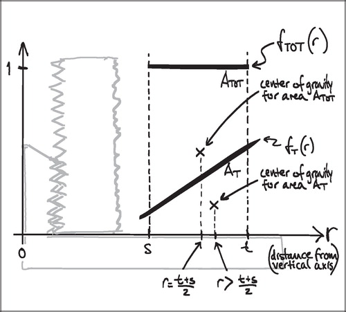
Central section bias model II: The extremes

To explore the boundaries of the V_T(VUR) / V_T(FAVER) ratio, it is helpful to consider situations of maximal tissue inhomogeneity. This can most easily be expressed by a discontinuous step‐function of the tissue distribution of a tissue T:

As Δs approaches zero, the tissue fraction f_T(r) of a particular tissue T becomes 1 at r = s, and 0 at s < r≤t. This means that the tissue T has full representation in an infinitely small portion of the implant‐near part of the ROI and is absent elsewhere. This extremely polarized distribution provides the upper limit of the V_T(VUR) / V_T(FAVER) ratio:

Equivalently; when a particular tissue covers the far end of the ROI and is absent elsewhere, the step‐function of that tissue distribution becomes

As Δt approaches zero, the lower limit of the V_T(VUR)/V_T(FAVER) ratio is reached:

This means that tissue fractions on a FAVER section of the implants evaluated as being VUR could be between 8% higher and 7% lower than the true value in a ROI equivalent to Zone 1, and between 21% higher and 15% lower than the true value in a ROI equivalent to Zone 2 in the present studies. This represents the greatest possible influence of the bias, occurring at infinitely small tissue fractions that are distributed completely inhomogeneously.

From these expressions it becomes clear, that increasing representation of a given tissue T within a ROI decreases the influence of the bias. This is simply due to that fact that the geometric centroid of an increasingly large area at either end of the ROI will approach the geometric centroid of the ROI itself (on the r‐axis).

If one continues to assume a completely polarized tissue distribution as described above, then x = Δs /(t + s) expresses the fraction of the ROI width measured outwards from the implant which is covered by the tissue T. By substitution of Δs = x ·(t−s) into (Eq 10) we get:

Equivalently for the fraction of the ROI width which is covered by the tissue T measured inwards from the outer perimeter of the ROI:

These two expressions (Eq 13, Eq 14) give the V_T(vur)/V_T(FAVER) ratio for any given representation x of a tissue T within a ROI under the worst possible tissue distribution within the ROI.

The tissue distribution across a ROI has a high influence on the impact of the bias. According to the second theorem of Pappus the volume of a solid generated by rotating a plane figure about an external axis is equal to the product of the area of the plane figure and the distance traveled by its geometric centroid (Figure 19). The geometric centroid of a ROI as defined above is ½(t + s). This means, that only the portion of a tissue fraction that is not distributed symmetrically around r = ½(t + s) is affected by the bias (Figure 20). Since most tissues in the ROIs of the current implant model are in fact represented on both sides of the ROI midline r = ½(t + s), the influence of the bias will be substantially smaller than in the situations described above.

Figure 19. Volume of torus: A×2πr

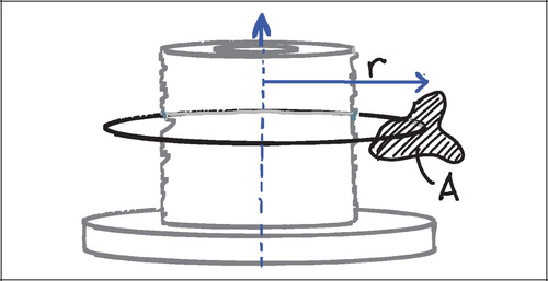
Figure 20. Example of distance‐dependent tissue representation symmetrical around r = ½(t + s)

Central section bias model III: The reality?

Realistically, tissues in the periimplanteric space of the current studies are represented with higher fractions of the total, and with a more homogeneous distribution than in the scenarios outlined above. The tissue representation can indeed depend on the distance from the vertical axis, but it is typically represented to some extent throughout the entire ROI (Figure 21).

Figure 21. Relative tissue representation as a function of distance from the vertical axis, f_T(r).

As an approximation of the distance‐dependent relative tissue representation, f_T (r), it seems fair to assume a linear relationship between the representation of a particular tissue T and the distance r from the vertical axis, f_T (r) = a × r + b. If a ROI is defined between the distance s and t from the implant's vertical axis and the relative tissue representation f_T (r) of a tissue T was known at the implant‐near and the implant‐far end of the ROI, then:

When Eq 15 is entered into Eq 8 the V_T(VUR) / V_T(FAVER) ratio can be expressed by:

Substitution (Eq 16) is performed for:

yielding the expression:

For Zone 1 (s=3; t=3.5) and Zone 2 (s=3.5; t=5) in the studies I‐III the expression becomes:

Central section bias trends

Based on the models described, the following general trends of the bias can be established:

• A tissue represented without dependency on distance from the vertical axis will be represented without bias.

• A tissue represented decreasingly with distance from the vertical axis will be overrepresented.

• A tissue represented increasingly with distance from the vertical axis will be underrepresented.

• Only the net distance‐dependent change between two symmetrical halves of the ROI is subject to bias.

The following tissue‐specific trends of the bias can be assumed for a bone‐grafted defect around an implant based on gap healing experience:

• New bone underestimation. New bone is increasingly represented with increasing distance from the vertical axis

• Bone graft overestimation. Bone graft is decreasingly represented with increasing distance from the vertical axis

• Fibrous tissue overestimation.

Fibrous tissue is decreasingly represented with increasing distance from the vertical axis Given the assumptions about linearity and representation throughout the ROI, the following limits of the bias influence can be established from f (A, B)(Eq 19, Eq 20 and Figure 22):

• Tissue area or volume fractions may be overestimated by up to 2.5% with increasing tissue density towards the implant in Zone 1 (f (A, 0)).

• Tissue volume fractions may be overestimated by up to 6.3% with increasing tissue density towards the implant in Zone 2 (f (A, 0)).

• Tissue area or volume fractions may be underestimated by up to 2.6% with increasing tissue density away from the implant in Zone 1 (f (0, B)).

• Tissue volume fractions may be underestimated by up to 7.6% with increasing tissue density away from the implant in Zone 2 (f (0, B)).

Figure 22. Graphic representation of the V_T(VUR)/V_T(FAVER) ratio in Zone 1 and Zone 2 as a function of A and B (Eq 19 and Eq 20) under the assumptions of linearity and tissue representation throughout the ROI.

Figure 23. ROI Zones 1 (inner) and 2 (outer)

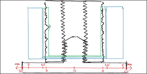
Central section bias and relative differences

The influence of the central section bias has been modelled on the tissue fractions within a single section. A median tissue fraction for the implant is determined from its four sections, and a median tissue fraction for the treatment group is determined from the implants in the group.

The influence of the central section bias remains the same throughout these steps, and holds true for the group medians reported in the studies I‐III. However, the main result of the studies is not how well or poorly an implant group is anchored in the surrounding bone, nor is it how small or large the fraction of newly formed bone or any other tissue is around an implant. The main focus of all studies is how these outcome parameters change under the influence of different variables.

The question is therefore, how the central section bias influences the relative difference in histomorphometrical parameters between the compared groups (here; estimated volume fractions of a specific tissue V_T in two intervention groups Group1 and Group2), expressed by:

The influence could be summed up in the following three scenarios for a tissue T:

1. The V_T(VUR) / V_T(FAVER) ratio for the compared treatment groups is the same.

   → No bias influence

2. The V_T(VUR) / V_T(FAVER) ratio differs between the compared treatment groups, but both are either larger than 1 or smaller than 1.

   → Bias' influence smaller than its maximal influence on the absolute tissue fractions.

3. The V_T(VUR) / V_T(FAVER) ratio is larger than 1 in one group and smaller than 1 in the other group.

   → Bias' influence larger than its maximal influence on the absolute tissue fractions.

It seems fair to assume that the main vector of a distant‐dependent change in representation of a specific tissue T remains the same for all groups. The magnitude of the change may vary between groups, as may also the level from which the change originates. This assumption corresponds to the second scenario above.

Testing the central bias influence

The mathematical modelling of the influence of the central section bias indicated that it could cause a systematic

• new bone underestimation by up to 2.6% in Zone 1 and 7.6% in Zone 2

• bone graft overestimation by up to 2.5% in Zone 1 and 6.3% in Zone 2

• fibrous tissue underestimation by up to 2.6% in Zone 1 and 7.6% in Zone 2

and that the estimate of relative differences between groups would be influenced, but to a lesser extent, and in any case within the limits of the bias' influence on the absolute fractions.

These bias influences were considered too low to warrant a data recount. However, it seemed appropriate to perform a small sample recount to ascertain the validity of the assumptions in the mathematical model of the central section bias.

Four random implants from study III were recounted (Figure 25). The gap was subdivided into five zones A‐E with 0.5 mm width, using the same approximated starting line near the implant as described previously (Figure 11). Zone A was therefore equivalent to Zone 1. Zones B‐C‐D were equivalent to Zone 2. Zone E was added to assess the influence of the section offset bias (Figure 24). Sampling intensity was the same for all Zones A‐E (mean 824 point counts per zone).

Figure 24. ROI Zones A, B, C, D and E

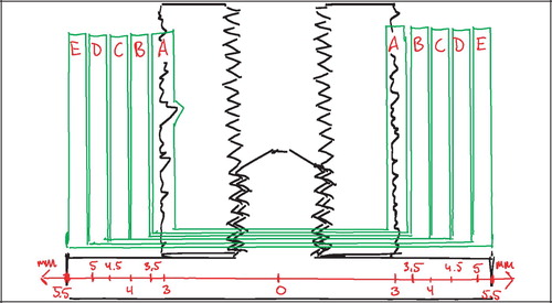
Figure 25. Tissue fractions (not weighted by distance to vertical axis) of the 0.5 mm Zones A‐E of the recount of four implants in study III.

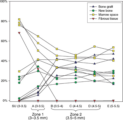
The sample recount confirmed that the model assumptions of linearity and tissue representation throughout the ROI (here Zone 2 = Zone B+C+D) were reasonable. It also indicated, that the outer limits of the bias influence would most likely not be reached, since the distance dependent tissue distribution was far more homogeneous than what was possible within the assumptions of the mathematical model (Figure 22, Figure 25).

The influence of the central section bias on the four recounted implants was expressed as the ratio between the applied non‐weighted tissue fraction estimates, V_T(VUR), and the distance‐weighted tissue fraction estimates, V_T(FAVER). Only Zone 2 (equivalent to Zones B‐C‐D) was considered, and the section offset bias was ignored. The V_T(VUR)/ V_T(FAVER) ratio was determined by:

P_T(B), P_T(C), P_T(D) are the points hitting a particular tissue T within the 0.5 mm Zones B, C, D at a mean distance r_B = 3.75 mm, r_C = 4.25 mm, r_D = 4.75 mm, and P_TOT(B), P_TOT(C), P_TOT(D) are the total number of points hitting a tissue within the 0.5 mm Zones B, C, D at a mean distance r_B = 3.75 mm, r_C = 4.25 mm, r_D = 4.75 mm (Figure 24).

The subdivision of zones into narrow segments was chosen over the more correct way of recording the distance between the vertical axis and the individual point or intersection counted. The software did not allow registration of the coordinates of the individual counts, and manual registration would be subject to typing‐errors.

The V_T(VUR)/V_T(FAVER) ratio was in the range 0.99–1.01 for all tissues in all recounted implants (Table 2), meaning that the impact of the bias was a systematic over‐ or underestimation of the tissue fractions of around 1%. The recounted sample was too small to provide general conclusions as to how each tissue fraction changes with increasing distance from the vertical axis. However, the theoretical trends of distance‐dependent increase of new bone and distance‐dependent decrease of bone graft were to some extent confirmed. The large distance‐dependent changes in tissue volume fractions seem to occur within Zone 1 (=Zone A), and especially for bone graft and fibrous tissue. Zone 1 includes the pores of the implant surface, which dead graft material cannot migrate into. The presence of fibrous tissue usually occurs as an encapsulation of the implant and is therefore largely to be found within Zone 1, which is the case in all studies I‐III.

Controlling section offset bias and central section bias

It has been established that the tissue fraction estimates in the studies are subject to systematic errors. The section offset bias is caused by a mismatch between the apparent size of the actual ROI and the sampling ROI, resulting in an underestimation of tissues that are increasingly represented in the implant‐far end of the ROI. The central section bias is caused by the use of central sections without weighting the counts with the distance from the vertical axis, thus overestimating tissues near the implant and under‐estimating tissues far from the implant.

The estimates of the bias influence indicate that it is within a range that is low and even negligible. This was verified by sample recounts, and it seems very unlikely that it has had any influence on the conclusions of studies I‐III. However, any systematic error in the data collection should be avoided, because such errors are difficult to manage after completion of data collection. In the case of section offset bias and central section bias, the systematic error is well defined.

To avoid these types of systematic errors in future studies, it is important to understand the limitations of the sections used. One challenge in studies I‐III is that the sections are somewhere between true VUR sections and true FAVER sections. In order to weight the counts correctly, the apparent distance from the vertical axis to each counting point should be corrected by the section's offset from the vertical axis before weighting is performed. When the offset is smaller than one‐third of the radius of the coaxial structure, as is the case in these studies, this correction may be negligible. However, both the ROI offset correction factor and the count weighting factor are defined by the offset and the distance to the vertical axis. With computerized sampling within a digitally defined ROI and with digitally superimposed probe grids, the coordinates of each probe count are well defined. User input would only be the section's offset and defining the vertical axis, and the correction could be generated automatically. As long as this algorithm is not available in the stereological software, an alternative solution would be to subdivide a coaxial volume projection into narrower zones, between which weighting could be performed, and within which the importance of weighting would be negligible.

Section thickness bias

Ideally, the sections for histomorphometry should be true 2D planes. This is not the case, as the sections had a thickness of around 30 μm. Thus these sections are five‐fold thicker than sections without implants cut on a classic microtome or cryostat, and introduces sources of bias due to over‐projection that need careful consideration.

Implant surface over‐projection

The shadow effect of the implant surface (9) is a well‐known problem in the relatively thick implant sections. The shadow effect occurs when an opaque structure is sectioned at an angle not normal to the surface of the structure. It causes the real interface between the two structures to be covered by the shadow of the opaque structure (Figure 26). The effect increases with section thickness and the deviation from a right angle.

Figure 26. Shadow effect

A certain degree of shadow effect must be expected on half of the implant's total profile length, and roughly 15% (½ × (1‐sinπ/4) ) of the total implant profile will cast a shadow equal to or larger than the section's thickness of about 20–30 μm. The implants have a highly irregular porous surface, and the angle between the implant surface and the section plane can be assumed to be between 0 and π, and symmetrical around π/2. Angles between 0 and π/2 will have decreasingly large shadow effect, whereas there will be no shadow effect on angles between π/2 and π. Since the implant surface can be regarded as near‐isotropic, the shadow effect occurs randomly within all sections and independent of the section's offset from the vertical axis.

There are two main problems related to the shadow effect in the present studies: 1) a decreased ability to determine what is in direct contact with the implant, and 2) a risk of underestimating thin tissue surface area fractions. The first problem is simply related to the fact that the very intimate implant surface perimetry is not visible in about half of the line probe‐implant intersections. Interposition of very thin micro‐structural layers between implant and the tissue recorded as adjacent to the implant cannot be excluded. The second problem is that it causes an underestimation of surface area fractions which are covered by a thin layer of a particular tissue. Since loose connective tissue may be more likely to form such a thin, interposing layer against the implant surface than calcified tissues, the shadow effect gives a risk of systematic overestimation of the new bone surface area fractions.

Tissue over‐projection

Tissue over‐projection mainly occurs at the interface between two tissues of different opacity, where the more opaque tissue will be over‐projected. This causes a systematic overestimation of the volume fraction of the more opaque tissue at the expense of the more transparent tissue. The phenomenon is directly related to section thickness and inversely related to the size of the tissue structure. This means that tissues that are fragmented into small isles are more prone to the phenomenon than tissues occurring as larger, more continuous structures. A rule of thumb is to aim for a section thickness that is less than one‐tenth of the height of the average 3D particle within the matrix being sectioned (36).

The problem of tissue over‐projection in studies I‐III mainly occurred within in the non‐calcified tissues, causing an overestimation of fibrous tissue and an equivalent underestimation of marrow space. These tissues were visualized by infiltrative basic fuchsin staining. Although the optical focus plane was that of the surface‐stained calcified tissues, this could not prevent some over‐projection from structures below the cross‐sectional plane. Since fibrous tissue is more opaque than the components of the marrow space, the projection of fibrous tissue onto the cross‐sectional plane was higher than the actual cross‐sectional area of fibrous tissue. The volume fractions of fibrous tissue have therefore been subject to systematic overestimation. In all studies I‐III, however, fibrous tissue had little fragmentation and was predominantly present as a relatively continuous tissue within Zone 1. This caused the profile of the fibrous tissue ‐ marrow space transition to be small relative to the cross‐sectional area of the tissues, and thus the fibrous tissue overestimation to be correspondingly small.

The calcified tissues were visualized by Light Green counterstaining on the cross‐sectional surface. The stain penetration depth is about 5–10μm (70), causing a systematic overestimation of volume fractions of calcified tissues at the expense of non‐calcified tissues. This overestimation was considered small, since the stain penetration depth was small compared to the average particle size of bone in the sections. Furthermore, the Light Green staining of bone was assumed to be complete, and only structures with bone morphology as well as staining were recorded as bone. Whereas this assumption was practical, it was not completely accurate. The real staining completeness could be 100% or less (but for apparent reasons not over 100%), most likely causing a systematic underestimation of calcified tissues. These counteracting biases have not been subject to estimates of their magnitude, and it is therefore impossible to determine whether the net result was an over‐ or underestimation of calcified tissue volume fractions.

Unstained bone was also sometimes projected onto the cross‐sectional plane, impairing classification of the actual tissue in the plane. In these cases, the probe count was recorded as the nearest identifiable non‐calcified tissue (fibrous tissue or marrow space).

Efficiency of systematic sampling

In contrast to modern digital image analysis in which volumetric or area fractions are quantified based on the entire region of interest, quantitative histomorphometry relies on analysis of a selection of observations within a region of interest. Sampling efficiency means minimizing the selection of observations at the different sampling levels under consideration of variance contribution. By careful planning, the sampling and thus workload can be reduced to a minimum without a large effect on the observed variance.

The observed variance in a dataset is the sum of the biological variance and the variance contribution from the inaccuracy of the methods of used to acquire data:

The biological variance component can be controlled in the study design, and the methodological variance component can be controlled with sampling methodology and intensity. The biological variance cannot be estimated directly, but because of the relation described above all variance components can be described as a fraction of the observed variance. As a rule of thumb, the adequate methodological variance contribution is between one fifth and one half of the observed variance (31):

When the methodological variance contribution is lower than this, further sampling will not contribute substantially to the observed variance because it is largely biological. The goal is therefore not to have a low absolute methodological variance, but to keep it within a certain size relative to the observed variance.

Section sampling efficiency

Overgaard et al. have previously optimized sampling on an implant model similar to the one used in the present studies. From a paired study in humans comparing HA‐ and FA‐coated implants, the HA‐coated implants from five of the patients were used to analyze the methodological variance contribution to the observed variance as a function of sampling intensity on the following hierarchy of sampling levels: section, side and field of view. The authors found that sampling from four instead of fourteen vertical sections had virtually no detectable effect on the observed variance (71).

Some care should be taken in extrapolating these results to the experimental set‐up of studies I‐III. The methodological study was performed on humans of 22–58 years age who may be expected to have a larger biological variation in trabecular bone quality (and therefore in osseointegrative ability) than 14 month old dogs. Also, the biological variation in an unpaired study is expected to be larger than between paired implants within the same subject, due to interindividual differences. Since the accepted contribution of methodological variance is relative to the observed variance (and thereby to the biological variance), the demands on the methodological accuracy is less when the biological variance is high, and conversely.

Another important consideration is the spacing between the serially cut VUR sections. In the methodological study of Overgaard et al, each implant was divided into 14 exhaustively cut serial VUR sections. When every fourth section was sampled, this would imply that each section would be almost 2 mm apart. This way, a much larger part of the implant circumference would be represented in the sections than with the currently applied methodology of cutting serial VUR sections from around the center vertical axis of the implant (Figure 27).

Figure 27. Reducing the amount of sections

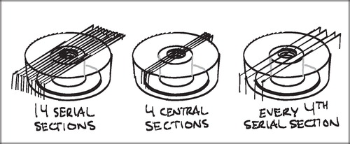
It is obvious that the spacing between sections can have an impact on how well the sections represent the implant circumference. If one considers the extreme case of ideal sections of 0 mm thickness, then four serial sections would be identical, and sampling all four would be equivalent to sampling one with four times the sampling intensity. When sampling from four two‐sided serial VUR sections around the center implant axis with a maximum X mm offset to each side of the center, the fraction of the circumference frC of an implant with I mm radius and a G mm gap width from which sampling commences will be:

For X = 1 mm, I = 3 mm and G = 2.5 mm the fraction of the circumference (frC) from which sampling occurs would be 21.6% for the implant and 11.6% from the drill hole border. This is certainly less than in the study from which the guidelines are derived. The maximum offset here would likely have been close to the implant radius, by which the whole implant circumference is subject to sampling. However; the guidelines from Overgaard et al. regarding the number of sections are still applicable to serial vertical sections around the center of the implant, provided a relatively homogeneous distribution of tissues around the grafted gap is present. This assumption seems fair; at least to the extent that relative homogeneity was assumed between 10–15% sectors of the implant surface and the grafted gap. In this context, it is not necessary to assume homogeneity of tissues in radiating distance from the implant, nor is it necessary to assume homogeneity of tissue fractions along the vertical axis (from superficial to profound). Such homogeneity is also very unlikely to be the case in this model due to the source and directionality of cellular recruitment and neovascularization in to the gap.

Tissue sampling efficiency

Sampling was based on four sections of each implant. Using the C.A.S.T.‐Grid software (Olympus Denmark A/S, Albertslund, Demark), the Zones 1 and 2 as described above were drawn and superimposed on both sides of the implant for each section. The meander sampling functionality was used. In each zone the sampling fraction was set to 100%, although only every other frame was sampled in Zone 2 of studies I and III. In each frame, 12 sine‐weighted line probes and 16 point probes were superimposed onto the image. In Zone 1, a median 535 line‐implant intersections and 490 point counts were recorded. In Zone 2 a median 1402 point counts were recorded in study I, 786 in study II and 825 in study III.

In order to plan efficient sampling, it is important to have some knowledge about the parameters subject to the sampling. The needed sampling intensity is related to the presence of the sampling object (a particular tissue) and to the difference in its presence between the groups compared. For instance, a highly represented tissue with a large difference between the groups can be sampled with a lower intensity than a rarely occurring tissue with a small difference in occurrence between the groups.

The sampling intensity was based on providing highly reproducible estimates of tissue fractions above 10%. The reliability of a tissue fraction estimate is obviously directly related to the number of point or line intersection counts on which the estimate is based. As a rule of thumb, such a tissue fraction estimate should be based on 100 counts (30); however much fewer counts can be acceptable if the differences between the groups is large. Based on these assumptions, the sampling was designed to record at least 500 counts per ROI per implant as described above.

Histomorphometrical reproducibility

Tissue classification is prone to error, because the distinction between tissues is not always absolutely clear. Furthermore, the histomorphometrical analysis takes place over a period of time, during which there is a risk that the examiner's distinction between two tissues may change.

These errors were sought reduced by defining the morphological tissue distinctions as clearly as possible and performing the histomorphometry over a minimized time period (less than one month). The time spent counting was viewed as an indicator of insecurity in the tissue classifications, and the ∼2000 counts made on the four slides of one implant were counted in 1–1½ hour efficient counting time (2–2.5 seconds per count). Prolonged counting time typically occurred for the first slides counted in a series; these were viewed as trial counts and recounted.

The histomorphometry was performed blinded and with implants in random order. Any change in the distinction between tissues over the course of the analysis would therefore be distributed randomly between the intervention groups and add to data variance rather than bias data.

If a null‐hypothesis of group equality is not rejected, then the groups do not differ, or the study has insufficient power to detect a difference that is actually there. In these cases, it can be of value to analyze methodological contributors to the total variance, such as reproducibility. If a large portion of the total variance can be attributed to poor ability to classify tissues (or insufficient sampling intensity), then this may have caused a Type II error. This is interesting, since methodological variance to some extent can be controlled, and is usually chosen to be higher than its potential minimum in order to reduce the histomorphometric workload.

In contrast, when a null‐hypothesis of group equality is rejected, this validates that the total data variance was within acceptable limits for the design and purpose of that particular study. It therefore also indicates that the reproducibility was acceptable. Analysis of variance contribution, including reproducibility measures, would not alter the main conclusion of the study, but rather indicate that the probability of falsely having rejected the null‐hypothesis (Type I error) could be even lower.

Measures of intra‐observer reproducibility were expressed as the within‐subject coefficient of variation (CV) calculated from double measurements of four randomly chosen implants from study III by the same examiner on identical equipment separated by two years by the expression:

where x¯ is the mean value of the first and the second measurement, k is the number of double estimates, and d is the difference between the first and the second measurements of the individual parameters (93).

The intra‐observer reproducibility was good and comparable to previous studies in this model (47). The within‐subject coefficient of variation decreases with higher tissue fractions because it does not only reflect the examiner's ability to reproduce tissue classifications, but also the sampling intensity. When the fraction of a particular tissue is low, the reproducibility of the equivalently small sample is low, and the relative impact of a tissue misclassification increases. This can be seen on the very high CV values calculated for the very small area fractions of bone graft on the implant surface and volume fractions of fibrous tissue in Zone 2 (Figure 28, Table 3).

Figure 28. Double counts of four implants

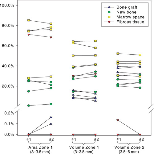
Table 3.  Histomorphometrical reproducibility (CV in percent)

	Bone graft	New bone	Marrow space	Fibrous tissue
Area Zone 1	206	12	3	6
Volume Zone 1	20	8	3	8
Volume Zone 2	4	4	1	283

Statistical analysis

The datasets were either paired with four groups (study I‐III) or unpaired with two groups (study I). The paired, multiple‐group datasets represented by normal distribution were evaluated with repeated measures ANOVA followed by paired t‐test. Datasets that where not normally distributed were evaluated with Friedman repeated measures analysis of variance by ranks followed by Wilcoxon signed‐rank test.

The unpaired dataset of the two implant surface groups (Ti and HA) were not represented by normal distribution and therefore evaluated with Wilcoxon rank‐sum test.

Many of the datasets were not represented by a normal distribution, even after logarithmic transformation. The histological datasets were evaluated non‐parametrically, as normal distribution could not be assumed for all parameters; in most cases because of values close to zero. Most the mechanical data followed a normal distribution and fulfilled the assumptions for parametric evaluation.

For all datasets, differences between the individual group means or medians were considered statistically significant for p‐values <0.05. Since four groups were compared, six tests were performed on each parameter. Such multiple testing increases the probability of the Type I error of falsely rejecting a true null hypothesis to 26.5% (1–0.95⁶). To counteract this “mass significance” problem, each parameter was tested under the null hypothesis of equality between all groups with repeated measures ANOVA or Friedman's test. Comparative tests between the individual groups were only performed if this hypothesis could be rejected with a p‐value < 0.05.

One dog was excluded from study III because it sustained a shaft fracture through the distal implantation site of the right proximal humerus two days postoperatively. No other exclusions were made in studies I‐III.

Statistical analysis was performed using Inter‐cooled STATA 9.0 software (StataCorp LP, College Station, TX, USA).

Summary of studies

All studies were done using the same non‐loaded experimental implant model surrounded by a 2.5 mm circumferential defect packed with graft material. The study design was paired and block‐randomized, and all analyses were blinded. The same sixteen dogs were used for studies I (shoulder) and II (knee), and another ten dogs were used for study III (shoulder).

The clinical objective was to improve fixation of uncemented implants where bone graft had been used as a void filler to provide mechanical support to the implant. For experimental purposes, such an improvement was defined as:

• improved mechanical fixation

• improved implant osseointegration

• increased new bone formation

• controlled allograft resorption

• decreased fibrous tissue formation

Figure 29. Overview of studies I‐III

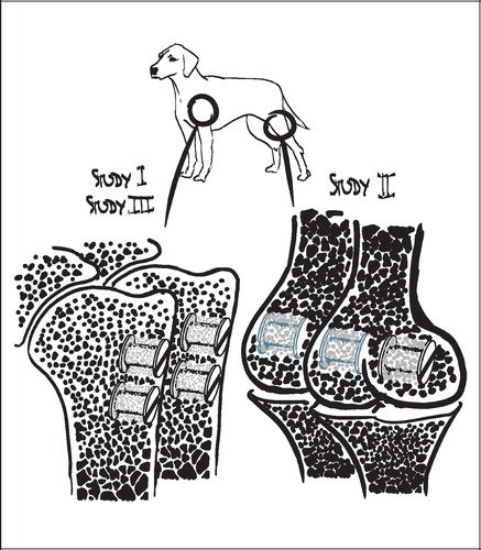
In the following overview tables, “0” indicates no change relative to the control, “+” indicates an improvement relative to the control and “−” indicates a deterioration relative to the control. The double signs “+ +” and “‐ −” indicate a group best or group worst.

Study I (Table 4)

Hypothesis 1: When rhBPM‐2 (BMP) and Pamidronate (BP) are added to allograft bone, early fixation of grafted implants is improved.

Table 4.  Change relative to control. “0”: no change. “+”: improvement. “−”: deterioration. The double signs “+ +” and “− −” indicate a group best or group worst

	Allograft treatment groups				Implant groups
	Control	BMP	BP	BMP + BP	Ti	HA
Mechanical fixation	0	−	−	− −	0	+
Implant osseointegration	0	0	−	−	0	+
Bone formation	0	+ +	− −	−	0	+
Graft preservation	0	− −	+ +	+	0	0
Fibrous tissue reduction	0	+ +	− −	+	0	+

Hypothesis disproved: Yes

Hypothesis 2: Early implant fixation is better for implants surrounded by packed allograft bone for HA‐coated implants than non‐coated porous Ti implants.

Hypothesis disproved: No

Comments: BMP was anabolic, but gave a catabolic excess. BP was anti‐catabolic as well as anti‐anabolic, also combined with BMP. The adverse effects were likely dose‐related (450 μg rhBMP‐2 per cm³ allograft; pamidronate dose within graft unknown) (Figure 30).

Figure 30. Study I; representative histology. All four implant sections are from the same dog (Ti implants). Upper left: Control implant with allograft only. Upper right: Allograft added rhBMP‐2. Lower right: Allograft added pamidronate. Lower left: Allograft added rhBMP‐2 and pamidronate in combination.

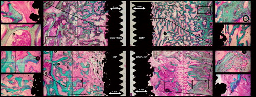
The study clearly indicates that there is a therapeutic window for both substances, which has clinical relevance. The consequences of missing this can be detrimental to implant fixation.

Study II (Table 5)

Hypothesis: When Colloss is added to allograft bone, early fixation of grafted implants is improved.

Table 5.  Change relative to control. “0”: no change. “+”: improvement. “−”: deterioration. The double signs “+ +” and “− −” indicate a group best or group worst

	Allograft treatment groups
	Control	Colloss 10 mg	Colloss 20 mg	Colloss 40 mg
Mechanical fixation	0	+	+ +	+
Implant osseointegration	0	+	+ +	+
Bone formation	0	+	+ +	+
Graft preservation	0	−	−	− −
Fibrous tissue reduction	0	+	+	+ +

Hypothesis disproved: No

Comments: Implant fixation was improved. The optimal dose seemed to be between 10 and 20 mg Colloss per cm³ packed allograft, which doubled the mechanical implant fixation. A dose‐dependent increase in increased allograft resorption was observed and was greatest by far in the high‐dose group (40 mg Colloss per cm³). A possible disadvantage of this was compensated by increased implant osseointegration and new bone formation.

Study III (Table 6)

Hypothesis: When Colloss E is added to a ceramic β‐TCP bone graft substitute (BGS), early fixation of grafted implants is improved and will be comparable to allografted implants.

Table 6.  Change relative to control. “0”: no change. “+”: improvement. “−”: deterioration

	Bone graft treatment groups
	Allograft	Allogr + Colloss E	BGS	BGS + Colloss E
Mechanical fixation	0	0		0
Implant osseointegration	0	0		+
Bone formation	0	0		0
Graft preservation	0	−		+/−
Fibrous tissue reduction	0	0		0

Hypothesis disproved: No

Comments: When Colloss E (20 mg per cm³ BGS) was added to β‐TCP granules, fixation was doubled and comparable to allograft. Implant osseointegration was better than both allografted groups. Colloss E increased resorption of both allograft and BGS, but had no effect on fixation of the allografted implants. Fibrous tissue was absent in the treated groups (Figures 31–33)

Figure 31. Study III; histology from two implants grafted with β‐TCP granules with Colloss E (left side) and without Colloss E (right side). Implants are not representative of group means and are from different animals.

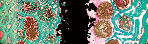
Figure 32. Study III; new bone formation on surface and in gap. Implant pairs interconnected +/− Colloss E (signal).

Figure 33. Study III; fibrous tissue on surface and in gap. Implant pairs interconnected +/− Colloss E (signal).

The study indicates that in the ongoing development of replacements for biological bone, substitution of osteogenic signalling may be just as important as the mechanical materials properties.

Perspective

The large animal experiment is an important step‐stone between in vitro studies and the human trial for developing new technologies in the area of implant fixation, bone healing and orthopaedics in general. Before inflicting potentially dangerous treatments on patients; even in strictly protocolled studies, as much information as possible should be obtained through experimental research. To understand tissue responses to treatments, animal experiments are invaluable.

In study I we failed to demonstrate any advantage in augmenting allograft with rhBMP‐2 and the bisphosphonate pamidronate. The metabolic effects of the substances were apparent: rhBMP‐2 stimulated new bone formation and prevented fibrous tissue encapsulation, but also caused increased allograft resorption. Pamidronate preserved the allograft, but also blocked new bone formation. This was also the case when rhBMP‐2 and pamidronate were combined, however the rhBMP‐2 seemed to also prevent fibrous tissue formation in this group despite its state of bone metabolic lock‐down. The metabolic effects where in other words abundant, resulting in a net negative influence on implant fixation which was likely related to the applied doses.

Manipulating a carefully regulated metabolic system which is still not fully understood is a delicate matter, and the study demonstrated that there is most likely a relatively narrow therapeutic window for a beneficial effect. This may be a future challenge because controlling the dose of topically delivered pharmaceuticals can be difficult. The evident effects of the substances on a tissue level lead us to believe, that pharmacological manipulation of bone metabolism at the site of traumatic bone healing has a large potential for future applications. However, there is still not sufficient evidence to recommend the use of anabolic or anti‐catabolic agents for bone graft and load‐bearing applications outside the context of strictly protocolled studies.

Study I did confirm that HA‐coated implants surrounded by bone graft are better osseointegrated and have better mechanical fixation then non‐coated implants.

In study II we demonstrated how allograft added lyophilised bovine bone matrix proteins prevented fibrous tissue formation, stimulated new bone formation and increased mechanical implant fixation. Higher doses gave increased allograft resorption, but at a level at which the net effect was still beneficial for implant fixation. An optimal dose seemed to lie around 10–20 mg of the Colloss device per cm³ allograft. We think that two of the advantages of devices derived from processed biological bone may be the occurrence of a range of agents contributing to bone formation as well as a possible delayed release of the active substances from the collagen I complexes in which they are presumed to be embedded.

This native origin may very well also be the disadvantage of Colloss and similar devices. It is difficult to determine the metabolically active content of the device, and at what dose it is applied. The device is a xenograft, and may trigger a foreign‐body response that may manifest differently in different patients. There may be large batch‐dependent differences in osteogenic capacity, and the costs of the product are relatively high, although not in comparison to recombinant BMPs.

In study III we applied the best dose found in study II of the equine equivalent, Colloss E, and used it as an osteogenic signal in a ceramic bone graft substitute packed around the implants. This improved osseointegration of the implant as well as the β‐TCP granules, and implant fixation was brought to a level comparable to the allografted implants. Resorption of the β‐TCP granules as well as the allograft was increased when Colloss E was applied, but Colloss E did not have a net negative influence on the mechanical implant fixation. In contrast to study II, Colloss E did not augment the fixation of the allografted implants. In the ongoing development of replacements for biological bone, we believe that substitution of osteogenic signalling may be just as important as substituting the mechanical properties of bone.

All three studies indicated that the increased new bone formation associated with the use of osteogenic growth factors was also associated with increased bone resorption. It seems that a bone anabolic stimulus is also to some extent also a catabolic stimulus. A future challenge will be to balance the net metabolic outcome, as was attempted in study I.