Gauge models of musical forces

Abstract

Metaphors involving motion and forces are a source of inspiration for understanding tonal music and tonal harmonies since ancient times. Starting with the rise of quantum cognition, the modern interactional conception of forces as developed in gauge theory has recently entered the field of theoretical musicology. We develop a gauge model of tonal attraction based on SU(2) symmetry. This model comprises two earlier attempts, the phase model grounded on U(1) gauge symmetry, and the spatial deformation model derived from SO(2) gauge symmetry. In the neutral, force-free case both submodels agree and generate the same predictions as a simple qubit approach. However, there are several differences in the force-driven case. It is claimed that the deformation model gives a proper description of static tonal attraction. The full model combines the deformation model with the phase model through SU(2) gauge symmetry and unifies static and dynamic tonal attraction.

1. Introduction

The phenomenon of tonal attraction has fascinated researchers of music psychology, both empirically and theoretically (Krumhansl and Cuddy 2010). There is a distinction between two types of tonal attraction, called static and dynamic attraction (Parncutt 2011). Static tonal attraction refers to how well a probe tone of a given pitch fits with a given tonal center. Dynamic tonal attraction, by contrast, refers to the level of harmonic resolution a listener feels when hearing a probe tone following a certain chord.

In a nowadays renowned study, Krumhansl and Kessler (1982) investigated the static type of tonal attraction. In this experiment, listeners were asked to rate how well each note of the chromatic octave fitted with a preceding context, which consisted of short musical sequences in major or minor keys. The results of this experiment clearly show a kind of hierarchy: the tonic pitch received the highest rating, followed by the pitches completing the tonic triad (third and fifth), then followed by the remaining scale degrees, and finally followed by the chromatic, non-scale tones. This finding plays an essential role in the later work of Lerdahl (e.g., Lerdahl 2001, 2015). It clearly counts as one of the main pillars of the structural approach in music theory. A related approach of the static type is due to Bharucha (1996).

The dynamic type of attraction was equally investigated by Krumhansl (1990, 1995), and many other researchers (e.g., Woolhouse 2009). Both types of tonal attraction have not only initiated an enormous number of empirical studies but also challenged a series of different models based on static and dynamic forces (see the subsequent section). Most of these models are close in inspiration to Larson (2012) in that they either explicitly or implicitly refer metaphorically to “musical forces” and build phenomenological models on this basis. These models aim at describing correlations instead of causal mechanisms which underlie tonal attraction.

The application of physical metaphors is quite common in theories of music. The basic assumption seems to be that our experience of musical motion is in terms of our experience of physical motion and their underlying forces. For example, Schönberg speaks about different forces when he explains the direction of musical movements in cadences where the tonic attracts the dominant (Schönberg [1911] 1978, 58). In addition, Larson and VanHandel (2005) proposed three musical forces that generate melodic completions. These forces are called gravity, inertia, and magnetism, respectively.

Musical gravity is the tendency (attributed by a listener) of a note (heard as ‘above a stable platform’) to descend (to that platform) […]. Musical magnetism is the tendency (attributed by a listener) of an unstable note to move to the closest stable pitch, a tendency that grows stronger as we get closer to that goal. […] Musical inertia is the tendency (attributed by a listener) of a pattern of motion to continue in the same fashion, where the meaning of ‘same’ depends on how that pattern is represented in musical memory. (Larson and vanHandel 2005, 122)

These forces should be regarded as conceptual metaphors in the sense of Lakoff and Johnson (1980). They structure our musical cognition in analogy with falling, inert, and attracting physical bodies. Physical forces are represented in our naïve common sense physics or folk physics. Analogously, musical forces cause musical dynamics in the naïve sense, that the impact of gravity yields to either ascending or descending melodic lines, depending on the position of a gravitation center. Magnetism should be larger, the closer a currently played tone is to a neighboring force center. And inertia refers to the observation that an already ascending or descending melody will remain ascending or descending in the sequel. Henceforth we refer to these models as to the metaphoric view of musical forces.

Yet, in modern physics, forces are closely related to symmetry and symmetry breaking. According to a famous theorem of Emmy Noether any (continuous) symmetry is accompanied with a conservation law (Neuenschwander 2017). Conservation of momentum, e.g., is related to the homogeneity of space: if it is not possible to highlight a distinguished point in space, then momentum does not change in the course of time. By contrast, the presence of a force center as a distinguished point breaks the homogeneity of space and momentum evolves according to Newton's second law: the particle is either attracted or repelled by the force center, resulting in positive or negative acceleration, respectively.

In contrast to Larson’s (2012) metaphorical usage of musical forces, Mazzola (1990, 2002) provides a quite different analogy between music theory and modern (non-folk) physics. Mazzola was probably the first who saw the close analogy between physics and music in connection with the existence of symmetries. In music, especially for the domain of modulation:

As force of transformation acts the instrument of modulation. The localization of “particles” is realized by means of the cadence of modulation. This kind of description is not unfamiliar to musicology: Schönberg, Uhde, and many others speak in a vague sense about forces between musical structures in order to explain musical changes in a comprehensible way. (Mazzola 1990, 200; our translation)

In order to codify Schönberg's ([1911] 1978) modulation theory, Mazzola (1990) invented the “modulation quantum” as a set of chords mediating musical transposition from one key into another key as a symmetry operation through exchange during cadences. Although we do not consider the domain of modulation in the present study, Mazzola's insights are of highest importance for our work. His theory sees the whole conception of “musical force” as directly rooted in the basic symmetry principles of tonal music. To distinguish the phenomenological (and metaphoric) idea of forces from the idea based on fundamental symmetries and physical interaction, we will call the latter view the structural realistic view (in short: realistic view). The idea is that the force conception plays a causal role in the theory. It is associated with a set of structural attributes that are necessary for the identity and function of physical and extra-physical forces within an interactional, symmetry-based theory of tonal music.

In the realistic view, forces are related to symmetry breakings. However, in modern quantum field theory, they obey a much deeper kind of symmetry, called local gauge symmetry. There, matter is described by a wave function (governed by a Schrödinger, Pauli or Dirac equation) and forces result from the coupling of the wave function with interaction fields. Locally gauging these interactions by the calibration of measurement devices is compensated by an unobservable phase shift of the matter's wave function. Therefore, it is always possible to make forces locally vanishing by means of a local gauge transformation. A decent example for such a gauge symmetry is provided by Einstein's general relativity theory where gravity vanishes in a free-falling reference system which is described by rulers and clocks whose calibration depends on space and time. In quantum field theory, matter wave functions and interaction fields are quantized, resulting into the exchange of virtual interaction particles that mediate the exertion of forces as local gauge transformations.

The present paper is concerned with the realistic view, which explains the existence of musical forces in terms of gauge transformations.¹ We suggest a universal model with SU(2) local gauge symmetry acting on two-dimensional complex spinor fields. This symmetry comprises two subgroups: first, U(1), the abelian group of local phase transformations in quantum theory. We call the corresponding model the phase model. And second, SO(2), the group of vector rotations in a two-dimensional (real) Hilbert space, which is related to the spatial deformation model of beim Graben and Blutner (2019). The combined model makes full use of the group SU(2).

We aim to demonstrate empirically that the spatial deformation model gives a proper description of static tonal attraction (tonal hierarchies as described in generative music theory, e.g. Lehrdahl 1988). In contrast, the phase model alone does not give much empirical support. However, in tandem with the deformation model it gives a fair description of dynamic attraction data, as investigated by Woolhouse (2009). The primary intent of this article is to present the novel idea of how to apply gauge theory in cognitive music theory. A detailed verification of the offered theory is outside of the scope of the present work.

The structure of the paper is as follows. The subsequent Section 2 explains basic experimental findings and their modeling by the metaphoric conception of musical forces. Section 3 presents the realistic view in terms of quantum cognition models. Section 4 explains the general idea of the structural realistic view and develops our gauge theory, which is subsequently applied to music cognition. Both static and dynamic attraction phenomena are discussed. Further, we explain how the hierarchic model of tonal attraction (Lerdahl 1988, 2001) can be remodeled within gauge theory. Section 5, finally, draws some general conclusions and raises issues for future research.

2. Metaphoric accounts to tonal attraction

Based on the experiments on static and dynamic tonal attraction, several authors proposed computational models that metaphorically refer more or less explicitly to notions of “musical forces.” Here, we briefly discuss two of the most influential models of those accounts, namely Lerdahl's hierarchical model of static attraction (Lerdahl 1988, 2001) and Larson's regression model of dynamic attraction (Larson 2012). Other important approaches are the interval cycle model of Woolhouse (2009) and Gaussian Markov chains (Temperley 2007).

In the following, we make use of the notion of a tonal pitch system. Such a system consists of a number of pitches which are sounds with a certain fundamental frequency. In this paper, we assume octave-equivalence resulting in twelve pitch classes, also called tones. Further, we assume a tuning system based on equal temperament, i.e. a tuning system in which the fundamental frequencies between adjacent notes have the same ratio.

The following numeric notation is used for defining the twelve tones of the system (“scale degree” j, with j running from 0 to 11), in ascending order Table 1:

Table 1. Pitch classes as chromatic scale degrees.

interval j	0	1	2	3	4	5	6	7	8	9	10	11	12
tone	C	D♭	D	E♭	E	F	G♭	G	A♭	A	B♭	B	C

2.1. Static attraction

Lerdahl (1988, 2001) and Lerdahl and Krumhansl (2007) have developed a model of tonal attraction based on a tonal hierarchy. Forerunners of this approach are Krumhansl (1979), Krumhansl and Kessler (1982) and Deutsch and Feroe (1981). A numerical representation of Lerdahl’s basic space for C-major is given in Table 2. It shows the twelve tones at their levels in the tonal hierarchy. In all, five levels are considered:

• A: octave space (defined by the root tone, C in the present case)

• B: open fifth space

• C: triadic space

• D: diatonic space (including all diatonic pitches of C-major in the present case)

• E: chromatic space (including all twelve pitch classes).

Table 2. The tonal pitch space as given in Lerdahl (1988).

A: octave

C

B: fifth

G

C: triadic

C

E

G

D: diatonic

C

D

E

F

G

A

B

E: chromatic

C

D♭

D

E♭

E

F

G♭

G

A♭

A

B♭

B

Anchoring strength s

4

0

1

0

2

1

0

3

0

1

0

1

Note: Pitch classes as chromatic scale degrees.

Table 2 also shows the tonal attraction or anchoring strength s(j) for pitch class j around the chroma circle. This measure simply counts the number of degrees that are commonly shared across levels A to D (omitting level E that is common for all tones).

Temperley (2008) proposed the following formula to calculate the attraction probability: (1) $p\left(j\right)=\frac{s\left(j\right)}{{\sum }_{j}s\left(j\right)}.$(1) The predictions of the hierarchical model are in excellent agreement with the experimental data in the case of major keys. In case of minor keys (based on the natural or harmonic minor scale), however, there are significant deviations (Blutner 2017; beim Graben and Blutner 2019). Regarding the function of the tonic hierarchy in tonal music, we refer to the insights of Philip Ball, which crucially address the tonal dynamics:

Although it is normally applied only to Western music, the word ‘tonal’ is appropriate for any music that recognizes a hierarchy that privileges notes to different degrees. That's true of the music of most cultures. In Indian music, the Sa note of a that scale functions as a tonic. It's not really known whether the modes of ancient Greece were really scales with a tonic centre, but it seems likely that each mode had at least a ‘special’ note the mese, that, by occurring most often in melodies, functioned perceptually as a tonic. This differentiation of notes is a cognitive crutch: it helps us interpret and remember a tune. The notes higher in a hierarchy offer landmarks that anchor the melody, so that we don't just hear it as a string of so many equivalent notes. Music theorists say that notes higher in this hierarchy are more stable, by which they mean that they seem less likely to move off somewhere else. Because it is the most stable of all, the tonic is where melodies come to rest. (Ball 2010, 95)

The probe tone techniques used in the experiments by Krumhansl and Kessler (1982) and others ask listeners directly to judge how well a single probe tone or chord fits an established context, and the relevant data collected by this technique represent the static tonal attraction.

2.2. Dynamic attraction

The finding that some tones are more stable than others invites some speculation about the dynamics of attraction. When considering sequences of pitches, “a melody is then like a stream of water that seeks the low ground” (Ball 2010, 95). The dynamic forces stipulated by Ball (2010) are forces that are directed towards the chromatic­ally closest tones that are higher in the static attraction hierarchy than the trigger. For the present purposes, it is enough to understand that dynamic attraction phenomena cannot be understood without their static counterparts. The models of Lerdahl (1996) and Lerdahl and Krumhansl (2007) realize this idea in an indirect way by requiring static attraction as one constituent of their dynamic attraction algorithm. In Section 4, we will review ‘realistic’ models that create a more direct connection.

Following Bharucha (1984), it is important to distinguish between “event hierarchies” and “tonal hierarchies” – the former reflecting melodic tension (dynamic attraction) and the latter reflecting harmonic tension (static attraction).² The dynamic type of attraction was investigated by Krumhansl (1990, 1995), Lerdahl and Krumhansl (2007), Lake (1987), Bharucha (1996), Lerdahl (1996), Larson (2004), Larson (2012), and in a study by Woolhouse (2009).

An interesting type of dynamic attraction data was collected in a probe-tone experiment based on the resolution of different chords (Woolhouse 2009). This experiment limits analysis to only the first new element after the presentation of the context chord. In the original experiments, five different context chords are considered: major triad {C, E, G}, minor triad {C, E♭, G}, dominant seventh {C, E, G, B♭}, French sixth {C, E, G♭, B♭}, or half-diminished seventh {C, E♭, G♭, B♭}. Probe tones are all twelve tones of the chromatic scale. The subjects had to decide (on a 7-point Likert scale) “the level of attraction and/or resolution they felt from the chord to the probe tone: seven for a high level of attraction, one for a low level of attraction” (Woolhouse 2009). In Section 4, we will come back to these data to evaluate our dynamic attraction model.

3. Realistic accounts to tonal attraction

What we call the realistic view in this article is due to ideas borrowed from theoretical physics. According to Penrose (2004, 289), all physical interactions are governed by “gauge connections” which crucially depend on exact symmetries. We assume these gauge connections as the fundamental principle of our realistic view of tonal forces. From the perspective of quantum physics, the idea of gauge symmetry has been applied by pioneers such as Schrödinger, Klein, Fock, and others (for an overview, see Jackson and Okun 2001, see also Supplement I for an intuitive introduction and for an outline of the standard example of electrodynamics).

Symmetries are mathematically formalized by group theory (e.g. Alexandroff 2012). For applying basic ideas of group theory to music (Balzano 1980; Mazzola 2002; Mazzola, Mannone, and Pang 2016), it is essential that there are certain operations that allow the transformation of tones into other tones. For instance, one can increase the tones by a certain number of steps 0, 1, 2, … ,11. Such operations are called transpositions. The 1-step transposition transforms C into D♭, D♭ into D, and so on.

Operations can be concatenated. For example, one can combine the transposition of a 2-step increase (a major second) with a 3-step transposition (a minor third), resulting in a 5-step transposition (a perfect fourth). We denote these operations likewise with the numbers 0, 1, 2, … , 11. Normally, the context makes clear what the numbers denote: a pitch class or the transposition operation, increasing tones by a number of elementary steps. It is obvious that the concatenation of transpositions can be described by addition modulo 12: i = j + k mod 12; e.g. 2 + 3 mod 12 = 5, 7 + 6 mod 12 = 1.

In the case of music based on twelve tones, we have to consider the set of group elements 0, 1, 2, … ,11, and the group operation is j ∘ k = j + k mod 12. The neutral element is the element denoted by 0, (0 + j) mod 12 = (j + 0) mod 12 = j. For the inverse element we have j⁻¹= (12−j) mod 12. The group consisting of the 12 tones is the cyclic group G = ${\mathbb{Z}}_{12}$. Note that a group G is called cyclic if there exists a single element g ∈ G such that every element in G can be generated as a composition k g mod 12. The element g is hence called a generator of the group.

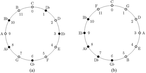
In the numerical representation of the cyclic group ${\mathbb{Z}}_{12}$ there are four generators represented by the numbers 1,11,7, and 5. Hence, 1 (one minor second upward) and 11 (one minor second downward) generate the sequence of semitones. In addition, the elements 5 and 7 enumerate the group elements in successive fourths or fifths, respectively, thereby generating the circle of fifths. Figure 1 gives a visual representation of the group ${\mathbb{Z}}_{12}$ using the two basically different generators 1 or 11 (Figure 1(a)), and 7 or 5 (Figure 1(b)). The group G = ${\mathbb{Z}}_{12}$ describes the fundamental transposition symmetry of Western tonal music in equal temperament (Balzano 1980).

Figure 1. Group structure ${\mathbb{Z}}_{12}$ of Western music in equal temperament for C major key. (a) Chroma circle of C major scale as generated by minor seconds. (b) Circle of fifths as generated by perfect fifths (clockwise) and perfect fourths (counterclockwise). Open bullets indicate scale (diatonic) tones; closed bullets denote non-scale (chromatic) tones.

3.1. Qubit model

Next, we construct a simple geometric representation of the symmetry group ${\mathbb{Z}}_{12}$ of Western tonal music. Such a representation is given by matrices as studied in linear algebra. More specifically, the group ${\mathbb{Z}}_{12}$ is isomorphic to a particular group of real rotation matrices for vectors in a two-dimensional real vector space.

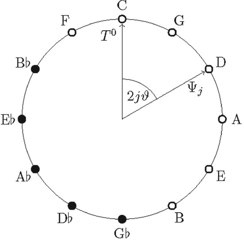
For instance, we consider the vector (2) $T^0=\left(\begin{array}{c}1\\ 0\end{array}\right)$(2) indicating the tonic j = 0 in Figure 1. Henceforth, we refer to such a particular vector as to the tonic vector in our exposition.

From the tonic vector $T^0$, all tones of the circle of fifths can be generated through 12 successive rotations by means of an elementary rotation matrix, (3) $R=\left(\begin{array}{cc}\text{cos }\vartheta & -\text{sin }\vartheta \\ \text{sin }\vartheta & \text{cos }\vartheta \end{array}\right),$(3) with basic rotation angle ϑ = π/12. Iterating these rotations j times (j ∈${\mathbb{Z}}_{12}$), we obtain all tones: (4) ${\mathrm{\Psi }}_j={\mathit{R}}^j\cdot T^0=\left(\begin{array}{c}\text{cos }j\vartheta \\ \text{sin }j\vartheta \end{array}\right).$(4) Particularly, we have ${\mathrm{\Psi }}_0={\mathit{R}}^0\cdot T^0=T^0$ and ${\mathrm{\Psi }}_6={\mathit{R}}^6\cdot T^0=\left(\begin{array}{c}\text{cos}\left(\frac{\pi }{2}\right)\\ \text{sin}\left(\frac{\pi }{2}\right)\end{array}\right)=\left(\begin{array}{c}0\\ 1\end{array}\right)$. Thus, the circle of fifths is represented in a two-dimensional quantum bit (“qubit”) Hilbert space spanned by the tonic vector Ψ₀= $T^0$ and its orthogonal complement Ψ₆, representing the tritone G♭ in Figure 2 (Blutner 2017).³

Figure 2. Qubit model in two-dimensional Hilbert space based on the circle of fifths.

In the qubit model, tonal attraction is evaluated through projections. A tone $j\in {\mathbb{Z}}_{12}$ at the circle of fifths is represented through its state vector Ψ_j. Then, its attraction value exerted by the tonic is given as the squared modulus of the scalar product, (5) $p\left(j\right)=|{\mathrm{\Psi }}_j\cdot T^0{|}^2=\text{co}{\text{s}}^{2}j\vartheta =\text{co}{\text{s}}^2\frac{j\pi }{12}.$(5) The probabilities calculated in (5) describe the attraction between a probe tone j and the tonic context $T^0$ (single tone) alone. In order to account for complex chord contexts as well, Woolhouse (2009), Woolhouse and Cross (2010), and Blutner (2017) suggested to average the attraction profiles of individual pairs of tones over all possible pairings between probe tone and context tones.

For N context tones $k_i\in {\mathbb{Z}}_{12}$ in a chord $C=\{k_i\in {\mathbb{Z}}_{12}|i=1,\dots ,N\}$ with individual weight factors $\rho \left(k_i\right)$, we have a discrete convolution, (6) $p_C\left(j\right)=\sum _{i=1}^N\rho \left(k_i\right)\cdot p\left(j-k_i\right),$(6) with kernel $p\left(j\right)$ given in (5).

3.2. Scalar wave model

So far, we have considered tones as isolated entities, which are represented by vectors in a two-dimensional Hilbert space. From the point of view of information processing in the cochlea and in the auditory cortex this is not a very plausible assumption. Already the phenomenon of frequency separation across the basilar membrane suggest a field model of tonal perception, which is closely related to the “place theory” of acoustic information processing based on Helmholtz (1863) and his followers. The basic idea is the existence of a (one-dimensional) manifold and the assumption that the different tones correspond to topologically different parts of this configuration space. Specific­ally, we choose the unit circle, parameterized by a single continuous variable x ∈ [0, 2π], as tonal configuration space and embed the discrete circle of fifths by real numbers x = jπ/6 ($j\in {\mathbb{Z}}_{12}$, with C(0) $\cong$ C’(12) one octave higher).

The free quantum model suggested by beim Graben and Blutner (2017, 2019) comprises a tonic wave function, (7) $\psi \left(x\right)=\frac{1}{\sqrt{\pi }}\cos \frac{x}{2}$(7) such that the quantum probability density (8) $p\left(x\right)=|\psi \left(x\right){|}^2=\psi (x{)}^{\ast }\psi \left(x\right)$(8) for a given interval x yields the tonal attraction value (9) $p\left(x\right)=\frac{1}{\pi }\text{co}{\text{s}}^2\frac{x}{2}$(9) 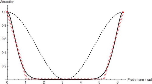is in agreement with the qubit model of Section 3.1 for x = jπ/6.⁴ The dashed line of Figure 3 shows the attraction profile corresponding to (9).

Figure 3. Quantum models of tonal attraction. It shows the qubit kernel (dashed), the static deformation kernel (solid), and the kernel function resulting from the classical hierarchic model (dotted). Note that the endpoints correspond to the tonic tone (0 $\cong$ 12). Due to the chosen normalization, the maximum of the profiles is 1 in all cases.

The formalism of quantum mechanical wave functions allows the application of the operator calculus from functional analysis in order to assess the contributions of musical forces in a realistic account. To this end, we first derive a field equation from (7(7) $\psi \left(x\right)=\frac{1}{\sqrt{\pi }}\cos \frac{x}{2}$(7) ) that can be interpreted as a Schrödinger equation of a “force-free particle” (Busemeyer and Bruza 2012) moving along the circle of fifths. In a second step, we introduce a spatial deformation of the phases in (7(7) $\psi \left(x\right)=\frac{1}{\sqrt{\pi }}\cos \frac{x}{2}$(7) ). This deformation leads to another field equation involving several differential operators which assume a straightforward interpretation as musical forces. Finally, these forces are related to gauge fields of a continuous symmetry. Differentiating (7(7) $\psi \left(x\right)=\frac{1}{\sqrt{\pi }}\cos \frac{x}{2}$(7) ) twice yields an ordinary differential equation of second order: (10) $-{\text{ψ}}^{\mathrm{\prime }\mathrm{\prime }}\left(x\right)=\frac{1}{4}\text{ψ}\left(x\right)$(10) which can be interpreted as an eigenvalue equation $H\text{ψ}\left(x\right)=E\text{ψ}\left(x\right)$ with Hamilton operator $H=(-{\mathrm{\partial }}^2/\mathrm{\partial }{x}^2)$ and eigenvalue $E=1/4$. Hence, equation (10(10) $-{\text{ψ}}^{\mathrm{\prime }\mathrm{\prime }}\left(x\right)=\frac{1}{4}\text{ψ}\left(x\right)$(10) ) turns out to be the quantum mechanical stationary Schrödinger equation for the motion of a “free particle” with kinetic energy E = 1/4 along the circle of fifths. The operator (11) $H=-\frac{{\mathrm{\partial }}^2}{\mathrm{\partial }{x}^2}\left(=T\right)$(11) must therefore realistically be interpreted as the operator of inertia force or kinetic energy.

In order to improve the concordance between model and the tonal attraction data of Krumhansl and Kessler (1982) and Woolhouse (2009), beim Graben and Blutner (2017, 2019) introduced a suitable deformation of the distances along the circle of fifths by the ansatz (12) $\text{ψ}\left(x\right)=\frac{1}{\sqrt{\pi }}\cos \gamma \left(x\right)$(12) for the stationary wave function where $\gamma \left(x\right)$ is an arbitrary spatial deformation function. The wave function (12) yields the following probability density. (13) $p\left(x\right)=|\text{ψ}\left(x\right){|}^2=\frac{1}{\pi }\text{co}{\text{s}}^2\gamma \left(x\right)$(13)

Differentiating (12(12) $\text{ψ}\left(x\right)=\frac{1}{\sqrt{\pi }}\cos \gamma \left(x\right)$(12) ) twice again and eliminating trigonometric terms, we then obtain the differential equation, (14) $-{\text{ψ}}^{\mathrm{\prime }\mathrm{\prime }}\left(x\right)+\frac{{\gamma }^{{}^{\mathrm{\prime }\mathrm{\prime }}}\left(x\right)}{{\gamma }^{\mathrm{\prime }}\left(x\right)}{\text{ψ}}^{\mathrm{\prime }}\left(x\right)-\gamma {}^{\mathrm{\prime }}(x{)}^2\text{ψ}\left(x\right)=0\text{.}$(14) In order to get the standard form of the stationary Schrödinger equation, we decompose the Hamiltonian into three parts. (15) $H=T+M+U\text{ with }T=-\frac{{\mathrm{\partial }}^2}{\mathrm{\partial }{x}^2},M=\frac{{\gamma }^{\mathrm{\prime }\mathrm{\prime }}\left(x\right)}{{\gamma }^{\mathrm{\prime }}\left(x\right)}\frac{\mathrm{\partial }}{\mathrm{\partial }x},U=E-\gamma {}^{\mathrm{\prime }}(x{)}^2$(15) Then equation (14(14) $-{\text{ψ}}^{\mathrm{\prime }\mathrm{\prime }}\left(x\right)+\frac{{\gamma }^{{}^{\mathrm{\prime }\mathrm{\prime }}}\left(x\right)}{{\gamma }^{\mathrm{\prime }}\left(x\right)}{\text{ψ}}^{\mathrm{\prime }}\left(x\right)-\gamma {}^{\mathrm{\prime }}(x{)}^2\text{ψ}\left(x\right)=0\text{.}$(14) ) becomes again an eigenvalue problem: $H\text{ψ}\left(x\right)=E\text{ψ}\left(x\right)$. In equation (15(15) $H=T+M+U\text{ with }T=-\frac{{\mathrm{\partial }}^2}{\mathrm{\partial }{x}^2},M=\frac{{\gamma }^{\mathrm{\prime }\mathrm{\prime }}\left(x\right)}{{\gamma }^{\mathrm{\prime }}\left(x\right)}\frac{\mathrm{\partial }}{\mathrm{\partial }x},U=E-\gamma {}^{\mathrm{\prime }}(x{)}^2$(15) ), the first term T is the operator of inertia as for the free model. The second term M could realistically be interpreted as magnetic interaction energy. Supplement I gives the physicist’s motivation for connecting it with the magnetic force. Finally, the last term in the Hamiltonian (15(15) $H=T+M+U\text{ with }T=-\frac{{\mathrm{\partial }}^2}{\mathrm{\partial }{x}^2},M=\frac{{\gamma }^{\mathrm{\prime }\mathrm{\prime }}\left(x\right)}{{\gamma }^{\mathrm{\prime }}\left(x\right)}\frac{\mathrm{\partial }}{\mathrm{\partial }x},U=E-\gamma {}^{\mathrm{\prime }}(x{)}^2$(15) ), which is simply a scalar multiplication operator, receives its usual interpretation as potential energy $U=E+V\left(x\right)$, which might be seen as the potential of the electrostatic force – with the static potential $V\left(x\right)=-\gamma {}^{\mathrm{\prime }}(x{)}^2$. Note that the expected total energy density is $\text{ψ}(x{)}^{\ast }\cdot H\text{ψ}\left(x\right)=E\cdot p\left(x\right).$ Hence, we can identify it with the static attraction profile.⁵

Next, one can ask for suitable choices of the deformation function $\gamma \left(x\right)$. beim Graben and Blutner (2019) argue that plausible interpolation conditions imply that $\gamma \left(0\right)=0$ and $\gamma \left(\pi \right)=\pi /2$. A consequence of this choice is that the tonic (at 0) should not be deformed while the tritone (at $\pi$) receives maximal deformation. A simple polynomial of fourth order that satisfies the two interpolation conditions is as follows. (16) $\gamma \left(x\right)=\frac{\pi }{2}-\frac{{\left(x-\pi \right)}^4}{2{\pi }^3}$(16) With this deformation function, beim Graben and Blutner (2019) found excellent agreement with the static attraction data of Krumhansl and Kessler (1982). Figure 3 also presents the comparison between our two quantum models and the kernel function reconstructed from Lerdahl’s (1988) classical hierarchical model (dotted line).

There is a simple, intuitive argument for the choice of a non-linear deformation function such as in equation (16(16) $\gamma \left(x\right)=\frac{\pi }{2}-\frac{{\left(x-\pi \right)}^4}{2{\pi }^3}$(16) ). As Figure 3 reveals, the kernel function for static tonal attraction (solid line) assigns the maximum value to the target tone, in our case the tonic C. The two neighbours on the circle of fifths (i.e. G and F) receive an attraction value that is about half of it. The attraction values of all other tones is very low such that they are negligible. Hence, constructing the attraction profiles for a certain context given by a triad, e.g. CEG, we obtain an approximate reconstruction of the hierarchic model. The three tones of the triad CEG receive a very high value, C and G a bit larger than E because of the convolution operation. Next, the neighbours of the triadic tones (C: G, F; G: D, C; E: B, A) are all diatonic tones and get an attraction of about 50%. Hence, we can account for all levels of the hierarchic model shown in Table 2 besides the octave level (resulting in four different degrees of attraction).

3.3. Spinor wave model

Qubits, as introduced by Blutner (2017) into mathematical musicology, live in a two-dimensional complex vector space. Therefore, in the next step we combine the qubit model from Section 3.1 with the scalar wave function models of Section 3.2 for obtaining a two-dimensional spinor field theory. This structural complication has several advantages: (i) it allows including the deformation idea in a novel, more systematic way; (ii) it provides a closer connection between static and dynamic attraction; (iii) it gives an explanation for certain asymmetries that underlie the distinction between major and minor modes of tonality.⁶ We come back to the first two issues in Sect. 4; the last issue is outlined in the final part of supplement I.

Replacing the scalar tonal attraction equation (13(13) $p\left(x\right)=|\text{ψ}\left(x\right){|}^2=\frac{1}{\pi }\text{co}{\text{s}}^2\gamma \left(x\right)$(13) ) by an equation for a spinor field, (17) $\mathrm{\Psi }\left(x\right)=\left(\begin{array}{c}{\text{ψ}}_1\left(x\right)\\ {\text{ψ}}_2\left(x\right)\end{array}\right),$(17) we obtain the so-called Pauli equation (Pauli 1927) in its most general form, (18) $-{\mathrm{\Psi }}^{\mathrm{\prime }\mathrm{\prime }}\left(\text{x}\right)+\mathit{M}\left(x\right)\cdot {\mathrm{\Psi }}^{\mathrm{\prime }}\left(\text{x}\right)+\mathit{V}\left(x\right)\cdot \mathrm{\Psi }\left(x\right)=0,$(18) with coupling matrices $\mathit{M}\left(x\right)$ and $\mathit{V}\left(x\right)$ for magnetic interaction and (electro-)static potential, respectively (see Supplement I). The Pauli equation is a not a scalar wave equation such as the Schrödinger equation but rather a wave equation governing a two-dimensional vector field, called the spinor field, where every spinor component essentially obeys a separate Schrödinger equation with additional coupling terms between spinor components.⁷

For the force-free case, the Pauli equation (18(18) $-{\mathrm{\Psi }}^{\mathrm{\prime }\mathrm{\prime }}\left(\text{x}\right)+\mathit{M}\left(x\right)\cdot {\mathrm{\Psi }}^{\mathrm{\prime }}\left(\text{x}\right)+\mathit{V}\left(x\right)\cdot \mathrm{\Psi }\left(x\right)=0,$(18) ) decouples into a pair of free Schrödinger equations with $\mathit{M}\left(x\right)=0$ and a diagonal matrix $\mathit{V}\left(x\right)=v\left(x\right)1$, v(x) = −1/4. Then equation (18(18) $-{\mathrm{\Psi }}^{\mathrm{\prime }\mathrm{\prime }}\left(\text{x}\right)+\mathit{M}\left(x\right)\cdot {\mathrm{\Psi }}^{\mathrm{\prime }}\left(\text{x}\right)+\mathit{V}\left(x\right)\cdot \mathrm{\Psi }\left(x\right)=0,$(18) ) has the fundamental solution (19) $\mathrm{\Psi }\left(x\right)=\frac{1}{\sqrt{\pi }}\left(\begin{array}{c}\cos \frac{x}{2}\\ \sin \frac{x}{2}\end{array}\right).$(19) The probability that a probe tone is attracted by the tonic with constant spinor $T^0$ of equation (2(2) $T^0=\left(\begin{array}{c}1\\ 0\end{array}\right)$(2) ) is then obtained by the projection (20) $p\left(x\right)=|\mathrm{\Psi }\left(x\right)\cdot T^0{|}^2.$(20)

For the free-particle solutions (19) we obtain (21) $p\left(x\right)=|\mathrm{\Psi }\left(x\right)\cdot T^0{|}^2=\frac{1}{\pi }{\cos }^2\frac{x}{2},$(21) i.e. the same attraction ratings as for the qubit and the free scalar wave function models. In the next section, we will see the advantages of the spinor approach in connection with the introduction of gauge forces.

4. Realistic models based on gauge symmetry

For the force-free case, the three quantum models discussed above, namely the qubit model, the scalar Schrödinger wave function model and the spinor Pauli wave function model yield identical predictions for static and dynamic tonal attraction. Using different kinds of spatial deformations, such as the polynomial one in (16), beim Graben and Blutner (2019) were able to improve the empirical agreement between the scalar wave model and data from static and dynamic tonal attraction experiments. However, in both settings different deformation functions had to be employed. For static attraction, the deformation (16) rendered the kernel reconstructed from the hierarchical model of Lerdahl (1988) – see Figure 3 (dotted line). Yet, for dynamic attraction another deformation had to be constructed by hand from Woolhouse’s interval cycle model (Woolhouse 2009).

In this section, we demonstrate how a realistic approach to musical forces in terms of musical gauge symmetry can provide a parsimonious and unifying picture of static and dynamic attraction. Additionally, several other advantages will become obvious. We start with the hypothesis that all musical forces are gauge forces and that any gauge force is founded in a symmetry group and a gauge field (for technical details, see Supplement I). Gauge symmetry is essentially related to the distinction between overt and covert physical quantities. The value of a wave function is covert as it cannot be directly observed in physical measurement. Measurable are only probabilities and expectation values. Both elements are based on scalar products – see equation (20(20) $p\left(x\right)=|\mathrm{\Psi }\left(x\right)\cdot T^0{|}^2.$(20) ). Hence, they must be invariant under unitary transformations. The standard example of a unitary transformation is a shift of the wave function’s phases. In case of spinors, another unitary transformation is the rotation of the spinor (see Section 3.1).

4.1. SU(2) gauge symmetry: three gauge models of tonal attraction

For investigating the general case of the spinor wave model, we consider here the non-abelian group SU(2) of special unitary 2×2 matrices U with unit determinant. This group is generated by the Pauli matrices (22), (22) ${\sigma }_1=\left(\begin{array}{cc}0& 1\\ 1& 0\end{array}\right),{\sigma }_2=\left(\begin{array}{cc}0& -i\\ i& 0\end{array}\right),{\sigma }_3=\left(\begin{array}{cc}1& 0\\ 0& -1\end{array}\right).$(22) It is possible to construct the unitary matrix by the generating expression (23) $\mathit{U}=e^{-\frac{i}{2}\sum _{j=1}^3{\delta }_j\left(x\right)\cdot {\sigma }_j}\text{ ,}$(23)

for an arbitrary local gauge transformation with real phase functions δ₁(x), δ₂(x), and δ₃(x). Evaluating the matrix exponential in (23) entails the general SU(2) transformation matrix (24) $\mathit{U}\left(\vartheta ,\varphi ,\tau \right)=\left(\begin{array}{cc}\text{cos }\vartheta e^{-i\varphi }& -\text{sin }\vartheta e^{i\tau }\\ \sin \vartheta e^{-i\tau }& \text{cos }\vartheta e^{i\varphi }\end{array}\right)$(24) where we distinguish ϑ = δ₁(x),τ = δ₂(x), $\varphi$ = δ₃(x).

In the force-free case, we have used the spinor $\mathrm{\Psi }\left(x\right)$ of equation (19(19) $\mathrm{\Psi }\left(x\right)=\frac{1}{\sqrt{\pi }}\left(\begin{array}{c}\cos \frac{x}{2}\\ \sin \frac{x}{2}\end{array}\right).$(19) ). Gauge forces are realized by applying the unitary transformation U to the spinor: (25) $\mathrm{\Psi }\left(x\right)\to \tilde{\mathrm{\Psi }}\left(x\right)=\mathit{U}\left(\vartheta ,\varphi ,\tau \right)\mathrm{\Psi }\left(x\right).$(25)

In Supplement II, some technical details are explained. In this section, we consider the calculation of probability densities only, which is similar to equation (20(20) $p\left(x\right)=|\mathrm{\Psi }\left(x\right)\cdot T^0{|}^2.$(20) ). Instead of projecting the spinor $\mathrm{\Psi }\left(x\right)$ to the tonic spinor, we now project the gauge-transformed spinor $\tilde{\mathrm{\Psi }}\left(x\right)$ and calculate the square of its length. For simplicity, we assume that the phase functions $\varphi \left(x\right)$ and $\tau \left(x\right)$ are identical.

In order to get an optimal agreement of our model with the experimental evidence on both static and dynamic attraction, we exploit some additional freedom by suitably rotating the tonic spinor introduced in (2). Using (26) $T^3=\frac{1}{\sqrt{2}}\left(\begin{array}{c}1\\ 1\end{array}\right)$(26) instead of (2), we apply the gauge transformation $\mathit{U}\left(\vartheta ,\varphi ,\varphi \right)$ to the force-free solution (19). Then, a simple calculation gives the following probability density: (27) $\tilde{p}\left(x\right)=|\tilde{\mathrm{\Psi }}\left(x\right)\cdot T^3{|}^2=\frac{1}{2\pi }\left(1+\cos x\sin 2\vartheta \left(x\right)+\sin x\cos 2\vartheta \left(x\right)\cos 2\varphi \left(x\right)\right).$(27)

In order to compensate for the rotation of the tonic, we transpose the kernel function as follows. (28) $p\left(x\right)=\tilde{p}\left(x+\frac{\pi }{2}\right)$(28) In the density function p(x), the tonic corresponds to x = 0 and the tritone to x=π. The definition of the matrix (24) allows for several special cases. We consider three cases, for which we obtain three different kernel functions.

4.1.1. Deformation SO(2) model

First, we consider the setting τ=ϕ=0 which provides the SO(2) gauge group, described in Section 3.1, equation (3(3) $R=\left(\begin{array}{cc}\text{cos }\vartheta & -\text{sin }\vartheta \\ \text{sin }\vartheta & \text{cos }\vartheta \end{array}\right),$(3) ), therefore U(ϑ,0,0) = R. We demonstrate now that this gauge symmetry leads to the deformation model describing static tonal attraction for the particular gauge (16). From equation (27(27) $\tilde{p}\left(x\right)=|\tilde{\mathrm{\Psi }}\left(x\right)\cdot T^3{|}^2=\frac{1}{2\pi }\left(1+\cos x\sin 2\vartheta \left(x\right)+\sin x\cos 2\vartheta \left(x\right)\cos 2\varphi \left(x\right)\right).$(27) ) we regain the SO(2) deformation model. (29) ${\tilde{p}}_D\left(x\right)=\frac{1}{2\pi }\left(1+\cos x\sin 2\vartheta \left(x\right)+\sin x\cos 2\vartheta \left(x\right)\right).$(29) Performing the substitution (28) yields (30) $\begin{array}{rl}{p}_D\left(x\right)=\tilde{p}\left(x+\frac{\pi }{2}\right)& =\frac{1}{2\pi }\left[1+\cos \left(x+\frac{\pi }{2}\right)\sin 2\vartheta \left(x+\frac{\pi }{2}\right)+\sin \left(x+\frac{\pi }{2}\right)\cos 2\vartheta \left(x+\frac{\pi }{2}\right)\right]\\ & =\frac{1}{2\pi }\left[1+\sin \left(x+\frac{\pi }{2}+2\vartheta \left(x+\frac{\pi }{2}\right)\right)\right]\\ & =\frac{1}{2\pi }\left[1+\cos \left(x+2\vartheta \left(x+\frac{\pi }{2}\right)\right)\right]=\frac{1}{\pi }{\cos }^2\left(\frac{x}{2}+\vartheta \left(x+\frac{\pi }{2}\right)\right).\end{array}$(30)

When we compare the result of (30(30) $\begin{array}{rl}{p}_D\left(x\right)=\tilde{p}\left(x+\frac{\pi }{2}\right)& =\frac{1}{2\pi }\left[1+\cos \left(x+\frac{\pi }{2}\right)\sin 2\vartheta \left(x+\frac{\pi }{2}\right)+\sin \left(x+\frac{\pi }{2}\right)\cos 2\vartheta \left(x+\frac{\pi }{2}\right)\right]\\ & =\frac{1}{2\pi }\left[1+\sin \left(x+\frac{\pi }{2}+2\vartheta \left(x+\frac{\pi }{2}\right)\right)\right]\\ & =\frac{1}{2\pi }\left[1+\cos \left(x+2\vartheta \left(x+\frac{\pi }{2}\right)\right)\right]=\frac{1}{\pi }{\cos }^2\left(\frac{x}{2}+\vartheta \left(x+\frac{\pi }{2}\right)\right).\end{array}$(30) ) with equation (13(13) $p\left(x\right)=|\text{ψ}\left(x\right){|}^2=\frac{1}{\pi }\text{co}{\text{s}}^2\gamma \left(x\right)$(13) ) (scalar wave model) we see that both accounts agree assuming the following gauge function $\vartheta \left(x\right)$. (31) $\vartheta \left(x+\frac{\pi }{2}\right)=\gamma \left(x\right)-\frac{x}{2}\text{or}\vartheta \left(x\right)=\gamma \left(x-\frac{\pi }{2}\right)-\frac{x}{2}+\frac{\pi }{4}$(31) Hereby, the deformation function $\gamma$ is given as equation (16(16) $\gamma \left(x\right)=\frac{\pi }{2}-\frac{{\left(x-\pi \right)}^4}{2{\pi }^3}$(16) ).

4.1.2. Phase U(1) model

Second, we set ϑ = 0, $\tau =\varphi$, such that (32) $\mathit{U}\left(0,\varphi ,\varphi \right)=\left(\begin{array}{cc}{e}^{-i\varphi }& 0\\ 0& e^{i\varphi }\end{array}\right)=e^{-i\varphi {\sigma }_3}.$(32)

These matrices belong to an abelian subgroup of SU(2) that is isomorphic to the U(1) phase model. As kernel, we obtain (33) ${\tilde{p}}_P\left(x\right)=\frac{1}{2\pi }(1+\sin x\cos 2\varphi (x\left)\right).$(33)

Again, we apply the transformation (28). This results in the superposition of two phase-shifted kernels: (34) $p_P\left(x\right)=\frac{1}{2\pi }\left[{\cos }^2\left(\frac{\text{x}}{2}+\varphi \left(x+\frac{\pi }{2}\right)\right)+{\cos }^2\left(\frac{\text{x}}{2}-\varphi \left(x+\frac{\pi }{2}\right)\right)\right].$(34) In the next subsection, we give a graphical representation of this function for a particular phase gauge.

It should be noted that it is important to take $T^3$ (see equation (26(26) $T^3=\frac{1}{\sqrt{2}}\left(\begin{array}{c}1\\ 1\end{array}\right)$(26) )) to get this form of the kernel function. In case we take the tonic $T^0$, which is the spinor $\left(\begin{array}{c}1\\ 0\end{array}\right)$, we obtain a rather trivial result, namely the free particle solution of equation (21(21) $p\left(x\right)=|\mathrm{\Psi }\left(x\right)\cdot T^0{|}^2=\frac{1}{\pi }{\cos }^2\frac{x}{2},$(21) ) – a solution that does not depend on the form of the phase gauge $\varphi \left(x\right)$.

4.1.3. Combined SU(2) model

Finally, we consider a combination of phase model and deformation model. Again, we assume that both phase functions are identical, i.e. $\tau =\varphi$. The corresponding transformation matrix is (35) $\mathit{U}\left(\vartheta ,\varphi ,\varphi \right)=\left(\begin{array}{cc}\text{cos }\vartheta e^{-i\varphi }& -\text{sin }\vartheta e^{i\varphi }\\ \sin \vartheta e^{-i\varphi }& \text{cos }\vartheta e^{i\varphi }\end{array}\right)$(35) where the SO(2) gauge function ϑ(x) refers to the static deformation model, while the U(1) gauge function $\varphi$(x) will be deployed as a phase model of dynamic attraction in the sequel. The calculated kernel function is defined by equation (27(27) $\tilde{p}\left(x\right)=|\tilde{\mathrm{\Psi }}\left(x\right)\cdot T^3{|}^2=\frac{1}{2\pi }\left(1+\cos x\sin 2\vartheta \left(x\right)+\sin x\cos 2\vartheta \left(x\right)\cos 2\varphi \left(x\right)\right).$(27) ), repeated here: (36) ${\tilde{p}}_{D+P}\left(x\right)=\frac{1}{2\pi }\left(1+\cos x\sin 2\vartheta \left(x\right)+\sin x\cos 2\vartheta \left(x\right)\cos 2\varphi \left(x\right)\right).$(36) The index $D+P$ refers to the combination of Deformation and Phase model. After applying the transformation (27), the variable x is running from 0 to $2\pi .$ The gauge function $\vartheta \left(x\right)$ is given by (31). For the phase gauge we assume (37) $\varphi \left(x\right)=x.$(37)

Hence, the first derivation of this gauge function is a constant. Obviously, this is the simplest case of a gauge field with a constant potential function.

Figure 4 shows the kernel functions of the three gauge models. Deformation and phase model are mirror-symmetric around the tritone.⁸ Interestingly, the combination of both models is not mirror-symmetric. As a matter of fact, the combination is not simply the sum of the two terms given in (29) and (33). Rather, it contains interference terms that violate the mirror-symmetry.

Figure 4. Kernel function for (a) deformation gauge, (b) phase gauge, (c) the equal combination of both gauge fields.

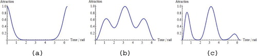
The three models are based on (a) the deformation field alone, (b) the phase field alone, and (c) a combination of both fields. Interestingly, the combination shows a breaking of the mirror symmetry resulting from the interference of the two involved gauge fields.

4.2. Dynamic attraction

As outlined in Section 2.2, several authors have proposed a connection between static and dynamic attraction. The present SU(2) gauge model equally establishes a close connection between static and dynamic attraction. Hence, the combination of the deformation model and the phase model (even in its simplest form with a constant phase field) supplies a novel description of the dynamic attraction data of Woolhouse (2009). We already noted that the combined model violates the mirror symmetry (relative to the position of the tritone). In other words, it breaks the mirror symmetry of the dynamic kernel function. Since the deformation model itself satisfies mirror symmetry, we recognize that the combination with the phase gauge field is responsible for the broken mirror symmetry.

We have calculated the correlation functions of different models with the dynamic attraction data of Woolhouse (2009). The predictions of the combined model are shown in Table 3. We considered two variants of the combined model: (i) deformation and phase model are coupled equally (assuming $\varphi \left(x\right)=x$), (ii) the phase model is weakened (assuming $\varphi \left(x\right)=.85x$).⁹ Further, we show the correlations for the ICP model of Woolhouse (2009).¹⁰

Table 3. Correlation of the ICP model and the combined gauge model with dynamic attraction data (Woolhouse 2009).

Correlation with dynamic attraction data	ICP model	Combined model $\left(\phi \right(x)=x\mathrm{a}\mathrm{n}\mathrm{d}\phi (x)=.85x)$
C-major	.69	.11	.55
C-minor	.78	.29	.7
dominant seventh	.75	.37	.76
French sixth	.79	.9	.86
half-dimin. seventh	.89	.6	.78
Correlations with ICP		0.4	0.6

Note: For the combined gauge model we consider two variants. In the first case, deformation and phase model are coupled equally. In the second case, the phase model is coupled with 85% only. The dynamic attraction data concern (a) major triad CEG, (b) minor triad CE♭G, (c) dominant seventh CEGB♭, (d) French sixth CEG♭B♭, and half-diminished seventh CE♭G♭B♭. For all models, including the ICP model, the correlation with dynamic attraction data has been shown.

The ICP model exhibits a similar quality for describing the dynamic attraction data as the combined model (second variant). However, the ICP model is not able to describe the static attraction data.¹¹

5. Discussion

In this article, we have contrasted the metaphoric and the realistic conceptions of musical forces. Both approaches provide interesting perspectives to study static and dynamic tonal attraction profiles, including their structure, use, and acquisition. The metaphoric conception is taken from mainstream cognitive psychology initiated by work of Lakoff (1987) and Lakoff and Johnson (1980, 1999). The realistic conception of musical forces is a new development within the evolving field of quantum cognition and regards musical forces as gauge forces. The present study discussed both approaches.

We have started with the metaphoric conception. Notably, a conceptual metaphor refers to the understanding of one conceptual field in terms of another one. Famous examples illustrating the idea are “life is a journey” or “time is money.” According to this concept, musical forces are constructs in analogy to our understanding of physical forces in folk physics. Various authors have proposed different forces, which are assumed to be important for music perception. Linear regression analysis has been applied in order to find the total effect of musical forces. Unfortunately, the fits achieved with empirical data are not really convincing. A sound grounding of forces does not seem feasible in this way (see Supplement III).

In contrast, the realistic conception of musical forces constructs tonal attraction as gauge forces, which can be derived from fundamental symmetries of the underlying theory and a gauge field. In the present case, we model tones by vectors of a two-dimensional spinor Hilbert space. Hence, the basic symmetry is the group of special unitary transformations SU(2) and their subgroups.

In a sense, the proposed realistic conception is a fresh implementation of Kepler’s 400-year- old vision of Harmonices Mundi (Kepler 1619) — the vision unifying physics and musicology. Recognizing the failing of Kepler’s ideas — mainly for reasons that concern certain astronomical facts, unknown yet 400 years ago — the present approach is based on a totally different scenery centred around the insights of modern quantum cognition (Busemeyer and Bruza 2012).

We have identified the symmetry group SU(2) as the fundamental group that directs the gauge theoretic approach.¹² This symmetry can be described by matrix transformations acting on a two-dimensional spinor space. This transformation group is determined by three generators. In general, they relate to three independent gauge fields. Here, we have identified the deformation model of static tonal attraction (beim Graben and Blutner 2019) with one of the three gauge fields of the SU(2) symmetry, on the one hand. On the other hand, a combination of deformation and phase model accounts for dynamic tonal attraction.

Concerning the results of the gauge theoretic modeling attitude, we stress three aspects that we regard as the central pillars of the present study. First, the idea of discrete convolution — an operation describing the modification of a kernel function by a distribution of several contextual elements (for instance, the tones of a single chord). Second, in contrast to a related study (beim Graben and Blutner 2019) where two different deformation functions have been constructed for independently describing static and dynamic attraction, the present approach unifies both kinds of musical forces in a single theoretical framework. The basic idea of connecting static and dynamic attraction goes back to several authors. Our unifying gauge model establishes a close connection between static and dynamic attraction in a novel way. The gauge field of the deformation model explains static attraction. By adding the gauge field of the phase model, we are able to explain dynamic attraction data. Third, the combined model — in its simplest form with a linear gauge field — breaks the mirror symmetry of the dynamic kernel function. This gauge field has further consequences. Even with a very weak coupling of 3%, the mirror symmetry of the static attraction kernel is already broken. This may provide an unusual explanation for the fundamental asymmetry between major and minor modes. It goes without stressing the point, of course, that capital efforts are needed for providing a proper verification of the present theory. The primary intent of the present article has been the presentation of a novel theory, while its verification will be postponed to subsequent research in mathematical musicology.

In Section 2 we have introduced the hierarchical model of tonal attraction and in Section 4 we have explained how it can be reconstructed within the quantum framework. There are two important facts that can be described by the hierarchical model: First, for both major and minor profiles, scale tones have higher values of tonal attraction than non-scale tones. Second, all tones of the tonic triad have higher values than other tones of the scale.

In the hierarchical model, these two important empirical facts are directly stipulated in a rather ad hoc way by assuming a “diatonic space” (level D) which includes all scale notes and by assuming a higher order “triadic space” (level C) that includes the tones of the triadic space. Importantly, the present quantum model starts from very general assumptions about symmetries and has only to stipulate the tonic triad in order to explain all the mentioned facts (Blutner 2017). Further, as has been pointed out in Section 4.2, the present model but not the hierarchical model is able to explain the close connection between static and dynamic attraction.

Finally, yet importantly, we mention an unresolved issue, which could be an essential point for future research. It concerns the highly debated issue of innateness. Already Leonard Bernstein has vehemently disputed this issue by expressing and stressing that musical apperception is not possible without an innate cognitive background. At the end of his Norton lectures (Bernstein 1976), he formulates his deep belief in the tonal system through the following magical phrases.

I believe that from that Earth emerges a musical poetry which is by the nature of its sources tonal.

I believe that these sources cause to exist a phonology of music, which evolves from the universal known as the harmonic series,

And that there is an equally universal syntax, which can be codified and structured in terms of symmetry and repetition. (Bernstein 1976)

In the present context, this innate background is mainly constituted by fundamental symmetries of tonal music. They give rise to the proposed tonal kernel function and operations such as discrete convolution that are not acquired during learning.¹³

The phenomenon of tonal attraction and the phenomenon of graded consonance/dissonance are closely related according to several authors (e.g., Large 2010; Parncutt 1989, 2011; Krumhansl 1990). However, for building the distinction between consonance and dissonance, learned parameters seem to play a much more important role than usually assumed (McDermott et. al., 2016). Other authors still see potential for biological explanations (Bowling and Purves 2015; Bowling et al. 2017). Hence, the empirical debate is still open and novel theoretical ideas that illuminate how biology and culture interact to shape how we experience tonal music are of continued interest.

Supplemental online material

Supplemental online material for this article can be accessed at doi:10.1080/17459737.2020.1716404.

Acknowledgements

We are indebted to Stefan Blutner, Maria Mannone, and Günther Wirsching for discussion, and to Guerino Mazzola, Stuart Hammeroff and Jerome Busemeyer for their encouragement. Two anonymous reviewers and the editors of the Journal of Mathematics and Music are warmly acknowledged for their helpful and stimulating comments.

Disclosure statement

No potential conflict of interest was reported by the authors.

Notes

1 This suggests a causal role of musical forces and their effects on musical perception and cognition. Obviously, we can find the relevant symmetries both in physics and musicology – supposing the basic traits of applying the mechanism of quantum mechanics for the area of cognitive psychology are accepted (Busemeyer and Bruza 2012).

2 Note that Lerdahl’s (1988) model does not provide a corresponding quantification of melodic, as opposed to harmonic, tension.

3 In order to avoid confusion: In the circle of Figure 2, the angle runs from 0 to 2$\pi$ such that tonic and tritone are on opposite sites of the circle. The ‘real’ angles of the Hilbert-space vectors must be half of this such that tonic and tritone become orthogonal to each other. Thus, in the ‘real’ rotation matrix (3) we have to divide the angles by the number 2 in order to get the angles in the rotation matrix.

4 Of course, this choice of discrete values for the twelve tones corresponds straightforwardly with the choice of equal temperament system of tuning. In a microtonal context or other systems of tuning, different systems of discrete values are expected (Gómez-Téllez, Lluis-Puebla, and Montiel 2017). In principle, such values can be represented by the present mechanism. However, authors such as Burns (1999) argue that the basic scale structure even in Indian and other non-Western cultures is likewise due to the 12-tone chromatic structure. So-called microtones (shrutis) are normally slight variations of certain intervals. There is evidence that in real musical practice these microtonal variations are not played as discrete intervals but relate to a variability in intonation such as a slow vibrato. The present quantum model is also supported by experimental findings of Krumhansl and Shepard (1979) who augmented a tonal attraction experiment by additionally using quartertones besides the chromatic scale as probes. They reported that tonal attraction ratings at quartertones interpolate the ratings measured at scale tones. Thus, tonal attraction at semi- or quartertones can be seen as a discrete sampling of the underlying continuous wave function.

5 The terms “inertia,” “magnetism,” or “electrostatic force” of the emergent terms in the Schrödinger equation (14(14) $-{\text{ψ}}^{\mathrm{\prime }\mathrm{\prime }}\left(x\right)+\frac{{\gamma }^{{}^{\mathrm{\prime }\mathrm{\prime }}}\left(x\right)}{{\gamma }^{\mathrm{\prime }}\left(x\right)}{\text{ψ}}^{\mathrm{\prime }}\left(x\right)-\gamma {}^{\mathrm{\prime }}(x{)}^2\text{ψ}\left(x\right)=0\text{.}$(14) ) are not at all related to the metaphorical intuitions in musicology, inspired by interpreting these concepts in terms of folk physics (Larson and VanHandel 2005; Larson 2012). In the present, realistic interpretation only the sum of these terms has a musical interpretation (as static attraction). This contrasts with the metaphoric models, were the single terms of the regression analysis are interpreted musically. Earlier research (beim Graben and Blutner 2017) has explicitly calculated the three terms “inertia,” “magnetism,” and “electrostatic force.” However, these authors found that only the sum of these terms has a proper musical interpretation and not the shape of the single functions.

6 See Stolzenburg (2015) for a recent review of many relevant empirical and theoretical issues.

7 We should stress again, that in both cases – Schrödinger equation and Pauli equation – we consider the stationary case only. Of course, one can argue that their time-dependent counterparts are required in order to analyse the temporal development of the wave functions and, thus, the development of melodies and chordal sequences. In the classical setting (using Bayesian probabilities and Markov chains) such time-dependencies in fact have been considered – for instance in the work of Temperley (2008). However, a quantum approach for time-dependent phenomena goes far beyond the scope of the present article.

8 Of course, it is an easy exercise to calculate the energy densities for kinetic energy, magnetism, and electrostatics separately for the two gauges and their combination. Unfortunately, we do not see any empirical ideas yet that could profit from such a detailed analysis.

9 The weakening of the coupling lifts the right peak in Figure 4(c) and shrinks the center one.

10 Assuming twelve-tone equal temperament, the interval-cycle proximity (ICP) of a tonal interval is defined as the smallest positive number such that the product with the interval length (i.e. the number of half tone steps spanned by the interval) is a multiple of 12 (maximal interval length). For example, the ICP for the tritone is 2 and the ICP for the fifth is 12.

11 In a recent article, Quinn (2010) reviewed Woolhouse's ICP hypothesis. There, he suggested another hypothesis better fitting the empirical data, called “Melody Harmonic Proximity” (MHP). However, Quinn did not realize that the ICP hypothesis is based on a principled, systematic approach, whereas the MHP model only provides a purely phenomenological description. Hence, the ICP is not fitted on empirical data, while the MHP is. This is achieved by explicitly constructing its kernel function from phenomenal properties of the data. According to Woolhouse and Cross (2011) this procedure provides a “self-fulfilling prophecy.” In our opinion, the methodological position of Woolhouse and his colleagues is largely appreciated. Yet we believe it might be too rigid. In our own approach, we have at least one empirical parameter that cannot be theoretically derived (the strength of coupling between deformation and phase model). Table 3 illustrates that a suitable choice of the parameter can yield predictions similar to that of the ICP hypothesis. In order to avoid misunderstandings: the present paper does not aim to give a detailed empirical verification of the present model. Hence, we did not provide a serious parameter fitting, and the important work of empirical verification is left for future enterprises.

12 See Supplement II for outlining the role of SU(2) in modern particle physics.

13 Concerning the innateness issue, there are two extreme positions. On the one hand, some authors propose innate perceptual principles – such as the ICP principle (Woolhouse and Cross 2010, 2011). On the other hand, traditional Bayesian approaches downplay the role of innateness and assume a straightforward learning mechanism (e.g., Temperley 2007, 2008). The position taken by the present authors lies somewhere in between the extremes: assuming an innate background based on certain symmetry principles and stipulating a learning mechanism to fix the available free parameters.

References

- Alexandroff, Paul. 2012. An Introduction to the Theory of Groups. New York: Dover.
- Ball, Philip. 2010. The Music Instinct: How Music Works and why we Can't do Without it. London: Bodley Head.
- Balzano, Gerald J. 1980. “The Group-Theoretic Description of 12-Fold and Microtonal Pitch Systems.” Computer Music Journal 4 (4): 66–84. doi: 10.2307/3679467
- beim Graben, Peter, and Reinhard Blutner. 2017. “Toward a Gauge Theory of Musical Forces.” In Quantum Interaction. 10th International Conference (QI 2016), LNCS 10106, edited by J. A. de Barros, B. Coecke, and Emanuel Pothos, 99–111. Berlin: Springer.
- beim Graben, Peter, and Reinhard Blutner. 2019. “Quantum Approaches to Music Cognition.” Journal of Mathematical Psychology 91: 38–50. doi: 10.1016/j.jmp.2019.03.002
- Bernstein, Leonard. 1976. The unanswered question: Six talks at Harvard. Princeton: Harvard University Press.
- Bharucha, Jamshed J. 1984. “Anchoring Effects in Music: The Resolution of Dissonance.” Cognitive Psychology 16: 485–518. doi: 10.1016/0010-0285(84)90018-5
- Bharucha, Jamshed J. 1996. “Melodic Anchoring.” Music Perception 13 (3): 383–400. doi: 10.2307/40286176
- Blutner, Reinhard. 2017. “Modelling Tonal Attraction: Tonal Hierarchies, Interval Cycles, and Quantum Probabilities.” Soft Computing 21 (6): 1401–1419. doi: 10.1007/s00500-015-1801-7
- Bowling, Daniel L., Marisa Hoeschele, Kamraan Z. Gill, and W. Tecumseh Fitch. 2017. “The Nature and Nurture of Musical Consonance.” Music Perception 35 (1): 118–121. doi: 10.1525/mp.2017.35.1.118
- Bowling, Daniel L, and Dale Purves. 2015. “A Biological Rationale for Musical Consonance.” Proceedings of the National Academy of Sciences 112 (36): 11155–11160. doi: 10.1073/pnas.1505768112
- Burns, Edward M. 1999. “Intervals, Scales, and Tuning.” In The Psychology of Music, edited by Diana Deutsch, 215–264. New York: Academic Press.
- Busemeyer, Jerome R., and Peter D. Bruza. 2012. Quantum Cognition and Decision. Cambridge: Cambridge University Press.
- Deutsch, Diana, and J. Feroe. 1981. “The Internal Representation of Pitch Sequences in Tonal Music.” Psychological Review 88: 503–522. doi: 10.1037/0033-295X.88.6.503
- Gómez-Téllez, J. D., E. Lluis-Puebla, and M. Montiel. 2017. “A Symmetric Quantum Theory of Modulation in Z 20.” In Mathematics and Computation in Music. MCM 2017. Lecture Notes in Computer Science, vol 10527, edited by O. Agustín-Aquino, E. Lluis-Puebla, and M. Montiel, 50–62. Cham: Springer.
- Helmholtz, Hermann von. 1863. Die Lehre von den Tonempfindungen als Physiologische Grundlage für die Theorie der Musik. Braunschweig: Friedrich Vieweg und Sohn.
- Jackson, John David, and Lev Borisovich Okun. 2001. “Historical Roots of Gauge Invariance.” Reviews of Modern Physics 73 (3): 663–694. doi: 10.1103/RevModPhys.73.663
- Krumhansl, Carol L. 1979. “The Psychological Representation of Musical Pitch in a Tonal Context.” Cognitive Psychology 11: 346–374. doi: 10.1016/0010-0285(79)90016-1
- Krumhansl, Carol L. 1990. Cognitive Foundations of Musical Pitch. New York: Oxford University Press.
- Krumhansl, Carol L. 1995. “Music Psychology and Music Theory: Problems and Prospects.” Music Theory Spectrum 17: 53–80. doi: 10.2307/745764
- Krumhansl, Carol L., and Lola L. Cuddy. 2010. “A Theory of Tonal Hierarchies in Music.” In Music Perception, edited by Mari Riess Jones, Richard R. Fay, and Arthur N. Popper. 51–87. New York: Springer.
- Krumhansl, Carol L., and Roger N. Shepard. 1979. “Quantification of the Hierarchy of Tonal Functions Within a Diatonic Context.” Journal of Experimental Psychology: Human Perception and Performance 5 (4): 579–594.
- Krumhansl, Carol L., and Edward J. Kessler. 1982. “Tracing the Dynamic Changes in Perceived Tonal Organization in a Spatial Representation of Musical Keys.” Psychological Review of General Psychology 89: 334–368. doi: 10.1037/0033-295X.89.4.334
- Lake, William E. 1987. “Melodic perception and cognition: The influence of tonality.” Unpublished doctoral dissertation. University of Michigan.
- Lakoff, George. 1987. Women, Fire, and Dangerous Things: What Categories Reveal About the Mind. Chicago: University of Chicago Press.
- Lakoff, George, and Mark Johnson. 1980. Metaphors We Live By. Chicago: University of Chicago Press.
- Lakoff, George, and Mark Johnson. 1999. Philosophy in the Flesh: The Embodied Mind and Its Challenge to Western Thought. New York: Basic Books.
- Large, Edward W. 2010. “A Dynamical Systems Approach to Musical Tonality.” In Nonlinear Dynamics in Human Behavior, edited by Raoul Huys and Viktor K. Jirsa, 193–211. Berlin: Springer.
- Larson, Steve. 2004. “Musical Forces and Melodic Expectations: Comparing Computer Models and Experimental Results.” Music Perception 21 (4): 457–498. doi: 10.1525/mp.2004.21.4.457
- Larson, Steve. 2012. Musical Forces: Motion, Metaphor, and Meaning in Music. Bloomington: Indiana University Press.
- Larson, Steve, and Leigh VanHandel. 2005. “Measuring Musical Forces.” Music Perception 23 (2): 119–136. doi: 10.1525/mp.2005.23.2.119
- Lerdahl, Fred. 1988. “Tonal Pitch Space.” Music Perception 5 (3): 315–350. doi: 10.2307/40285402
- Lerdahl, Fred. 1996. “Calculating Tonal Tension.” Music Perception 13 (3): 319–363. doi: 10.2307/40286174
- Lerdahl, Fred. 2001. Tonal Pitch Space. NewYork: Oxford University Press.
- Lerdahl, Fred. 2015. “Concepts and Representations of Musical Hierarchies.” Music Perception 33 (1): 83–95. doi: 10.1525/mp.2015.33.1.83
- Lerdahl, Fred, and Carol L. Krumhansl. 2007. “Modeling Tonal Tension.” Music Perception 24 (4): 329–366. doi: 10.1525/mp.2007.24.4.329
- Mazzola, Guerino. 1990. Geometrie der Töne. Basel: Birkhäuser.
- Mazzola, Guerino. 2002. The Topos of Music: Geometric Logic of Concepts, Theory, and Performance. Basel: Birkhauser.
- Mazzola, Guerino, Maria Mannone, and Y. Pang. 2016. Cool Math for Hot Music. New York: Springer International Publishing Switzerland.
- McDermott, Josh H., Alan Schultz, Eduardo Undurraga, and Ricardo Godoy. 2016. “Indifference to Dissonance in Native Amazonians Reveals Cultural Variation in Music Perception.” Nature 25: 21–25.
- Neuenschwander, Dwight E. 2017. Emmy Noether's Wonderful Theorem. Baltimore: Johns Hopkins University Press.
- Parncutt, Richard. 1989. Harmony: A Psychoacoustical Approach. Berlin: Springer.
- Parncutt, Richard. 2011. “The Tonic as Triad: Key Profiles as Pitch Salience Profiles of Tonic Triads.” Music Perception: An Interdisciplinary Journal 28 (4): 333–366. doi: 10.1525/mp.2011.28.4.333
- Pauli, Wolfgang. 1927. “Zur Quantenmechanik des Magnetischen Elektrons.” Zeitschrift für Physik 43 (9): 601–623. doi: 10.1007/BF01397326
- Penrose, Roger. 2004. The Road to Reality. London: Jonathan Cape.
- Quinn, Ian. 2010. “On Woolhouse's Interval-Cycle Proximity Hypothesis.” Music Theory Spectrum 32 (2): 172–179. doi: 10.1525/mts.2010.32.2.172
- Schönberg, Arnold. (1911) 1978. Harmonielehre. Wien Verlagsanstalt Paul Gerin (Translated by R. E. Carter as: Theory of Harmony. Berkeley: University of California Press, 1978).
- Stolzenburg, Frieder. 2015. “Harmony Perception by Periodicity Detection.” Journal of Mathematics and Music 9 (3): 215–238. doi: 10.1080/17459737.2015.1033024
- Temperley, David. 2007. Music and Probability. Cambridge: Mass.: MIT Press.
- Temperley, David. 2008. “A Probabilistic Model of Melody Perception.” Cognitive Science 32 (2): 418–444. doi: 10.1080/03640210701864089
- Woolhouse, Matthew. 2009. “Modelling Tonal Attraction Between Adjacent Musical Elements.” Journal of New Music Research 38 (4): 357–379. doi: 10.1080/09298210903180252
- Woolhouse, Matthew, and Ian Cross. 2010. “Using Interval Cycles to Model Krumhansl's Tonal Hierarchies.” Music Theory Spectrum 32 (1): 60–78. doi: 10.1525/mts.2010.32.1.60
- Woolhouse, Matthew, and Ian Cross. 2011. “To The Editor: A Response to Ian Quinn.” Music Theory Spectrum 33 (1): 99–105. doi: 10.1525/mts.2011.33.1.99