Use of Landsat and MODIS data to remotely estimate Russia’s sown area

Abstract

The intensity of crop management is one of the most important management decisions that affect soil carbon stocks in croplands. In this study, we use satellite data at two spatial resolutions (30 m Landsat and 500 m MODIS) and field observations to determine arable lands in a portion of the Russian grain belt. Once arable lands are established, we map cropping intensity between 2002 and 2009 to get a better understanding of the activity occurring on arable lands. Our arable land estimates compare favourably with the 2006 All-Russia Agricultural Census. We also compare three global data sets that quantify croplands against the census data. Finally, we show that our cropping intensity map compares very well to the available regional statistical data. We reveal that areas in the southern regions of Russia are successfully cropped during fewer years than more centrally located areas.

Keywords:

• cropland extent
• cropland intensity
• Russia
• phenology
• MODIS
• Landsat

1. Introduction

Widespread land abandonment was perhaps the most vivid side effect of the agricultural reform that occurred after the collapse of the Soviet Union (Ioffe, 2005; Ioffe, Nefedova, & Zaslavsky, 2004). We have demonstrated that for large agricultural areas, such as the spring grain regions in Kazakhstan, cropland abandonment can be detected even with coarse spatial resolution image time series (NOAA AVHRR, 8 km) (de Beurs & Henebry, 2004). In Kazakhstan, we found that abandonment had significant effects on land surface phenology: grasses and weedy forbs growing in former croplands tended to green-up before crops were typically planted (de Beurs & Henebry, 2004). Cropland abandonment patterns have been studied with satellite data in Eastern Europe (Hölzel, Haub, Ingelfinger, Otte, & Pilipenko, 2002; Kuemmerle, Hostert, Radeloff, Perzanowski, & Kruhlov, 2007; Kuemmerle, Radeloff, Perzanowski, & Hostert, 2006) as well as in Kazakhstan, Turkmenistan, Uzbekistan and Afghanistan (de Beurs & Henebry, 2004, 2005a, 2008b; Henebry, de Beurs, & Gitelson, 2005; Hölzel et al., 2002). Many of these studies compared cropland patterns before and after 1991, the year in which the Soviet Union broke up.

In general, agricultural intensification is used to refer to a number of different processes: (1) an increase in inputs such as fertilizers or water; (2) management practices, such as crop rotation, fallow and cropping intensity (Rounsevell et al., 2012). In this study, we are interested in management changes as measured by cropping intensity. The intensity of crop management, e.g. continuous cropping versus crop rotations with periods of bare fallow, is one of the most important management decisions that affect soil carbon stocks in croplands (Lasco et al., 2006). Various crop-rotation schemes are applied in global grain belts, some including four or more crops, while others include only one (e.g. wheat–fallow system often applied in Canada). The main purpose of fallow periods in crop rotations is to build up water storage in the soil profile for subsequent crops. A clean fallow period also helps to diminish weed infestations. Clean fallow refers to a period during which no crops are planted on the land and the soil is regularly tilled to eliminate weeds. Summer clean farming is still a regularly used practice in Russia and Central Asia and is thought to be one of the leading factors affecting the depletion of soil organic carbon in these regions (Lal, 2004). Russian farmers employ a variety of crop-rotation schemes. In the past, most farmers in the grain belt used a 7-year rotation, which typically included only 1 year of clean fallow and a variety of grain crops in the remaining 6 years ((Lindeman, 2003), and field interviews). Further south, in Northern Kazakhstan, a 4-year cycle was widely recommended with summer fallow once in 4 years (Suleimenov et al., 2005). There are signs that the crop rotations are changing, with some areas increasing the number of years of fallow and others planting cover crops instead of using a summer clean fallow period ((Lindeman, 2005; Suleimenov et al., 2005),author field visits). In addition, new (modern) investors, interested in re-cultivating previously abandoned areas in our study region, are re-evaluating their crop management decisions carefully (e.g. (Stanislav, Jonsson, Kust, & Zetterquist, 2010) and observed during author field visits). Besides being a management decision, the number of years a field is sown with crops and actually growing crops (which we define as cropping intensity) is also influenced by drought. Severe droughts often result in crop failure (Dronin & Bellinger, 2005). Between 1900 and 1990, droughts occurred approximately 36% of the time in the Central Volga Region (Dronin & Bellinger, 2005).

There are a large number of research papers discussing the use of remotely sensed data in the estimation of cropland area and crop types. Some of these papers combine Landsat data with coarser resolution imagery such as data from NOAA AVHRR (Rembold & Maselli, 2006) or MODIS (e.g. Fritz, Massart, Savin, Gallego, & Rembold, 2008; Lobell & Asner, 2004). While some only map croplands, others map different crop types as well (e.g. Fritz et al., 2008). When croplands are mapped it is typical to indicate arable lands without identifying cropping intensity, although in some instances fallow is mapped as a crop category (Fritz et al., 2008). The presence of crops on a field has an influence on not only CO₂ flux but also albedo, roughness, length and soil moisture (Lokupitiya et al., 2009). Over the past few years, a number of studies have focused on the mapping of tillage practices in the United States, with the goal of identifying no-till practices which are a growing management decision in North American croplands (Watts, Powell, Lawrence, & Hilker, 2011; Zheng, Campbell, & de Beurs, 2012).

While several studies have focused on ongoing abandonment in Russian croplands, few have focused on current cropping intensity and we are not aware of any map indicating cropping intensity in Russia. In this study, we will first use remotely sensed observations to map the available arable lands. Once the locations of arable lands are established, we will map cropping intensity between 2002 and 2009 to get a better understanding of the activity occurring on arable lands. We will utilize satellite data at two spatial resolutions (30 m Landsat and 500 m MODIS) and field observations to determine arable lands in the Russian grain belt (Figure 1). We will determine cropping intensity by using phenological metrics based on MODIS data. We validate the 30 m Landsat classifications based on field observations and fine scale satellite data available through Google Earth. We compare the final results for arable land estimates with the 2006 All-Russia Agricultural Census (Laykam, 2006) to get an idea as to how closely the remotely sensed data set corresponds to independently collected statistics. We also compare the results to an independently collected Google Earth data set containing 721 MODIS samples. We validate our cropping intensity map for 5 years in Samara oblasts which we visited and where we have regional statistical data on cropping intensity.

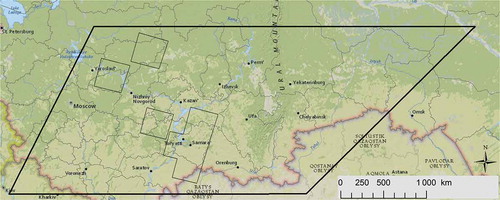
Figure 1. Overview figure with outlines of the two MODIS tiles (thick lines) and the Landsat images (thin line).

While we will create our own arable land data for our study region, we will also evaluate the three most recent global land cover classification products: the MODIS IGBP at 500 m resolution (Friedl et al., 2010), the Global Cropland Extent (Pittman, Hansen, Becker-Reshef, Potapov, & Justice, 2010) and the MERIS GlobCover 2009 data at 300 m (Bontemps et al., 2011). A thorough comparison between coarse resolution land cover maps based on GLC-2000, GlobCover and MODIS for Northern Eurasia was carried out by Pflugmacher et al. (2011). They found only a moderate to fair agreement between the global data sets in six test sites spread over Northern Eurasia (Pflugmacher et al., 2011). However, they did not specifically address differences in croplands. An extensive global evaluation for the MODIS IGBP land cover data set and the MERIS GlobCover data with respect to croplands was conducted by Fritz et al. (2011). In their report, they found that the overall spatial disagreement between these two data sets for the cropland classes is very high. It appears that the MODIS product is overestimating the croplands in the Russian grain belt compared to MERIS. The Global Cropland Extent data were previously evaluated against several other cropland data sets: Geographic distribution of global agricultural lands (Ramankutty, Evan, Monfreda, & Foley, 2008), MOD12Q1 (same product as used here) and the GLC-2000 (Pittman et al., 2010). Pittman et al. (2010) suggest that the agreement between the three land cover maps is not as certain in Russia as it is in other areas mainly because they compared the data against some heritage data sets from the early 1990s. They argue that these heritage data sets estimated croplands before the majority of the abandonment (estimated 30–40%) as a result of the collapse of the Soviet Union took place. Since they only provide a map inter-comparison, it is unclear which map provides a better crop estimate. In contrast with what we present here, Fritz et al. (2011) present a map inter-comparison without evaluating independent statistical observations. However, the Geo-wiki website, which forms the basis of the Fritz et al. (2011, 2012) articles, does provide a comparison between country wide statistics (Fritz et al., 2012). For Russia, the country wide statistics are based on FAO arable lands data from 2000 and 2005. There are no regional statistics included.

1.1. Agricultural and arable lands definitions

Several definitions are available for agricultural and arable lands. We use the definition from FAO which defines arable land as land under temporary crops, temporary meadows for mowing or for pasture, land under market or kitchen gardens and land temporarily laid fallow. Temporarily fallowed land is land set aside for one or several years before being cultivated again. Land abandoned as a result of shifting cultivation is excluded. Arable lands are distinguished from agricultural lands which also include permanent pastures. Permanent pastures are lands used for five or more years for herbaceous forage crops, either cultivated or growing wild. The definition for arable lands does not include lands that are potentially cultivable. Agricultural land refers to the land area that is arable, under permanent crops and under permanent pastures (http://data.worldbank.org/indicator/AG.LND.AGRI.ZS).

It is very hard to distinguish between fallow land and lands that are abandoned based on remote sensing data alone. In the field this is a difficult classification as well. While traveling around the Russian country side, we have seen several examples of fields that are considered arable land, but that are not currently in use. Some of these fields were set aside temporarily with the ultimate goal of using them again in the near future; some of these fields were used only once in a while to maintain them. We have also seen examples of fields that were previously abandoned and were currently in use and vice versa. We have learned that areas that were continuously cropped year after year were less likely to be abandoned in the future (Ioffe et al., 2004). For this article, we consider the final classification (e.g. not used or abandoned) as being less important. Instead, we want to know if a particular piece of land is successfully sown or not in a particular year. What we mean with this is whether or not the fields that were seeded in a particular spring resulted in a harvest. Unsuccessfully or not sown fields could be a result of management decisions (e.g. the farmer set the field aside in a particular year and did not sow it) or weather impacts (a severe drought may prevent a successful year).

2. Data

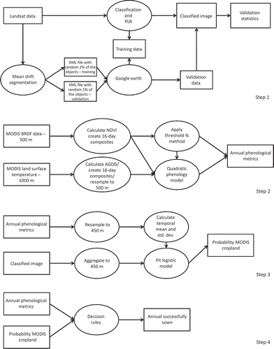
The data collected and the processing steps are summarized in Figure 2. The data and methods can be divided into four steps. The first step generates a classified Landsat image. The second step creates a set of annual phenological metrics based on MODIS time series data. The third step combines the classified Landsat map with the annual phenological metrics in a logistic regression model to generate a MODIS probability map for cropland. We validate this map against data from the 2006 All-Russia Agricultural Census carried out by the Russian Federation Federal State Statistics Service (Rosstat) (Laykam, 2006) and against 721 random samples checked with high-resolution Google Earth data. The final step, applies a set of decision rules to determine whether pixels that we identified as cropland between 2002 and 2009 were in fact cropped in a particular year. We validate these data against statistical yearbook data that we acquired when we visited Samara oblast in 2010.

Figure 2. Overview of the methodology in four steps.

2.1. Statistical data

In this study, we use the census data from the All-Russia Agricultural Census which was conducted in July 2006 and consisted of approximately 30 million questionnaires. The content and procedure of the census were developed based on recommendations from FAO and other international organizations. The full account of the agricultural census was released in 2008. In addition, we collected official statistical data and updated lower level district data collected previously (Ioffe, 2005; Pallot & Nefedova, 2007) during two field trips in May/June 2010 and October 2011. Most of the statistical data are available per rayon. For example, one such statistic is total area sown with crops. These data exist for crop type and farm type (household farms, registered private farms and large-scale commercial farms). The total area of successfully sown land is available for all rayons in Samara oblast only, which is the region we visited (Agriculture Samara, 2004, s.224, 2009, s.100–101). The data set includes this variable for the years 2004 through 2008.

We also visited typical settlements and enterprises in Samara and Kostroma oblast and Chuvash Republic. We interviewed rural administration heads, farm managers and the local population during our visit. We took field photographs and corresponding GPS coordinates, which were used during land cover classification.

2.2. Landsat data

We used Landsat data from seven different path/row combinations which were chosen to correspond to the areas which we visited. Our time series consisted of available Landsat 5 images for each tile between 2006 and 2011, except for one image in September 1998 in path 172, row 22. Each path/row was represented by images during the peak of the growing season and the spring or the fall, with a focus on the fall to enable the capturing of winter wheat growth (Table 1). All images were atmospherically corrected with the ENVI FLAASH routine. FLAASH is a first-principles atmospheric correction tool that corrects wavelengths in the visible region through near-infrared and shortwave infrared regions, and incorporates the MODTRAN4 radiation transfer code. After correction, all the available bands, except the thermal band, were stacked into one file per path/row.

Table 1. Overview of Landsat images

Samara Oblast				Chuvash Republic	Kostroma Oblast
169/22	169/23	169/24	170/23	172/22	176/20	174/19
14 JUL 2006	2 AUG 2007	2 AUG 2007	29 JUL 2009	15 SEP 1998	15 MAY 2007	2 AUG 2006
18 AUG 2007	18 AUG 2007	18 AUG 2007	16 JUL 2010	7 AUG 2007	4 SEP 2007	2 JUNE 2007
26 OCT 2009	5 OCT 2007	5 OCT 2007	27 AUG 2010	18 AUG 2011	29 JUL 2011	26 JUNE 2010
23 JUN 2010	23 JUN 2010	23 JUN 2010	2 SEP 2010
10 AUG 2010	25 JUL 2010	9 JUL 2010	24 MAY 2011
		10 AUG 2010

2.3. MODIS Nadir-BRDF adjusted reflectance and land surface temperature data

The MODIS instrument provides near-daily repeated coverage of the earth’s surface, with 36 spectral bands and a swath width of approximately 2330 km. Seven bands are specifically designed for terrestrial remote sensing with a spatial resolution of 250 m (bands 1–2) and 500 m (bands 3–7). Each MODIS swath is divided into 10 × 10 degree tiles that are numbered vertically and horizontally. For this study, we selected two MODIS products: (1) Nadir BRDF-Adjusted Reflectance (NBAR) data set, with a spatial resolution of 500 m (MCD43A4v5) and (2) the Land Surface Temperature (LST)/Emissivity data, with a spatial resolution of 1000 m (MOD11A2v5) covering the ISIN tiles, h20v03 and h21v03. The MCD43A4v5 product was created with the use of a bidirectional reflectance distribution function which models reflectance to a nadir view (Lucht et al., 2002; Lucht, Schaaf, & Strahler, 2000). We downloaded all available images between January 2002 and December 2009. We calculated the normalized difference vegetation index (NDVI) based on the NBAR data, and selected the day and night temperature data from the MOD11A2 data set. We calculated growing degree days (GDDs) based on the minimum and maximum temperature data as follows:

We accumulated an 8-day GDD by simple summation commencing from January 1 when GDD exceeded the base 0°C:

We chose a base of 0°C for the accumulated growing degree days (AGDD) calculations, since this threshold is often used for high-latitude annual crops, such as spring wheat, and for perennial grasslands. Our study region is dominated by perennial grasslands and spring grains. We have successfully applied this method several times before (de Beurs & Henebry, 2004, 2005a, 2005b, 2008a, 2010b).

2.4. Global cropland data

2.4.1. MODIS land cover data

We used the MODIS land cover product (MCD12Q1) for the same ISIN tiles, h20v03 and h21v03 for the year 2006 at 500 m resolution. We used the IGBP classification scheme because it provides the most detailed class system and focused on the cropland and cropland mosaic classes. To calculate the final amount of cropland, we multiplied the cropland class (class 12) by 0.8 (personal communication with Mark Friedl) and the cropland mosaic class (class 14) by 0.5. Summation of both classes was used to determine the amount of cropland in an area. The IGBP data has been validated at level 1, and the accuracy is estimated to be 67.8% for Eurasia (http://www.bu.edu/lcsc/files/2012/08/MCD12Q1_user_guide.pdf). The estimated global user accuracy for croplands (class 12) is 92.8% and for cropland/natural vegetation mosaics (class 14) it is 27.5%.

2.4.2. MODIS global cropland extent

We used the MODIS Global Cropland Extent data developed by Pittman et al. (2010) for the ISIN tiles h20v03 and h21v03, at 250 m resolution. We evaluated both the cropland probability data and the discrete cropland/not-cropland maps. This data set has not been validated, and thus no accuracy estimates have been provided.

2.4.3. MERIS GlobCover 2009 data

The third land cover data set used for comparison is the Medium Resolution Imaging Spectrometer Instrument (MERIS) GlobCover data from 2009. MERIS is a wide field-of-view pushbroom imaging spectrometer flying on ENVISAT which was launched in 2002. The sensor measures reflected solar radiation in 15 spectral bands (Rast, Bezy, & Bruzzi, 1999). The GlobCover 2009 is a land cover map with 22 classes defined by the United Nations Land Cover Classification System. This classification system is based on the MERIS Fine Resolution surface reflectance mosaics. The three agricultural classes most relevant for this study are (14) Rainfed croplands, (20) Mosaic Cropland (50–70%)/Vegetation (20–50%) and (30) Mosaic Vegetation (50–70%)/Cropland (20–50%). The spatial resolution of this data set is 300 m, slightly higher than the 500 m MODIS land cover product and just a bit coarser than the MODIS Global Cropland Extent product. The presented accuracy for the three classes is 81%, 64% and 46%, respectively (Bontemps et al., 2011). To calculate the final amount of cropland in each rayon, we assumed that each pixel classified as rainfed croplands was 100% cropland. For pixels classified in class 20, we counted 60% cropland, this is in between 50–70% of cropland as identified in the class description. For pixels classified as class 30, we counted 35% cropland, this is in between the 20–50% of cropland as identified in the class description.

3. Methods

3.1. Mean shift segmentation

We adjusted the mean shift segmentation algorithm as implemented by Canty (2010) into ENVI/IDL (Canty, 2010) to allow for larger imagery and applied it to one summer Landsat image in each path/row, using all available bands (except the thermal band). In doing so, we generated homogeneous segments that were selected for training and validation. Mean shift segmentation is a nonparametric segmentation algorithm that was developed many years ago, and is currently gaining some popularity (Comaniciu & Meer, 2002). The mean shift divides pixels in an N-dimensional feature space by associating each pixel with a local maximum in the estimated probability density. The routine is nonparametric and no assumptions are made with respect to the probability density of the pixels. The feature space includes the spatial position of the pixels.

3.2. Google Earth training and validation data collection

We randomly selected ∼2% of the segments generated by the mean shift segmentation algorithm for training and ∼1% of the segments for validation. The other 97% of the segments were not used in this study. We imported the segments into Google Earth and visually determined the land cover class for each segment (e.g. http://parker.ou.edu/~kdebeurs/Home/2Aug2007/). We visually determined if a segment was truly homogenous by looking at the segment and determining if the entire segment consisted of one land cover class. We kept track of the approximate image date provided by Google Earth. We only kept the segments that were truly homogeneous according to the high-resolution Google Earth data, and for which the Google image date was less than 5 years from the date of the image that we used for classification. We ended up with 2486 training segments and 1185 validation segments. The average segment size accounted for 168 Landsat-size pixels (30 m), and there was no overlap between the training and validation segments.

In addition, to be able to perform an independent validation of all the land cover products, we selected 1500 random MODIS pixels divided over the two selected MODIS tiles. We evaluated each MODIS pixel in Google Earth and labelled the % land cover classes we saw on the high-resolution images. We only kept the random pixels that overlaid with a high-resolution image in Google Earth. In total, 721 MODIS pixels were evaluated based on the high-resolution imagery. The oldest high-resolution image used for evaluation was from 2000, the newest images were from 2012. However, the majority of the images were within 3 years of 2006. We classified each of these pixels as cropland, if more than 50% of the land cover was found to be cropland. All other classes were labelled as non-cropland.

To evaluate the accuracy of the classifications, we calculated the confusion matrix, overall accuracy and the kappa coefficient. The kappa coefficient (K) measures pairwise agreement, correcting for expected chance agreement. If there is no agreement other than that which would be expected by chance, K is zero. When there is total agreement, K is one (Lunetta et al., 1991). The kappa coefficient is widely used, as all elements in the classification error matrix, not just the main diagonal, contribute to its calculation and because it compensates for chance agreement (Rosenfield & Fitzpatricklins, 1986). A kappa coefficient of 0.80 indicates an 80% better accuracy than if the classification resulted from a random, unsupervised, classification. Kappa values of 0.8 and higher represent strong agreement and we accept this classification accuracy as satisfactory for further analysis.

3.3. Classification and probabilistic label relaxation

We applied basic maximum likelihood classification to each of the seven stacks of Landsat images as described in Table 1. We classified the images into the following classes: water, urban, forest, grasslands and croplands. After classification, we used the class probability images generated by the maximum likelihood routine and applied probabilistic label relaxation (Canty, 2010; Richards & Jia, 2006). Probabilistic label relaxation assumes that a possible misclassification of a pixel can be corrected by examining the membership probabilities in its neighbourhood. We stopped the routine after three iterations which is the suggested stopping criteria by Richard and Jia (2006). More than three iterations led to a widening of the effective neighbourhood of a pixel to such an extent that irrelevant spatial information was incorporated, and this resulted in undesirable results (Canty, 2010).

3.4. Phenology models

This article is based on extensive previous research using vegetation index observations as the basis for measurements of phenological metrics (de Beurs & Henebry, 2010b). In this study, we summarized the MODIS image time series into a set of annual land surface phenology metrics. We linked these metrics in a logistic model to the percentage of agricultural land cover based on the Landsat data. An overview of the metrics can be found in Figure 3. The land surface phenology metrics that we calculated were: (1) the start of the growing season (SOS); (2) length of the growing season (LOS); (3) AGDD at SOS; (4) peak timing in AGDD (peak timing); (5) peak height (in NDVI) and (6) the fit of the phenology model (R²).

Figure 3. Land surface phenology model for one grid cell in southern Samara. In this grid cell, the start of the growing season occurred on day 120 (DOY). The thermal time to peak was 2008 growing degree days and the height of the peak was 0.6975. Adapted from de Beurs and Henebry (2008a).

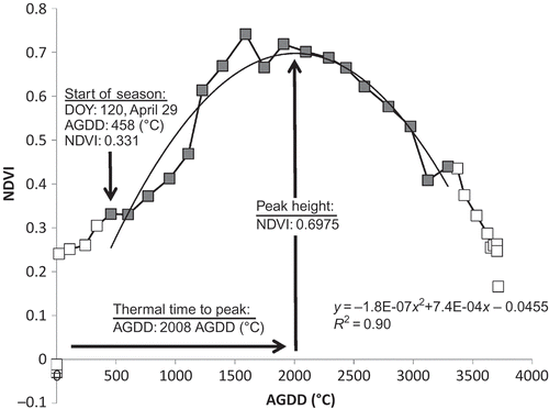
We started our phenological analysis by estimating the start and length of the growing season based on NDVI, with the midpoint pixel method (White et al., 2009). To characterize the remainder of the growing season, we used the quadratic method with AGDD as the dependent variable. We have previously shown that linking NDVI to AGDD using a quadratic function can provide a parsimonious well-fitting model for the land surface phenologies in similar cropland areas in Kazakhstan (de Beurs & Henebry, 2004). We have subsequently successfully applied the models in other northern latitudes (de Beurs & Henebry, 2008a, 2010a) as well as dryland crop areas in Africa (Brown & de Beurs, 2008; Brown, de Beurs, & Vrieling, 2010). These quadratic regression models have only three parameters to estimate, which yield straightforward ecological interpretations. Furthermore, these models can be applied directly to the data without the need of applying filters to remove noisy data. The basic quadratic regression model is in this form:

For each pixel, we calculated the average and standard deviation of the phenological metric based on all years (2002–2009). We hypothesized that the standard deviation calculated for each phenological metric over the 8 years represented in our study (2002–2009) would be higher for croplands than for natural vegetation as a result of crop-rotation schemes. In addition, we anticipated a difference in the start of the growing season, the peak height and the peak timing.

3.5. Cropland probability map

The effective resolution of the MODIS data is 463.3 meters. The spatial resolution of the Landsat data is 30 m. We resampled the annual phenological metrics to 450 m to ensure that we could have a whole number of Landsat pixels within each MODIS unit. We aggregated the Landsat data to 450 m, so that each 450 m pixel provided the percentage of cropland in that area. We then randomly selected 5000 pixels to generate a logistic model linking the availability of cropland within a pixel with the phenological metrics. The logistic model is as follows:

where x₁, … x_k are the phenological metrics. When a particular grid cell was found to have more than 50% of croplands, we set the dependent variable to 1; if less than 50%, we set the variable to zero. We applied step-wise regression to find the best-fitting model. The goodness-of-fit of the logistic regressions was assessed by the percentage of observations predicted correctly (PC), Cohen’s kappa and the area under the curve (AUC) of the receiver operating characteristic. Cohen’s kappa assesses the accuracy of location and PC describes the ratio of correctly predicted cells from the total number of cells. The AUC measures the performance of a model compared to a random model while the cut-off threshold is varied from zero to one (Pontius & Schneider, 2001).

After we found a statistically significant model, we applied the model to all pixels in both MODIS tiles. We evaluated the results by comparing the estimated number of hectares of arable land in each rayon in the study area with statistics from the All-Russia Agricultural Census. We also validated the data based on 721 random MODIS samples checked with Google Earth high-resolution data. It is important to note that pixels that were abandoned early in our time period but became reoccupied sometime during the period 2002–2009 will be identified as cropland as a result of increased temporal variability. In addition, pixels that were cropland early in our time period that were abandoned sometime during the period 2002–2009 will also be identified as cropland, as a result of increased temporal variability. In subsequent steps, we determined how often each cropland pixel is actually cropped.

3.6. Cropping intensity

To determine whether a pixel was successfully sown during a particular year, we applied a series of basic decision rules. In this section, we aim to distinguish between cropped pixels and fallow pixels within the general class of cropland. The fallow pixels can be fallow for multiple years, and thus have a variety of vegetation growing on them. However, the fallow pixels must have at least been cropped once during our study period, as identified above, to be counted as cropland. The phenology models tend to fail for clean fallow areas, thus we assumed that if the model failed to fit for a particular year, there were likely no crops in that pixel for that year. Failed models have either no values or lower than 0.4. Crops tend to peak sooner than vegetation growing on fallow fields; in addition, the NDVI during the peak of the growing season tends to be higher for crops than for vegetation growing on fallow fields. Thus, we identified the following rules and applied them to all pixels with a crop probability higher than 0.5:

1. If models fail → no crops.

2. If the peak height > μ peak height – σ peak height AND peak timing (in AGDD) < 1100AGDD → crops.

Where μ peak height (Figure 3) is the average of the peak heights per pixel based on the years 2001 through 2009, and σ peak height is the standard deviation of the peak heights per pixel for the same years. We have evaluated several cut-off degrees for AGDD and determined that a cut-off of 1100 generates the most accurate results. We validate the results against statistical yearbook data, indicating the number of hectares with successfully sown crops for each year separately between 2004 and 2008.

4. Results and discussion

4.1. Landsat classification

Table 2. Confusion matrix for the Landsat classification results of all seven path/row combinations

	Reference Data
		Water	Forest	Grassland	Cropland	Urban	Σ	UAC
Classified	Water	9862	222	41	0	283	10,408	0.948
	Forest	85	66,506	1216	349	602	68,758	0.967
	Grassland	70	2914	14,673	7510	1389	26,556	0.553
	Cropland	218	1227	2047	56,102	1406	61,000	0.920
	Urban	53	529	494	1028	7022	9126	0.769
	Σ	10,288	71,398	18,471	64,989	10,702	175,848
	PAC	0.959	0.931	0.794	0.863	0.656

Notes: Overall accuracy: 0.877; kappa coefficient: 0.821.

UAC, user’s accuracy; PAC, producer’s accuracy.

Figure 4 gives the resulting Landsat classification for the four path/row combinations covering Samara oblast. The combined confusion matrix for all seven path/row combinations can be found in Table 2. We provide the confusion matrix based on individual pixels, the results based on segments are comparable (not shown). The overall accuracy of the classified image is 0.877, with a kappa coefficient (K) of 0.82. The two classes with the lowest user accuracy are grassland (0.55) and urban areas (0.77); both are most often confused with cropland. In the case of urban areas, it is not surprising given the observations during our field work. There are a number of towns in our study region that show the typical pattern of urban agriculture with extensive garden networks within the town. We suspect that the confusion between grasslands and cropland is a result of sown meadows as well as a shift from croplands to meadows, and the subsequent reversion in some instances that occurs during the study period. To ensure the spatial stability of the classification result, we independently validated the path/row combinations in the three groups: the four tiles covering Samara oblast, the tile covering Chuvash Republic and the two tiles covering Kostroma oblast. The overall accuracy and kappa statistics for the groups were stable, with a slightly higher accuracy for the path/row covering Chuvash Republic (Table 3). We believe that the accuracy is slightly higher in Chuvash Republic because it is generally an active region with respect to agriculture. There are fewer abandoned areas than in Kostroma oblast and the agricultural fields are more regularly used for crops than in Samara oblast, where there are more frequent fallow periods.

Table 3. Overview of the Landsat classification accuracy for the three subregions

Path/row groups	Overall accuracy	Kappa coefficient
169/22, 169/23, 169/24, 170/23 – Samara Oblast	0.862	0.8017
172/22 – Chuvash Republic	0.946	0.8975
176/20, 174/19 – Kostroma Oblast	0.896	0.8249

Figure 4. Output of the Landsat classification for Samara oblast.

4.2. Phenology models

The average coefficient of determination (R²) of the quadratic phenology model linking AGDD and NDVI for all pixels in the two tiles and all years (2002–2009) was 0.83. More than 90% of the pixel/years revealed an R² above 0.75. The average start of the growing season for the two tiles was on April 12 (day 102). The average length of the growing season was 145 days. The length of the growing season was generally shorter in the south-eastern area of the tiles, close to the border and into Kazakhstan. Areas that were identified as croplands had later starts and shorter growing seasons. They also had lower average peak heights (NDVI) and their vegetative peak was reached for more AGDDs. In addition, the temporal variability of the phenological variables was higher for croplands than for other areas.

4.3. Cropland probability

Table 4 gives the parameter estimates for the cropland probability model. We used the aggregated Landsat data as the dependent variable and the average and standard deviation of the MODIS phenology results (per pixel average and standard deviation over 8 years) as the independent variable.

The cropland probability model reveals ten significant phenological variables besides the intercept: R², standard deviation of R², peak position (in AGDD), peak height, standard deviation of peak height, SOS, standard deviation of SOS, length of season, standard deviation of length of season and AGDD at SOS. In addition, the spatial location of the areas was significantly identified as X and Y, and was measured in meters. Based on the parameter estimates, we can calculate the odds ratios of a particular pixel being cropland. For example, the parameter estimate for R² (8.34) indicates that, holding all other variables at a fixed value, since exp (8.34 × 0.01) = 1.087, we will see an 8.7% increase in the odds of a pixel being cropland for a 0.01 increase in R². In a similar way, we can derive that an increase in the peak height of 0.01, while holding all other variables at a fixed value would result in a 5.8% increase in the odds of a pixel being cropland. Ten degrees increase in the thermal time to peak AGDD (°C), results in a 4.4% increase in the odds of a pixel being cropland. The parameter estimate for the length of the season indicates that, holding all other variables at a fixed value, we will see a 3.7% decrease in the odds of a pixel being cropland for a 1 day increase in the length of the season (exp(–0.43/16) = 0.973).

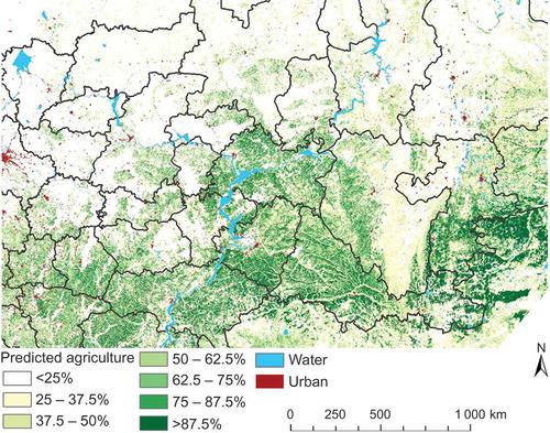
Table 4 also provides the goodness-of-fit logistic regression assessments for the cropland models. The percentage of observations predicted correctly was 78.7%. The area under the receiving curve reveals a very good fit (0.849). In general, the goodness-of-fit is satisfactory. Figure 5 provides the cropland estimations based on the logistic regression model. The cropland areas are found mainly in the southern part of the study region.

Table 4. Significant parameter estimates for the logistic regression model to identify cropland

Variable	Parameter estimate	S.E.
Constant	−8.75	1.87
	8.34	1.10
std. dev.	33.69	4.36
PP	4.33E-3	3.27E-4
Peak height	5.60	0.60
Peak height std. dev.	51.13	9.35
SOS	0.33	0.08
SOS std. dev.	4.14E-2	08.72E-3
LOS	−0.43	0.03
LOS std. dev.	2.00E-2	1.94E-3
AGDD at SOS	3.37E-3	9.78E-4
X (in meters)	2.88E-6	2.90E-7
Y (in meters)	8.68E-7	3.72E-7
Goodness-of-fit logistic regression assessments
PC		0.787
AUC		0.849
Cohen’s kappa		0.536

Notes: PC: percentage of the observations predicted correctly; AUC: area under the curve of the receiver operating characteristic.

Cohen’s kappa indicates that the model provides a moderately significant fit.

Figure 5. Predicted agriculture based on the logistic model developed in this article.

4.4. Cropland data comparison

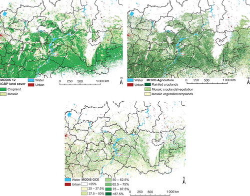
We compare our cropland probability map (Figure 5) with three global products that also provide cropland estimates (Figure 6). The first product (Figure 6a) is the MODIS IGBP land cover classification. This map shows a substantive amount of cropland in our study region. The second product (Figure 6b) is the MERIS 300 m Globcover data. There are three classes that incorporate croplands. The rainfed croplands class and the mosaic of croplands and vegetation dominate the land surface. The third product (Figure 6c) is the Global Cropland Extent which gives the cropland probability in a similar way as our own data set. This data set clearly depicts less cropland in the area than the other two data sets.

Figure 6. (a) MOD12 IGBP land cover map highlighting croplands only. (b) MERIS indicating three cropland classes. (c) Cropland probability according to the global cropland extent map by Pittman et al. (2010).

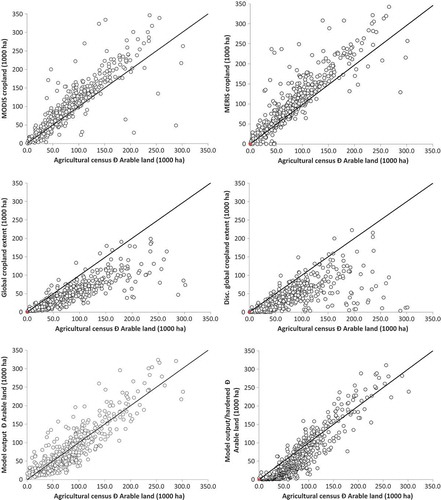
There are 22 oblasts and republics that fall entirely on our MODIS tile. Figure 7 shows the estimated cropland per rayon for all the 565 rayons in these 22 oblasts and republics in our study region. When we evaluate the accuracy of the cropland data layers, we not only look at and RMSE but we are also interested in how close the regression estimates are to a 1:1 line. We find that the MODIS cropland data slightly overestimate the amount of arable land for larger agricultural rayons, indicated by the points above the 1:1 line in Figure 7a. The MERIS data also slightly overestimate the amount of arable land in such rayons. However, MERIS data are generally closer to the 1:1 line. There is increased spread for rayons with more arable land and a slightly upward bias. The Global Cropland Extent data underestimates the amount of arable land for all rayons, both in the probability map and in the discrete map (Figure 7c and d). Almost all estimates fall well below the 1:1 line. Our model based on the original probabilities shows slightly more spread around the 1:1 line, but does not systematically overestimate or underestimate the amount of arable land (Figure 7e). Our model based on the hardened probabilities shows the best but slightly underestimates the amount of arable land in areas with less than 50,000 ha of arable land (Figure 7f). The regression estimates for all rayons combined and separated by oblast/republic for these analyses can be found in Table 5. The for our probability estimates, the MODIS IGBP estimates and the MERIS estimates are very similar (∼0.79 with RMSE of ∼27,000 ha). Our hardened results have a slightly higher (0.849). The for the Global Cropland Extent are worse (0.71 for the probability map and 0.42 for the discrete map). The slope estimates are perhaps the best way to compare these data sets. Both our cropland probability data and the MERIS data have slope estimates close to 1 (1.028 and 1.099, respectively). The MODIS IGBP data reveals a slightly higher slope of 1.143. The Global Cropland Extent data set significantly underestimates the amount of cropland and reveals a slope of 0.558 for the probability product and 0.443 for the discrete product. All the products reveal lots of variability among different oblasts as well. It is interesting to note that we find much higher for some oblasts for all products than for others. For example, the is relatively low for Ivanovo for all products (0.315–0.636), while the is high for all products for Chelyabinsk (0.832–0.943).

Figure 7. MODIS croplands, MERIS croplands, global cropland extent from Pittman et al. (2010) and our arable land estimates for all rayons incorporated in the study. Linear line is the 1:1 line. Model estimates are in Table 5.

Table 6 reveals the independent confusion matrix based on 721 MODIS pixels that overlaid high-resolution Google Earth imagery. The overall accuracy was about 0.70 for all three standard global products. The kappa values varied between a low of 0.28 for the MODIS cropland extend data, and a high of 0.44 for the MOD12 land cover product. Our cropland probability data had a higher accuracy (0.78) and a higher kappa (0.54) than any of the other data sets.

Our results confirm the work by Fritz et al. (2011) who found that MODIS data estimated more croplands in our study region than MERIS data. Careful validation of these and other cropland data sets over a range of cropland types based on ground observations as suggested by Fritz et al. (2011), and based on regional crop land statistics is necessary to get a better understanding of the accuracy of these data sets. The geo-wiki.org website, which forms the basis for the Fritz et al. (2011) and (2012) papers, does provide a comparison of cropland estimates with independent statistical data. For Russia, the land cover estimates are compared with the FAO arable data for 2000 and 2005. However, these estimates are currently country wide and not regional as we present here. We like to point out that our study is not able to make any claims about the relative accuracy of each data set in regions outside of the areas evaluated here.

Table 5. Regression results with agricultural census statistics

	MODIS logistic model				MODIS logistic model – hardened				MERIS LC data				MOD12 LC data					MODIS cropland extent				MODIS cropland extent – discrete
Regions	Int.	Sl.		RMSE	Int.	Sl.		RMSE	Int.	Sl.		RMSE	Int.	Sl.		RMSE	N	Int.	Sl.		RMSE	Int.	Sl.		RMSE
Bashkortostan	59.9	0.617	0.121	44.1	−34.6	1.485	0.842	18.2	25.1	1.335	0.382	48.2	5.5	1.575	0.588	37.0	48	−10.2*	0.958	0.697	17.8	−17.2	1.077	0.705	19.6
Chelyabinsk	19.4	1.075	0.943	22.0	−12.9*	1.224	0.931	27.7	6.6*	1.254	0.931	28.6	−2.8*	1.375	0.940	28.9	30	−4.7*	0.832	0.922	20.1	−6.5*	0.847	0.847	29.8
Chuvash	7.1*	0.455	0.583	4.1	1.9*	0.385	0.169	8.2	5.5*	0.893	0.811	4.6	6.7	0.910	0.828	4.4	21	3.8*	0.438	0.758	2.6	3.9*	0.501	0.461	5.6
Ivanovo	3.6*	0.439	0.532	3.0	−5.8*	0.351	0.332	3.5	6.2*	0.714	0.368	6.6	−5.5*	1.044	0.636	5.7	17	−0.7*	0.407	0.358	3.8	−5.6*	0.426	0.315	4.3
Kostroma	25.1	0.355	0.085	10.7	−1.0*	0.120	0.231	2.3	−18.7*	1.055	0.183	17.7	−11.5	1.059	0.634	9.0	10	0.4*	0.224	0.543	2.3	−0.6*	0.054	0.192	1.2
Kurgan	56.5	0.810	0.734	17.2	15.2*	0.960	0.635	25.5	79.2	0.828	0.607	23.2	58.5	0.894	0.716	19.8	24	13.2*	0.574	0.597	16.5	13.2*	0.585	0.516	19.7
Kursk	0.5*	0.533	0.595	7.4	−1.3*	0.461	0.267	12.4	0.0*	1.044	0.880	6.5	6.4*	1.029	0.901	5.8	27	−1.4*	0.550	0.884	3.4	−3.1*	0.485	0.607	6.6
Lipetsk	−5.6*	0.778	0.836	7.7	−11.5*	0.866	0.719	12.1	1.6*	1.077	0.872	9.3	3.7*	1.085	0.920	7.2	17	14.7	0.412	0.650	6.7	21.0	0.329	0.416	8.4
Mari-El	18.9	0.432	0.437	8.5	−4.8*	0.703	0.797	6.3	4.7*	0.973	0.701	11.3	9.5	0.997	0.786	9.6	14	6.2*	0.332	0.830	2.8	1.3*	0.377	0.867	2.7
Mordovia	4.3*	0.625	0.847	4.2	−3.0*	0.583	0.533	8.5	6.4*	1.030	0.664	11.5	3.0*	1.176	0.879	7.1	21	3.6*	0.541	0.789	4.4	3.7*	0.531	0.782	4.4
Nizhegorod	9.2	0.517	0.666	7.2	−5.7*	0.503	0.544	9.1	5.4*	0.927	0.513	17.6	−4.9*	1.219	0.828	11.0	43	−1.9*	0.523	0.741	6.2	−7.9	0.570	0.644	8.4
Orenburg	−6.6*	1.171	0.846	27.5	−4.5*	1.095	0.869	23.4	29.2	0.984	0.563	47.4	28.5*	0.991	0.309	79.1	33	39.6	0.328	0.231	31.5	69.1	−0.022	−0.031	43.5
Penza	0.4*	0.649	0.942	5.7	−18.0	0.683	0.765	13.3	21.9	0.891	0.916	9.5	11.1	0.993	0.924	10.1	26	4.6*	0.526	0.928	5.2	−0.1*	0.556	0.860	7.9
Ryazan	8.7*	0.465	0.674	9.7	−5.7*	0.472	0.576	12.1	39.7	0.734	0.380	27.4	23.7	0.937	0.692	18.7	25	15.1	0.420	0.623	9.8	17.1	0.334	0.446	11.0
Samara	−9.4*	1.062	0.926	11.0	−32.0	1.256	0.859	18.6	2.1*	1.118	0.900	13.7	−0.4*	1.135	0.920	12.3	25	1.2*	0.655	0.836	10.6	11.3*	0.584	0.610	16.9
Saratov	13.3*	0.796	0.833	22.0	−9.9*	0.939	0.808	26.6	62.6	0.716	0.630	33.8	35.3*	0.844	0.519	49.8	37	31.4	0.246	0.282	26.6	36.7	0.059	−0.017	35.1
Tambov	6.6*	0.691	0.763	10.0	−0.1*	0.781	0.475	20.9	22.8	0.925	0.795	12.2	28.3	0.836	0.785	11.4	22	13.4*	0.362	0.403	11.1	12.0*	0.325	0.335	11.5
Tatarstan	3.5*	0.981	0.782	10.8	−3.2*	1.056	0.793	11.2	15.6*	0.919	0.591	15.9	9.0*	1.083	0.751	13.0	40	3.3*	0.568	0.600	9.6	2.7*	0.679	0.533	13.1
Tula	−9.1*	0.575	0.688	7.6	−15.8*	0.510	0.372	12.6	−5.7*	1.055	0.948	4.8	−4.9	1.116	0.982	3.0	23	1.7*	0.500	0.893	3.4	6.4*	0.376	0.453	7.9
Udmurt	6.2*	0.718	0.793	7.3	−10.5*	0.672	0.500	13.1	7.2	0.874	0.820	8.1	1.0*	0.857	0.661	12.1	25	−1.4*	0.334	0.474	6.9	−3.9*	0.327	0.278	10.0
Ul’yanovsk	−8.5*	0.964	0.869	12.3	−26.3	1.039	0.752	19.5	12.4*	0.975	0.868	12.5	3.7*	1.091	0.916	10.9	21	2.0*	0.630	0.822	9.6	−6.7*	0.798	0.800	13.1
Vladimir	6.1	0.419	0.572	7.5	−7.6	0.387	0.703	5.2	36.8	0.562	0.116	26.6	−4.6	1.127	0.854	10.2	16	2.9*	0.480	0.841	4.4	−3.2*	0.480	0.800	5.0
All	−6.6	1.028	0.796	27.3	−27.7	1.135	0.849	24.6	8.3	1.099	0.785	30.1	3.6*	1.143	0.784	31.5	565	2.0	0.558	0.709	18.7	6.9	0.443	0.420	27.3

Notes: Int: intercept; Sl.: slope; RMSE: root mean square error; N: number of rayon in the region.

*Not significantly different from 0.

All parameter estimates are in 1000 ha.

4.5. Cropping intensity

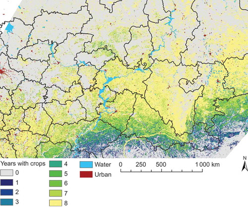
We are interested in estimating not only the number of hectares of arable land but also the cropping intensity. We define cropping intensity as the number of years a field is sown with crops and actually reaches harvest. The cropping intensity is influenced by both management decisions and droughts. Figure 8 reveals that the cropping intensity for our study region shows a north–south gradient with more intense cropping in northern regions, where fields are successfully sown 8 out of 8 years and less intensity in the southern areas, where crops are successfully sown as little as 1 or 2 out of 8 years. We compare the data with successfully sown statistics retrieved from the agricultural statistical books of Samara. We have data available for 5 years (2004–2008). All the years are tightly clustered, and the intercept for the combined regression line is not significantly different from 0, the combined regression line has a slope of 1.213 (Table 7). Table 7 indicates a slight overestimation of the successfully sown area for the high-agricultural rayons. This overestimation appears to be stronger for the earlier years (2004–2006), as the slope for the years 2007 and 2008 is not different from 1.

Table 6. Confusion matrix for the four different satellite products, including the data created by logistic models as presented in this article

	Google Earth reference data
		Cropland	Other	Σ	UAC	Accuracy	Kappa
MODIS logistic	Cropland	189	36	225	0.84
	Other	117	373	490	0.76
	Σ	306	415	721
	PAC	0.62	0.90			0.78	0.54
MODIS LC	Cropland	269	170	439	0.61
	Other	37	245	282	0.87
	Σ	306	415	721
	PAC	0.88	0.59			0.71	0.44
MODIS cropland extend	Cropland	91	16	107	0.85
	Other	215	399	614	0.65
	Σ	306	415	721
	PAC	0.30	0.96			0.70	0.28
MERIS	Cropland	231	136	367	0.63
	Other	76	279	354	0.79
	Σ	306	415	721
	PAC	0.75	0.67			0.71	0.42

Table 7. Regression statistics of the successfully sown analysis. Samara oblast only

	Successfully Sown Land
	Intercept	Slope		RMSE
2004	−11.451*	1.331	0.915	12.215
2005	−3.856*	1.189	0.906	11.732
2006	−3.944*	1.271	0.899	13.423
2007	6.984*	1.156**	0.857	14.979
2008	1.646*	1.160**	0.864	14.916
Overall	−1.457*	1.213	0.884	13.578

Notes: *Not significantly different from 0 (p = 0.05); **Not significantly different from 1 (p = 0.05).

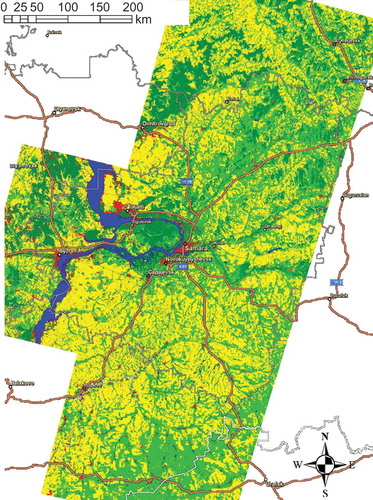
Figure 8. The number of years with crops between 2002 and 2009. Yellow pixels are cropped every year during the 8-year period from 2002–2009. Other colours indicate at least one fallow year during this period. There is a north–south gradient, with pixels in the south indicating more fallow years than northerly pixels.

Accurate crop type mapping is not a trivial task and requires a large amount of precise field observations (Wardlow & Egbert, 2008). In lieu of crop type mapping, we argue that a first step is to not only map cropland extent but also crop intensity. Crop intensity changes from the previously standard 7-year crop rotations (a variety of grain crops and 1 year of clean fallow) toward 3 or 4-year crop rotations which are focused on other crops than cereals may indicate a change of specialty for the Russian farmers. In addition, current climate conditions and the ongoing climate change may result in increased crop failures due to drought conditions. We are only aware of a few studies that mapped the cropland intensity over several years (Watts et al., 2011); however these studies were primarily based on Landsat data. One study mapping crop type with MODIS data also mapped fallow lands (Wardlow & Egbert, 2008) but they only investigated 1 year, and only focused on the Central Great Plains in the USA. Another study, only focusing on the Rostov region of Russia also incorporated fallow lands (Fritz et al., 2008). Others are interested in yield mapping and acknowledge variability in wheat fields, but (rightly) assume that the data are static at coarser resolution (Becker-Reshef, Vermote, Lindeman, & Justice, 2010).

In recent years, planting decisions have become largely market-based in most of Russia and Ukraine (Lindeman, 2004). As a result, crop production in Russia and the other countries of the former Soviet Union has shown a shift from mainly cereal to increased sunflower, soybean and rapeseed production. These three crops have increased in Russia from 5.6 to 11.9 million harvested hectares between 1990 and 2005 (European Bank for Reconstruction and Development, 2008). Sunflower has become one of the most consistently profitable crops in Russia and Ukraine. The production costs of sunflower are relatively low partly due to lower requirements of fertilizer and herbicide applications (Lindeman, 2004). The large leaf structure of sunflowers makes them great competitors for weeds. In addition, new investors are appearing in the area. FAO expects 13 million hectares of previously abandoned land to be returned to production and devoted to grain (European Bank for Reconstruction and Development, 2008) with the main increase in sunflower production to occur on newly re-cultivated land.

Crop rotation changes, including changes in the frequency of summer fallow and crop failures, are common in other global cereal belts as well. Our findings on crop intensity (Figure 8) are consistent with what can be found in other countries. For example, in 2002, which was a drought year in the United States, 4.4% of the crops in the United States failed, but this number was much higher in the wheat-growing regions of the Great Plains, e.g. 16% in Colorado, 11% in Texas (USDA Economic Research Service, 2005). In addition, there have been some marked changes in the use of summer fallow in the United States. In 1969, the amount of summer fallow was 41 million acres (almost 10% of the cropland area). The area of summer fallow dropped to just 19 million acres in 2002, mainly as a result of widespread adaptation of alternative tillage practices (USDA Economic Research Service, 2005). However, the amount of fallow lands is much higher in the wheat growing regions of the Great Plains. One study found that in western Kansas, producers have moved from a typical wheat/fallow rotation to rotations involving wheat and feed grains with fallow once every 3 years (Langemeier, 2012). Some producers are even adopting crop rotations that fallow once every 4 years. Changes in tillage practices (Zheng et al., 2012) from conventional tillage to reduced-till or conservation tillage have resulted in drastic changes in the crop intensity. The percentage of fallow has been changing in Canada as well, as a result of adaptation of alternative tillage practices. For example, in the early 1980’s and 1990’s, approximately half the cropland areas in Saskatchewan were set aside in summer fallow practices (Census Canada, 1991). This is comparable to the crop intensity we find in cereal growing regions in southern Samara and northern Saratov oblasts. In Canada, the amount of fallow land dropped to just 9.6% of the cropland by 2006 (Census Canada, 2006).

5. Conclusions

Several readymade data sets exist that estimate cropland (probability) extent on a global scale. We evaluated three of the most recent cropland layers against the 2006 All-Russia Agricultural Census data, and found that only the MERIS Globcover data resulted in cropland estimates closely comparable to independently collected statistics. The cropland estimate from the MODIS IGBP data set slightly overestimated the amount of cropland in our study region, while the MODIS Global Cropland Extent data significantly underestimated the amount of cropland in our study region. While the MERIS data resulted in acceptable estimates, we established our own cropland probability layer for the central grain belt in Russia, because we intended to use the MODIS information to create a cropland intensity data set as well.

To create the cropland probability, we used a combination of Landsat data and land surface phenology metrics estimated from MODIS time series. We have compared our results with the arable land estimates from the 2006 All-Russia Agricultural Census data set by rayon, and found that our data layer estimated the available cropland with sufficient accuracy. Our finely tuned data set performed slightly better than the MERIS GlobCover cropland estimates. We validated our cropland intensity data for 5 years (2004–2008) in the rayons of Samara oblast only, where we have statistical data on the amount of area successfully sown. Figure 8 shows that Samara is an appropriate region to validate the data because it falls in the middle of our study region. Even more importantly, it has rayons that were intensely cropped (up to 8 out of 8 years) in the North and rayons that were cropped far less frequently (4 out of 8 years). The areas south of Samara (e.g., Saratov) clearly show the result of droughts in the eastern area, especially showing pixels with crops as few as 2 out of 8 years.

To better understand changes in Russian agriculture, we cannot just look at the cropland extent. It is also necessary to understand the cropland intensity which is far from homogeneous over the region. In subsequent studies, we are interested in evaluating the cropland intensity’s correlation with climatological data to better understand the impact of drought. We are also interested in extending this data set in time, to incorporate 2010 which resulted in massive droughts over this study region, and in space, to incorporate all agricultural areas in European Russia.

Cropland percentage and intensity data can be found on our website (http://tethys.dges.ou.edu/main/?p = 223) and on the NASA Earth Exchange (NEX) webpage: https://c3.nasa.gov/nex/projects/227/.

Acknowledgement

The authors thank P. de Beurs for the application development that allowed them to estimate the land surface phenology data efficiently. They also thank two anonymous reviewers for their useful and thoughtful comments to an earlier version of this manuscript.

This research was supported in part by the NEESPI and NASA LCLUC project Land Abandonment in Russia: Understanding Recent Trends and Assessing Future Vulnerability and Adaptation to Changing Climate and Population Dynamics.

References

- Becker-Reshef, I., Vermote, E., Lindeman, M., & Justice, C. (2010). A generalized regression-based model for forecasting winter wheat yields in Kansas and Ukraine using MODIS data. Remote Sensing of Environment, 114, 1312–1323.
- Bontemps, S., Defourny, P., Van Bogaert, E., Arino, O., Kalogirou, V., & Perez, J. R. (2011). GlobCover 2009. Products description and validation report. ESA. Retrieved from http://dup.esrin.esa.it/files/p68/GLOBCOVER2009_Validation_Report_2.2.pdf
- Brown, M. E., & de Beurs, K. M. (2008). Evaluation of multi-sensor semi-arid crop season parameters based on NDVI and rainfall. Remote Sensing of Environment, 112, 2261–2271.
- Brown, M. E., de Beurs, K., & Vrieling, A. (2010). The response of African land surface phenology to large scale climate oscillations. Remote Sensing of Environment, 114, 2286–2296.
- Canty, M. J. (2010). Image analysis, classification and change detection in remote sensing, with algorithms for ENVI/IDL (2nd ed.). Boca Raton, FL: CRC Press.
- Census Canada. (1991). Agricultural Profile of Saskatchewan, Statistics Canada, Agriculture Division.
- Census Canada. (2006). Census of Agriculture 2006, Statistics Canada, Agriculture Division.
- Comaniciu, D., & Meer, P. (2002). Mean shift: A robust approach toward feature space analysis. IEEE Transactions on Pattern Analysis and Machine Intelligence, 24, 603–619.
- de Beurs, K. M., & Henebry, G. M. (2004). Land surface phenology, climatic variation, and institutional change: Analyzing agricultural land cover change in Kazakhstan. Remote Sensing of Environment, 89, 497–509. doi:410.1016/j.rse.2003.1011.1006
- de Beurs, K. M., & Henebry, G. M. (2005a). Land surface phenology and temperature variation in the IGBP high-latitude transects. Global Change Biology, 11, 779–790.
- de Beurs, K. M., & Henebry, G. M. (2005b). A statistical framework for the analysis of long image time series. International Journal of Remote Sensing, 26, 151–1573.
- de Beurs, K. M., & Henebry, G. M. (2008a). Northern annular mode effects on the land surface phenologies of northern Eurasia. Journal of Climate, 21, 4257–4279.
- de Beurs, K. M., & Henebry, G. M. (2008b). War, drought, and phenology: Changes in the land surface phenology of Afghanistan since 1982. Journal of Land Use Science, 3, 95–111.
- de Beurs, K. M., & Henebry, G. M. (2010a). A land surface phenology assessment of the northern polar regions using MODIS reflectance time series. Canadian Journal of Remote Sensing, 36, S87–S110.
- de Beurs, K. M., & Henebry, G. M. (2010b). Spatio-temporal statistical methods for modeling land surface phenology. In I. L. Hudson & M. R. Keatley (Eds.), Phenological research: Methods for environmental and climate change analysis (pp. 177–208). New York, NY: Springer.
- Dronin, N. M., & Bellinger, E. G. (2005). Climate dependence and food problems in Russia, 1900–1990: The interaction of climate and agricultural policy and their effect on food problems. Budapest: Central European University Press.
- European Bank for Reconstruction and Development. (2008). Fighting food inflation through sustainable investment, FAO.
- Friedl, M. A., Sulla-Menashe, D., Tan, B., Schneider, A., Ramankutty, N., Sibley, A., & Huang, X. M. (2010). MODIS collection 5 global land cover: Algorithm refinements and characterization of new datasets. Remote Sensing of Environment, 114, 168–182.
- Fritz, S., Massart, M., Savin, I., Gallego, J., & Rembold, F. (2008). The use of MODIS data to derive acreage estimations for larger fields: A case study in the south-western rostov region of Russia. International Journal of Applied Earth Observation and Geoinformation, 10, 453–466.
- Fritz, S., McCallum, I., Schill, C., Perger, C., See, L., Schepaschenko, D., … Obersteiner, M. (2012). Geo-Wiki: An online platform for improving global land cover. Environmental Modelling & Software, 31, 110–123.
- Fritz, S., See, L., et al. (2011). Highlighting continued uncertainty in global land cover maps for the user community. Environmental Research Letters, 6(4).
- Henebry, G. M., de Beurs, K. M., & Gitelson, A. A. (2005). Land surface phenologies of Uzbekistan and Turkmenistan between 1982 and 1999. Arid Ecosystems, 11, 25–32.
- Hölzel, N., Haub, C., Ingelfinger, M. P., Otte, A., & Pilipenko, V. (2002). The return of the steppe – large-scale restoration of degraded land in southern Russia during the post-soviet era. Journal for Nature Conservation, 10, 75–85.
- Ioffe, G. (2005). The downsizing of Russian agriculture. Europe-Asia Studies, 57, 179–208.
- Ioffe, G., Nefedova, T., & Zaslavsky, I. (2004). From spatial continuity to fragmentation: The case of Russian farming. Annals of the Association of American Geographers, 94, 913–943.
- Kuemmerle, T., Hostert, P., Radeloff, V. C., Perzanowski, K., & Kruhlov, I. (2007). Post-socialist forest disturbance in the Carpathian border region of Poland, Slovakia, and Ukraine. Ecological Applications, 17, 1279–1295.
- Kuemmerle, T., Radeloff, V. C., Perzanowski, K., & Hostert, P. (2006). Cross-border comparison of land cover and landscape pattern in eastern Europe using a hybrid classification technique. Remote Sensing of Environment, 103, 449–464.
- Lal, R. (2004). Carbon sequestration in soils of central Asia. Land Degradation & Development, 15, 563–572.
- Langemeier, M. (2012). Trends in Kansas wheat production. Kansas State Department of Agricultural Economics.
- Lasco, R. D., Ogle, S. M., Raison, J., Verchot, L., Wassman, R., Yagi, K., … Zhakata, W. (2006). 2006 IPCC guidelines for national greenhouse gas invetories. Vol. 4 Agriculture, Forestry and Other Land Use.
- Laykam, K. (2006), General overview of the 2006 All-Russia Agricultural Census procedure, design and content, Fourth international conference on agricultural statistics.
- Lindeman, M. (2003). Russia: Agricultural overview. Production Estimates and Crop Assessment Division Foreign Agricultural Service, FAS USDA.
- Lindeman, M. (2004). Sunflower seed production in Ukraine and Russia. Production Estimates and Crop Assessment Division Foreign Agricultural Division, FAS USDA.
- Lindeman, M. (2005). Ukraine: Agricultural overview, Production Estimates and Crop Assessment Division Foreign Agricultural Service, FAS USDA.
- Lobell, D. B., & Asner, G. P. (2004). Cropland distributions from temporal unmixing of MODIS data. Remote Sensing of Environment, 93, 412–422.
- Lokupitiya, E., Denning, S., Paustian, K., Baker, I., Schaefer, K., Verma, S., … Fischer, M. (2009). Incorporation of cropl phenology in Simple Biosphere Model (SiBcrop) to improve land-atmosphere carbon exchanges from croplands. Biogeosciences, 6, 969–986.
- Lucht, W., Prentice, I. C., Myneni, R. B., Sitch, S., Friedlingstein, P., Cramer, W., … Smith, B. (2002). Climatic control of the high-latitde vegetation green trend and Pinatubo effect. Science, 296, 1687–1689.
- Lucht, W., Schaaf, C. B., & Strahler, A. H. (2000). An algorithm for retrieval of albedo from space using semiemperical BRDF models. IEEE Transactions of Geoscience and Remote Sensing, 38, 977–998.
- Lunetta, R. S., Congalton, R. G., Fenstermaker, L. K., Jensen, J. R., McGwire, K. C., & Tinney, L. R. (1991). Remote-sensing and geographic information-system data integration – error sources and research issues. Photogrammetric Engineering and Remote Sensing, 57, 677–687.
- Pallot, J., & Nefedova, T. (2007). Russia’s unknown agriculture: Household production in post-soviet Russia. Oxford: Oxford University Press.
- Pflugmacher, D., Krankina, O. N., Cohen, W. B., Friedl, M. A., Sulla-Menashe, D., Kennedy, R. E., … Kharuk, V. I. (2011). Comparison and assessment of coarse resolution land cover maps for northern Eurasia. Remote Sensing of Environment, 115, 3539–3553.
- Pittman, K., Hansen, M. C., Becker-Reshef, I., Potapov, P. V., & Justice, C. O. (2010). Estimating global cropland extent with multi-year MODIS data. Remote Sensing, 2, 1844–1863.
- Pontius, R. G., & Schneider, L. C. (2001). Land-cover change model validation by an ROC Method for the Ipswich Watershed, Massachusetts, USA. Agriculture Ecosystems & Environment, 85, 239–248.
- Ramankutty, N., Evan, A. T., Monfreda, C., & Foley, J. A. (2008). Farming the planet: 1. Geographic distribution of global agricultural lands in the year 2000. Global Biogeochemical Cycles, 22, 1–19.
- Rast, M., Bezy, J. L., & Bruzzi, S. (1999). The ESA medium resolution imaging spectrometer MERIS – a review of the instrument and its mission. International Journal of Remote Sensing, 20, 1681–1702.
- Rembold, F., & Maselli, F. (2006). Estimation of inter-annual crop area variation by the application of spectral angle mapping to low resolution multitemporal NDVI images. Photogrammetric Engineering & Remote Sensing, 72, 55–62.
- Richards, J. A., & Jia, X. (2006). Remote sensing digital analysis: An introduction (4th ed.). Berlin: Springer.
- Rosenfield, G. H., & Fitzpatricklins, K. (1986). A coefficient of agreement as a measure of thematic classification accuracy. Photogrammetric Engineering and Remote Sensing, 52, 223–227.
- Rounsevell, M. D. A., Pedroli, B., Erb, K.-H., Gramberger, M., Busck, A. G., Haberl, H., … Wolfslehner, B. (2012). Challenges for land system science. Land Use Policy, 29, 899–910.
- Stanislav, F., Jonsson, H., Kust, G., & Zetterquist, F. (2010). Social and Environmental Assessment Report V.1 – social and environmental assessment (risks and possibilities). Volga Farming – Grain Production Project in Penza region (Russian Federation), Penza – Moscow, Russian Federation.
- Suleimenov, M., Akhmetov, K., Kaskarbayev, Z., Kireyev, A., Martynova, L., & Medeubayev, R. (2005). Role of wheat in diversified cropping systems in dryland agriculture of central Asia. Turkish Journal of Agriculture and Forestry, 29, 143–150.
- USDA Economic Research Service. (2005). Land use, value, and management: Major uses of land. Retrieved from http://www.ers.usda.gov/briefing/landuse/majorlandusechapter.htm
- Wardlow, B. D., & Egbert, S. L. (2008). Large-area crop mapping using time-series MODIS 250 M NDVI data: An assessment for the US central great plains. Remote Sensing of Environment, 112, 1096–1116.
- Watts, J. D., Powell, S. L., Lawrence, R. L., & Hilker, T. (2011). Improved classification of conservation tillage adoption using high temporal and synthetic satellite imagery. Remote Sensing of Environment, 115, 66–75.
- White, M. A., de Beurs, K., Didan, K., Inouye, D., Richardson, A., Jensen, O., … Lauenroth, W. (2009). Intercomparison, interpretation and assessment of spring phenology in North America estimated from remote sensing for 1982 to 2006. Global Change Biology, 15, 2335–2359.
- Zheng, B., Campbell, J. B., & de Beurs, K. M. (2012). Remote sensing of crop residue cover using multi-temporal Landsat imagery. Remote Sensing of Environment, 117, 177–183.