Recent land-use/land-cover change in the Central California Valley

Abstract

Open access to Landsat satellite data has enabled annual analyses of modern land-use and land-cover change (LULCC) for the Central California Valley ecoregion between 2005 and 2010. Our annual LULCC estimates capture landscape-level responses to water policy changes, climate, and economic instability. From 2005 to 2010, agriculture in the region fluctuated along with regulatory-driven changes in water allocation as well as persistent drought conditions. Grasslands and shrublands declined, while developed lands increased in former agricultural and grassland/shrublands. Development rates stagnated in 2007, coinciding with the onset of the historic foreclosure crisis in California and the global economic downturn. We utilized annual LULCC estimates to generate interval-based LULCC estimates (2000–2005 and 2005–2010) and extend existing 27 year interval-based land change monitoring through 2010. Resulting change data provides insights into the drivers of landscape change in the Central California Valley ecoregion and represents the first, continuous, 37 year mapping effort of its kind.

Keywords:

• agriculture
• land-use change
• change detection
• satellite imagery
• drivers of change

1. Introduction

Land-use and land-cover (LULC) data describe the earth’s surface at a given moment in time and can be used to identify underlying processes that have contributed to the current landscape. Biotic and abiotic interactions directly impact landscape patterns and potential (Bolliger, Wagner, & Turner, 2007; Turner, 2005), and indirectly determine how humans interact with their surroundings. Overlying these in situ processes are local, regional, and global socioeconomic and political factors which can also influence LULC and related decision-making processes. In order to understand how these biophysical and human components interact to influence land change, multiple ‘snapshots’ of LULC over time are required. Development of long-term land-use and land-cover change (LULCC) records facilitates exploration into the drivers of land change, especially in economically important regions with intensive land-use practices and dynamic change processes.

The Central California Valley ecoregion’s agriculture-based economy, rapidly expanding population, intensive land management, and existing historical LULCC inventory (Sleeter, 2008) make it a useful test area for analyzing modern land change. The Central California Valley has led the nation in agricultural production for over 50 years, contributing to California’s standing as the eighth largest economy in the world. The region sustains numerous cropping practices and produces a varied suite of agricultural commodities and specialty products. Population growth here has been rapid, outpacing the rest of California (U.S. Census Bureau, 2011). By 2010, the valley was home to nearly 7 million residents. Population pressures and intense agricultural land use have led to habitat fragmentation (Ferranto et al., 2011) and impacted both groundwater (California Regional Water Quality Control Board, 2010) and surface water quality (Lee & Jones-Lee, 2002) in the region. LULCC monitoring from 1973 to 2000 estimated that 5700 km² (12.4%) of the ecoregion experienced change, with agriculture increasing by 360 km² and developed lands increasing by 1100 km² (40%) (Sleeter, 2008). Sleeter (2008) also identified a 560 km² drought-induced loss in agriculture between the 1986 and 1992 interval of analysis.

Our objective was to extend existing LULCC records for the Central California Valley ecoregion through to 2010, comparing current land change dynamics to previously reported historical LULCC (Sleeter, 2008). By adding dates to the historical LULC record, we increase the temporal record of LULCC monitoring to nearly 40 years. We also explore the benefits and drawbacks of using annual versus interval-based estimates of land change. Implementing interval-based approaches to monitor LULCC has proven to be effective at capturing longer-term drivers of change such as shifting crop demand, multiyear drought, and overall population trends (Sleeter, 2008). We hypothesize that an annual analysis of LULCC will better capture localized LULC response to short-term, immediate drivers of change, such as water availability, modified policies, and/or economic instability. Determining LULC response to short-term drivers of change will improve understanding of local and regional landscape change processes, leading to more informed land management decisions.

1.1. Background

LULCC research is an important component in constructing a historical foundation from which long-term monitoring can extend (Lambin et al., 2001). Updating existing land-cover databases helps maintain the value of existing and expensive information (Smits & Annoni, 1999), and enables change detection analysis. The United States Geological Survey (USGS) Science Strategy (U.S. Geological Survey, 2007) recommends that global change research relies on existing ‘decades of observational data and long-term records to interpret consequences of climate variability and change to the nation’s biological populations, ecosystems, and land and water resources.’ The Intergovernmental Panel on Climate Change calls for estimating carbon and greenhouse gas emissions, including modeling frameworks where land-use change can be spatially tracked over time (IPCC, 2007). Updating existing LULCC studies using a consistent remote-sensing baseline can also provide a longer time frame for demonstrating spatial and temporal variability (Cousins, 2001), for identifying driving forces behind landscape change (Napton, Auch, Headley, & Taylor, 2010), and as validation in LULC forecasting efforts (Sohl, Loveland, Sleeter, Sayler, & Barnes, 2010). The key is to define operational, well-tested methodologies for long-term LULC monitoring and analysis.

Remote-sensing change detection is a proven, cost-effective method of creating LULC inventories and monitoring land change over time (Coppin, Jonckheere, Nackaerts, Muys, & Lambin, 2004; Fry et al., 2011). One of the most comprehensive LULCC studies was the USGS Land Cover Trends project (Loveland et al., 2002). This national LULCC detection effort used a sample and interval-based approach to estimate land change between 1973 and 2000 for all 84 Level III ecoregions (Omernik, 1987; U.S. Environmental Protection Agency, 1999) in the conterminous United States. The ecoregion framework was chosen because each region represents an area with similar human and biophysical processes influencing LULC distributions and potential landscape change. Intervals spanning 6–8 years were selected as an appropriate temporal scale to monitor regional-scale LULCC processes with moderate-resolution Landsat imagery. An interval-based temporal design was also selected due to finite project funding and high cost of Landsat satellite imagery at the time. Results of the Land Cover Trends project for the Central California Valley were presented in Sleeter (2008).

Underlying ecological processes and drivers of LULCC operate at various temporal scales (Turner, Gardner, & O’Neill, 2001) and can be missed using a multiyear interval approach. Temporal resolution, or repeat cycle, of change detection studies must be able to capture land changes as they occur. It is critical to fully understand the characteristic temporal variability of the LULC process in order to determine the driving forces behind LULCC (Phinn, Stow, Franklin, Mertes, & Michaelsen, 2003). For example, Sleeter’s (2008) identification of drought-induced losses of agriculture would not have been discernible given a single-year shift in the start or end year of his interval-based analysis.

Remote sensing-based studies of LULCC have focused on intra-annual, interannual, and interval-based (also referred to as multiyear or ‘book-end’) change. Intra-annual research often focuses on phenological or growing season changes (Zhang et al., 2003), while interannual studies vary in duration. In general, improved temporal resolution requires coarser image resolution, due to cost constraints (Phinn et al., 2003). Simply having long temporal intervals can be informative for analyzing trends in natural land cover, but are limited in the ability to describe biologically complex systems, specific driving forces, and anthropogenic land use operating on shorter timescales (Phinn et al., 2003). Human-induced changes often occur more rapidly, in which case, shorter temporal intervals may be more appropriate. Higher temporal frequency (Coppin et al., 2004) is a key component for identifying both LULCC drivers and resulting consequences such as changes in greenhouse gas emissions, climate feedbacks, and ecosystem resilience.

Higher classification accuracies have been shown where short, biennial-to-triennial time intervals were used (Coppin et al., 2004; Lambin, 1996). The temporal frequency of Landsat affords the opportunity to study a given area upwards of 22 times per calendar year at moderate spatial resolution (30 m pixels). Considerable progress has been made in monitoring change at a high frequency using stacks of Landsat images (Li et al., 2009; Roy et al., 2010). For large-scale LULCC analyses, annual profiles of LULC can capture change between years while limiting classification inaccuracies associated with phenological effects (Coppin et al., 2004; Goward, Masek, William, Irons, & Thompson, 2001). With Landsat imagery now available for free online, the cost of creating LULCC estimates at higher temporal resolution is greatly reduced.

Here, we present estimates of annual LULCC for the Central California Valley ecoregion from 2005 to 2010 using annual Landsat data and following the methodology used in the Land Cover Trends project (Figure 1). The temporal interval was adjusted to investigate annual change dynamics to better understand LULCC processes and drivers. By reproducing the Land Cover Trends methodology on a shorter timescale, we extended existing landscape change estimates to include six new annual LULC dates (2005., 2006, 2007, 2008, 2009, and 2010), adding two new temporal intervals (2005–2010, 2000–2005) to the existing interval-based 1973–2000 analysis. We investigate how annual estimates compare to temporal interval estimates, considering the highly variable LULC in the ecoregion. Leveraging previous change detection efforts in the Central California Valley has afforded us the opportunity to maintain the continuity of a long-term LULC record and extend change estimates from 27 to 37 years.

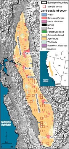
Figure 1. Sample data consist of 48 sample blocks randomly distributed throughout the Central California Valley Level III ecoregion (US Environmental Protection Agency, 1999)). Land-use/land-cover data are from the 2006 National Land Cover Data set (Fry et al., 2011) (mech. is mechanically, nonmech. is nonmechanically). The samples used in the current analysis are the same samples examined by Sleeter (2008). Projection is Albers Conical Equal Area.

2. Materials and methods

We followed the methods used by the US Geological Survey’s Land Cover Trends project, which characterized landscape change from 1973 to 2000 across all 84 Environmental Protection Agency (EPA) Level III ecoregions in the conterminous United States (U.S. Environmental Protection Agency, 1999). The project used a regionalized, pure panel random sampling approach and 10 km × 10 km sample blocks for interval-based LULCC analysis (Loveland et al., 2002: Stehman, Sohl, & Loveland, 2003), where the same samples were used for each date in the analysis. For the Central California Valley ecoregion, 48 sample blocks were randomly selected from a gridded population of 458 m available blocks. Manually interpreted LULC maps and LULCC estimates were produced for five image dates (1973., 1980, 1986, 1992, and 2000) and four discrete temporal intervals (1973. to 1980, 1980 to 1986, 1986 to 1992, and 1992 to 2000) (Sleeter, 2008). We produced annual LULCC estimates for the same 48 sample blocks from 2005 to 2010. We effectively mapped nearly 10% of the Central California Valley ecoregion and our random sampling included sample blocks in all of the counties in the study area. Here, we present six new annual LULC classification dates (2005., 2006, 2007, 2008, 2009, and 2010) and two new multiyear intervals (2000–2005, 2005–2010) and discuss the implications of varying temporal analysis in determining driving forces of LULCC.

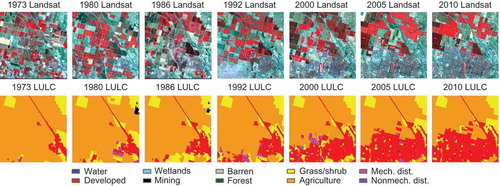
A team of five trained interpreters, following methods outlined by Loveland et al. (2002), mapped LULC in sample blocks using manual classification of Landsat TM satellite imagery. Summer scenes were selected for each year to limit classification inaccuracies associated with seasonality. All features with a footprint greater than 60 m × 60 m were classified into 11 general LULC classes based on the Anderson classification scheme (Anderson, Hardy, Roach, & Witmer, 1976; Table 1). Each annual LULC sample block was evaluated by a national team of reviewers, and directly compared to the previous sample block interpretations used in Sleeter (2008) to minimize mapping inconsistencies and enable comparison between results (Figure 2). Estimates of change and associated statistical uncertainties were calculated using post-classification analysis of LULC for each interpreted image date. In the prior effort, historical aerial photographs and topographic maps served as primary ancillary data sources to aid in image interpretation. In the current effort, we were able to utilize imagery (1995–2009) available through Google Earth, greatly reducing interpretation processing time by providing temporally consistent, easily comparable, readily accessible, ancillary data.

Table 1. The classification scheme follows a modified Anderson Level I classification and consists of 11 general LULC classes

Class	Description
Water	Areas persistently covered with water, such as streams, canals, lakes, reservoirs, bays, or oceans.
Developed/urban	Areas of intensive use with much of the land covered with structures (e.g., high-density residential, commercial, industrial, transportation, mining, confined livestock operations), or less intensive uses where the land-cover matrix includes both vegetation and structures (e.g., low-density residential, recreational facilities, cemeteries, etc.), including any land functionally attached to the urban or built-up activity.
Mechanically disturbed*	Land in an altered and often nonvegetated state that, due to disturbances by mechanical means, is in transition from one cover type to another. Mechanical disturbances include forest clear-cutting, earthmoving, scraping, chaining, reservoir drawdown, and other similar human-induced changes.
Barren	Land comprised of natural occurrences of soils, sand, or rocks where less than 10% of the area is vegetated.
Mining	Areas with extractive mining activities that have a significant surface expression. This includes (to the extent that these features can be detected) mining buildings, quarry pits, overburden, leach, evaporative, tailing, or other related components.
Forests/woodlands	Tree-covered land where tree-cover density is greater than 10%. Note that cleared forest land (i.e., clear-cut logging) will be mapped according to current cover (e.g., disturbed or transitional, shrubland/grassland).
Grassland/shrubland	Land predominately covered with grasses, forbs, or shrubs. Vegetated cover must comprise at least 10% of the area.
Agriculture	Cropland or pastureland in either a vegetated or nonvegetated state used for the production of food and fiber. Note that forest plantations are considered as forests or woodlands regardless of the use of wood products.
Wetland	Lands where water saturation is the determining factor in soil characteristics, vegetation types, and animal communities. Wetlands are comprised of water and vegetated cover.
Nonmechanically disturbed*	Land in an altered and often nonvegetated state that, due to disturbances by nonmechanical means, is in transition from one cover type to another. Nonmechanical disturbances are caused by wind, floods, fire, animals, and other similar phenomena.
Ice/snow	Land where accumulation of snow and ice does not completely melt during the summer period.

Note: *Indicates category included to capture anthropogenic or natural disturbance events.

Figure 2. An example of seven dates of Landsat imagery and corresponding LULC data for a sample block located on the edge of Bakersfield, CA. LULC maps not shown include 2006, 2007, 2008, and 2009.

3. Results

In 2010, the Central California Valley ecoregion, covering approximately 45,800 km², was primarily made up of four dominant LULC classes: agriculture, grassland/shrubland, developed, and wetland (Table 2). Combined, these four classes cumulatively make up over 98% of the ecoregion. We estimate that agricultural land use comprised roughly 32,700 km², or 71%, of the ecoregion. Grasslands/shrublands comprised an estimated 6800 km² of ecoregion, followed by development (4600. km²) and wetlands (roughly 1000 km²). Changes in these major LULC classes dominate the story of change in the Central California Valley ecoregion. Developed (increasing trend) and grassland/shrubland (decreasing trend) had the most significant linear trends over the study period (P < 0.05) based on parametric and nonparametric tests.

3.1. Annualized LULCC (2005–2010)

Applying an interval-based approach to the LULCC estimates can underrepresent change occurring at shorter temporal scales, especially in pixels changing more than once within a given interval. Annual LULC maps of the Central California Valley ecoregion were compared to calculate annual change estimates for the study area (Table 3). The annual rate of change was highest from 2005 to 2006 (1.1% per year), marked by fluctuations between grasslands/shrublands and agriculture, rapid rates of development, higher than normal changes in the wetland footprint across the region, and grassland/shrubland succession following fire. Slower development rates and reduced conversions between grasslands/shrublands and agriculture largely contributed to the low rate of estimated change from 2008 to 2009 and from 2009 to 2010.

Table 2. LULC composition and corresponding standard error reported as percentages of the Central California Valley ecoregion

		LULC class
Yearly composition		Water	Developed	Mech. dist.	Mining	Forest	Grass/shrub	Agriculture	Wetland	Nonmech. dist.
2000	Estimate (%)	1.0	9.3	0.2	0.1	0.4	15.5	71.8	1.8	0.0
	Std. Err (%)	0.3	2.6	0.1	0.1	0.1	3.1	3.8	0.8	0.0
2005	Estimate (%)	1.0	9.8	0.1	0.1	0.4	15.0	71.4	2.0	0.2
	Std. Err (%)	0.4	2.7	0.0	0.1	0.1	3.0	3.9	0.8	0.1
2006	Estimate (%)	1.1	10.0	0.1	0.1	0.4	15.0	71.4	2.0	0.0
	Std. Err (%)	0.4	2.8	0.0	0.1	0.1	3.0	3.8	0.8	0.0
2007	Estimate (%)	0.9	10.0	0.1	0.1	0.4	14.9	71.4	2.2	0.0
	Std. Err (%)	0.3	2.8	0.0	0.1	0.1	3.0	3.8	0.8	0.0
2008	Estimate (%)	0.9	10.1	0.1	0.1	0.4	15.1	71.1	2.2	0.0
	Std. Err (%)	0.3	2.8	0.0	0.1	0.1	3.1	3.9	0.8	0.0
2009	Estimate (%)	1.0	10.1	0.1	0.1	0.4	15.0	71.2	2.2	0.0
	Std. Err (%)	0.3	2.8	0.0	0.1	0.1	3.1	3.9	0.8	0.0
2010	Estimate (%)	1.0	10.1	0.0	0.1	0.4	14.8	71.3	2.1	0.0
	Std. Err (%)	0.4	2.8	0.0	0.1	0.1	3.0	3.9	0.8	0.0

Table 3. Percent of the Central California Valley ecoregion that underwent change each year between 2005 and 2010, including confidence interval, standard error, and relative error of estimated change

Period	Eco change %	85% +/–	Standard error (%)	Relative error (%)
2005–2006	1.1	0.4	0.3	24.5
2006–2007	0.7	0.3	0.2	23.8
2007–2008	0.9	0.6	0.4	45.8
2008–2009	0.5	0.2	0.1	22.8
2009–2010	0.6	0.3	0.2	36.1

Between 2005 and 2010, changes in many LULC types were dynamic, marked by high interannual variability rather than uniform rates of change (Table 4). Agriculture and grassland/shrubland underwent the most annual fluctuations in footprint across the Central California Valley ecoregion over this period. For agriculture, per interval net change was generally stable with the exception of a 139 km²/year net decline for 2007–2008 and a 77 km²/year net gain for 2009–2010. Trends in agriculture tended to have an inverse influence on grasslands/shrublands. However, when agriculture stabilized in 2005–2006, 2006–2007, and 2008–2009, persistent losses in grasslands/shrublands were largely attributable to conversions to development. Gains in new development were highest between 2005 and 2006, but slowed steadily in each of the following years. Ultimately the annual approach more clearly identifies fluctuations in LULCC, which can be masked using a wider interval.

Table 4. Average annual gains and losses by land-use/land-cover class for the Central California Valley ecoregion (2005–2010)

Normalized gains and losses (km²/year)	2005–2006	2006–2007	2007–2008	2008–2009	2009–2010
Water
Gains	45	12	14	47	48
Losses	−27	−79	−27	−11	−39
Net (gains minus losses)	18	−67	−14	36	9
Developed
Gains	63	27	19	20	12
Losses	−	−	−	−	−
Net	63	27	19	20	12
Mechanical disturbance
Gains	28	26	12	24	11
Losses	−25	−19	−18	−21	−25
Net	4	7	−6	3	−13
Nonmechanical disturbance
Gains	18	7	8	0	2
Losses	−86	−18	−7	−8	<−1
Net	−68	−11	1	−8	2
Forest
Gains	−	−	−	−	−
Losses	−1	<−1	−	0	−
Net	−1	<−1	−	0	−
Grass/shrubland
Gains	139	75	229	33	53
Losses	−175	−122	−105	−78	−140
Net	−35	−47	124	−46	−86
Agriculture
Gains	143	102	92	69	117
Losses	−153	−80	−232	−56	−40
Net	−10	22	−139	13	77
Mining
Gains	1	1	<1	<1	−
Losses	<−1	−1	−1	<−1	<−1
Net	<1	<1	<−1	<1	−1
Wetland
Gains	74	77	14	31	28
Losses	−46	−11	−12	−38	−37
Net change	28	66	2	−7	−8

3.2. Early twenty-first century change (2000–2010)

We applied a multiyear interval approach to facilitate comparison of results across the 37 year LULCC record and offer insight into differences between the annual versus multiyear approach for the Central California Valley ecoregion. Figure 3 shows the annualized LULC gains and losses by class for 2005–2010 viewed against interval-based estimates of the same time frame. It includes the new interval (2000–2005) linking modern LULCC data to the historical (Sleeter, 2008).

Figure 3. Average annual gains and losses (km²) for both interval and annual LULCC estimates for the highest changing classes.

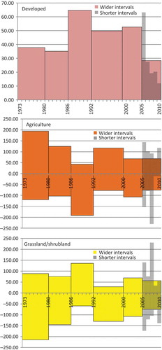
When summarizing overall change at the ecoregion level, the 2005–2010 interval returns a 0.4% average annual rate of change, lower than any of the annual estimates (which ranged between 0.5% and 1.1%). This rate is low because many of the areas that changed in each year between 2005 and 2010 were areas that converted multiple times and often returned to the same LULC class as the initial 2005 LULC class (such as fields that went out of production and returned to production in a 5 year window). When annual change is accounted for each year between 2005 and 2010, the overall change footprint in the Central California Valley ecoregion totaled 3.8%, or 1800 km², of the region. Using an interval-based approach for 2005–2010 greatly reduces the overall change footprint to 2.2%, or roughly 1000 km². The LULCC rate for the 2005–2010 interval (at 2.8% of the ecoregion, or nearly 1300 km²) was slightly lower than the overall change rate estimated for the new 2000–2005 interval.

Change by class describes the differences between the 2000–2005 and 2005–2010 intervals more thoroughly than overall spatial footprint change estimates. For example, net increases in development totaled 250 km² for 2000–2005, but only 140 km² for 2005–2010. Analysis of changes in development in the 2005–2010 interval gives the impression that development began to slow in 2005 and change rates were even lower than in the two intervals spanning 1973–1980 and 1980–1986. Yet, annual updates provide a more precise estimate of new development, with the onset of slowed development starting in 2006–2007 preceded by near historic highs in 2005–2006. Annual rates of new development between 2006 and 2010 were lower than any other time since 1973.

Agriculture declined in each of the two new intervals (2000–2005 and 2005–2010), but the 200 km² reduction for 2000–2005 was substantially larger than the 40 km² drop for 2005–2010. Similarly, grassland/shrubland showed a net decline of 190 km² between 2000 and 2005, yet only 90 km² between 2005 and 2010. Examination of LULCC using the 2005–2010 interval alone masks out significant interannual variability in LULCC. While the 2005–2010 interval shows a stable agriculture trend, annual LULCC analysis reveals net losses of 139 km² of agriculture between 2007 and 2008, losses completely undetectable in the interval. This single-year loss in agriculture was coupled with a 124 km² grassland/shrubland expansion between 2007 and 2008, also undetectable in the 2005–2010 interval, appearing as part of a continued grassland decline.

The wetland class has similar net increases in each interval, from 60 km² for 2000–2005 to 80 km² for 2005–2010. The only class that underwent a notable increase in one interval and a decrease in the following interval was nonmechanical disturbance. In this instance, small fires occurred in five of the 48 sample blocks in 2005, and vegetation reestablished by 2010. These fires led to a 71 km² increase in nonmechanical disturbance for 2000–2005, and an 84 km² decrease for 2005–2010 attributed to post-fire succession.

3.3. Long-term LULCC (1973–2010)

We combined our estimates with existing historical estimates to create a 37 year temporal window for analysis. Over the period 1973–2010, we estimate that 15.1% (or 6900 km²) of the Central California Valley ecoregion underwent at least one (Table 5). Of the 6900 km² that changed, 69% (or 4700 km²) of this area changed once and 31% (2200. km²) changed more than once. Approximately 800 km² of land changed three or more times.

Table 5. Footprint of change (percent of ecoregion) for 1973–2010 describes the percent of the Central California Valley ecoregion that underwent change in at least one of the intervals. Confidence interval (85%), standard error, and relative error of estimated change are also reported

Foot print	Ecoregion (%)	85% +/–	Standard error (%)	Relative error (%)
All change	15.1	3.3	2.3	15.1
1 Change	10.3	2.0	1.4	13.0
2 Change	3.1	1.2	0.8	27.0
3+ Changes	1.7	0.8	0.6	34.0

Average annual change rates were calculated from interval-based change estimates for the extended 37 year study period and reveal relatively consistent LULCC through time, highlighted by two periods of higher than average change. The 1973–1980 interval had an exceptionally high average annual rate of change and was marked as the period with the greatest amount of grassland/shrubland to agriculture land conversions. Over this period, roughly 360 km² of land changed annually (Sleeter, 2008). The four intervals extending through 2005 (1980–1986, 1986–1992, 1992–2000, 2000–2005) had similar average annual change rates, ranging from 230 to 280 km² of change per year.

Despite fluctuations between temporal intervals, agriculture in 2010 had only decreased by 0.5% (160 km²) in total area compared to 1973. Grassland/shrubland fluctuated substantially, declining by 22% (1930. km²) by 2010. Roughly one-seventh of these losses occurred from 2000 to 2010. Most of the losses in grasslands/shrublands were the result of gains in agriculture and development. The development footprint increased by 55% between 1973 and 2010 (1650. km²), and 9.3% between 2000 and 2010 (400 km²). Finally, the wetland footprint increased by 48%, or 320 km², between 1973 and 2010. The 17% increase (140 km²) in wetlands since 2000 shows that wetland growth has remained substantial even in recent years.

LULC classes like agriculture, water, and wetlands tend to fluctuate along with variations in climate conditions and water availability. The leading LULC conversion for the period 1973–2010 was grassland/shrubland to agriculture which totaled 2400 km². Most of the gains in agriculture from grasslands/shrublands occurred in the 1973–1980 interval, when roughly half of these conversions took place. A small proportion of grassland/shrubland to agriculture conversions occurred in the last 10 years of the 37 year study period.

The top conversions estimated between 2000 and 2010 were similar to the top changes mapped over the extended study period (1973–2010): LULC conversions from agriculture and grassland/shrubland to development remain major conversions in each temporal interval. Between 2000 and 2010, we estimated that 400 km² in new development was constructed in the Central California Valley ecoregion. Conversions to new development for 2000–2005 (51 km²/year) and 2005–2006 (63 km²/year) kept pace with historical development rate estimates from 1986 to 1992 (65 km²/year) and from 1992 to 2000 (49 km²/year) (Sleeter, 2008). According to our estimates, conversions to developed lands began to slow between 2006 and 2007 (27 km²/year). Slowing development rates continued through 2009–2010, when only 12 km² of new development was estimated for the entire ecoregion. The rate of development for each year between 2006 and 2010 was lower than any other time in the LULCC record.

Several LULCC differences appear between the late twentieth century and early twenty first century estimates. Losses of agriculture to grasslands/shrublands and wetlands show shifting trends in modern LULC. Most of the gains in wetlands occurred in the 6 year 1980–1986 interval (79 km² net increase), but conversions to wetlands in 2000–2005 (61 km² net increase) and 2006–2007 (66 km² net increase) resulted in higher than average conversions to wetlands in the last 10 years of the extended study period. Changes from agriculture to grasslands/shrublands increased in drought years, and were most pronounced in 1986–1992 (131 km² converted annually) during an extended drought period (Sleeter, 2008), but also substantial during 2007–2008 amidst a shorter drought (208 km² converted annually). Collectively, higher than average losses of agriculture to grassland/shrublands in 2000–2005 (66 km² converted annually), in conjunction with drought-related losses in 2007–2008, resulted in above average conversions for 2000–2010. In most cases, areas that lost agriculture to grassland/shrubland cover eventually resumed agricultural production once water availability increased or a crop shift took place.

4. Discussion

Water availability is the key limiting factor to agricultural production in the Central California Valley ecoregion. The Sacramento River, California’s largest drainage basin, is the principal source of irrigated water for farmers in both the Sacramento and San Joaquin Valleys. Nearly 75% of the state’s water demand comes from the south, while nearly 75% of the precipitation falls in the north. Much of the water from the Sacramento River is diverted south of its natural drainage into the San Francisco Bay Delta by the Central Valley Project (CVP), a federal program administered by the US Bureau of Reclamation. This water is pumped into the Delta Mendota Canal at the Tracy Pumping Station (also referred to as the C.W. Bill Jones Pumping Station) for deliveries to the San Joaquin Valley, south of the Delta. The semiarid San Joaquin Valley receives only 25% of the precipitation and 25% of the total Central Valley runoff compared to the north (California Department of Water Resources, 2011), yet produces half of California’s agriculture output. With such heavy reliance on nonlocal sources of irrigation water, interannual fluctuations in precipitation and subsequent runoff can have significant impacts on water availability for farmers. Additionally, changes in water policy can also have adverse impacts on regional agriculture.

To look at the overall effect of regional climate and drought conditions on agriculture, we compiled late-winter (January to March) average monthly Palmer Drought Severity Index (PDSI) values for the California Climate Division 2 (Sacramento drainage) and Division 5 (San Joaquin drainage). PDSI measures relative dryness or wetness using monthly temperature and precipitation to create conditional categories. Positive PDSI values indicate wet conditions and negative values indicate dry conditions (National Oceanic and Atmospheric Administration, 2011). We also compiled basin-wide runoff data for both the Sacramento and San Joaquin River basins (California Department of Water Resources, 2011) and monthly total pumping data from the C.W. Bill Jones Pumping Station (U.S. Bureau of Reclamation, 2012). Finally, we compared LULC estimates from our study to biennial agricultural change reports released by the Farmland Mapping and Monitoring Program (FMMP) for the period 2000–2008 (California Department of Conservation, 2010), California Farmland Conversion Reports (California Department of Conservation, 2011), and county crop reports for the 2009 crop year (Madera County, 2010; Tulare County, 2010).

Figure 4 depicts annual runoff, PDSI, CVP water allocations, and net change in agriculture land use in the Central California Valley from 1973 to 2010. Annual water year runoff closely follows average late-winter (January through March) PDSI values (Figure 4). Late-winter PDSI values were selected as an indicator of overall future snowmelt and spring runoff potential, given California’s winter-dominant precipitation regime. During the 1987–1992 drought (negative PDSI), water allocations did not decline until 3 years into the drought, likely a result of the series of preceding wet years (1982., 1983, 1984, and 1986) that filled reservoirs and enabled continued contractual water deliveries (California Department of Water Resources, 2012). Statewide reservoir storage did not achieve severe drought classification for two consecutive months until March of 1990 when water allocations concurrently declined 50% (California Department of Water Resources, 2012). Interval estimates of net agriculture land-use change track overall PDSI trends; however, the 1987–1992 drought signal would likely have been missed if the temporal interval had concluded in 1993. Comparing late-winter PDSI and CVP water allocations with net changes in agriculture lands reveals the close link between water availability and fluctuations in agriculture extent (Figure 4). When allocations drop below 100%, LULC estimates of agriculture also decline. Interval-based estimates in the early LULC record capture the overall trend, yet the modern annual LULC estimates show a 1 year lag time between net agriculture change and water allocation.

Figure 4. Top panel represents annual water year (October through September) discharge from the Sacramento Valley (dark shaded area) and San Joaquin Valley (light shaded) measured as un-impaired runoff in millions of acre feet (California Department of Water Resources, 2011), along with values for the Palmer Drought Severity Index (black line). The middle panel shows Central Valley Project (CVP) water allocations to agricultural contractors from 1977 to 2010 expressed as a percent of total contract amount delivered and the bottom panel shows net change in agriculture in +/– square kilometers found in this study. The two vertical lines are included to show agreement between data during drought.

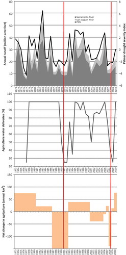
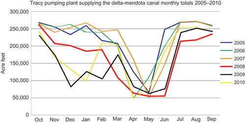
The annual net agriculture change estimates (2005–2010) show a 1 year lag response to developing drought conditions, culminating in a marked decline in agriculture land use in 2008. Runoff totals in both the Sacramento and San Joaquin Valleys in 2008 were classified as ‘critical’, a designation worse than drought (California Department of Water Resources, 2011). Low inflow coupled with the federally mandated flow restrictions put in place in December 2007 to protect the Delta smelt (Hypomesus transpacificus) fish species also diminished total allowable water exports from the Bay Delta in 2008 (Natural Resources Defense Council & et al. v. Kempthorne, 2007). Monthly data from 2005 to 2010 from the Tracy Pumping Plant show that the lowest rates of pumping occurred from late spring through September 2008 (Figure 5). In 2008, our estimates capture the single greatest drought-induced decline in agriculture since the 1987–1992 drought captured in the interval analysis (Figure 4).

Figure 5. Monthly total pumping at the Tracy Pumping Plant in acre feet for water years (October – September) 2005 through 2010.

We estimated a small net increase in agriculture in 2009, a drought year in the Sacramento drainage, but only below normal for the San Joaquin drainage (Figure 4). CVP water allocations were at only 25% in 2009, nearly 15% lower than in 2008. Water shortages in 2009 coincide with formal declarations, at the national and state levels, regarding California’s drought emergency (California Department of Water Resources, 2010). The small increase in runoff, relative to the 2 years prior, may have contributed to the small increase in the agricultural footprint found in our research. Some studies (California Department of Water Resources, 2010; Cody, Folger, & Brougher, 2009) also suggest that litigation intermittently halting water pumping across the Central California Valley had a negative impact on crop production, forcing many farmers across the region to rely on increased groundwater pumping to offset drought conditions (Faunt, 2009). Closer examination reveals net agriculture increases in 2009 that occurred primarily in Madera, Merced, and Kern Counties, may likely be attributed to increased groundwater pumping. Groundwater has often been used to offset reductions in surface water access (Faunt, 2009). While groundwater has a history of sustaining crop yields through difficult times, it quickly becomes overdrafted in the Central California Valley during drought years (Faunt, 2009). Satellite analysis shows the average groundwater depletion rate doubling between 2006 and 2010 to offset reduced surface water pumping (Famiglietti et al., 2011). The stabilization of agriculture found in our 2009 estimates may also be partly explained by the increase in surface pumping, starting in early March 2009 (Figure 5), following February where precipitation was 160% of average (Zhang et al., 2003). This anomalously wet month, along with higher overall pumping relative to 2008, contributed to reservoir storage levels in the south at over 80% the historical average (California Department of Water Resources, 2010), and may have ultimately provided farmers with some relief following formal declarations of drought emergencies at the beginning of 2009 (Cody et al., 2009).

Annual crop reports also reflect how drought and water deliveries impact cropping practices and spatial redistributions across the Central California Valley. At the state level, agricultural losses between 2007 and 2008 occurred in water-intensive cotton and rice, as well as all livestock, vegetable, and melon crops (California Department of Conservation, 2011, USDA National Agricultural Statistics Service, 2011). Dryland and orchard farming (almonds, pistachios, and olives) increased at this time, offsetting total irrigated crop losses. In select counties, irrigated pasture and field crops underwent losses in production (tons), while the rate of expansion in orchard production merely slowed relative to recent trends. Although our results are not spatially explicit, the random samples that contributed to the decline in agriculture in 2008 were located in Tulare and Madera Counties where beans, cotton, other field crops, and irrigated pasture declined (Madera County, 2010; Tulare County, 2010). County crop reports generally show a continued decline of agriculture for 2007–2009, but these reports also identify growth in select crop types between 2008 and 2009. In 2009, fruit and nut trees continued to expand production, while some vegetable and melon crops rebounded from 2008 levels. In our sample blocks, most of the gains for 2008–2009 (69 km² valley wide) occurred in Madera County, which underwent an increase in pasture and nut crops in 2009. The mapped installation of center pivot irrigation in 2009, along with Madera County crop data, suggests that the expansion occurred in high-value vegetable crops (Madera County, 2010). Additionally, the use of center pivot may also be a sign of more groundwater use, which increased statewide during the drought years of 2007–2009 to offset lower irrigation water deliveries (Famiglietti et al., 2011).

Our annual estimates of agriculture and urban change are similar to estimates reported by FMMP for the period 2000–2008 (California Department of Conservation, 2010), providing additional insight into why certain land-cover changes have taken place in recent years. Between 2002 and 2008, the amount of irrigated farmland decreased dramatically (2000. km² lost) at over 3.5 times the rate of the 1996–2002 period (550 km² lost). Areas categorized as ‘prime farmland’ for having the highest-quality soils were also heavily impacted, with total losses more than doubling in 2002–2008 relative to the 1996–2002 period. FMMP cites environmental factors such as salinity, drought, and socioeconomic stressors as contributing to overall loss of farmland, yet these conditions have led to the replacement of water-intensive crops with high-value perennial crops (e.g., almond and pistachio orchards) and dairy farms. The recent trend toward high-value crops has also been reported elsewhere (Blake, 2009). According to FMMP, some of the agricultural losses can be attributed to urban growth, while most were reflected as conversions to idle land. Some former agricultural lands even gradually converted back to wetlands, driven by wetland reserve easements and wildlife refuge additions (California Department of Conservation, 2010). These conversions match the recent growth in wetlands found in our research.

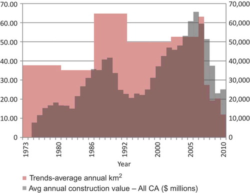
The low-intensity development into agricultural lands cited by FMMP also supports our findings, increasing steadily through 2006 before slowing significantly during 2006–2008 (California Department of Conservation, 2010). The near 43% decline in the rate of new development in 2006–2007 and continued decline each year correspond with the 2007 onset of the global financial crisis, commonly referred to as the Great Recession. This crisis, characterized by subprime mortgages, the loss of over 1 million jobs, and a 23% decline in exports across California, marked the beginning of unprecedented foreclosure rates which peaked in 2008 and still plague the region today (RAND California, 2010; Bardhan & Walker, 2011). The Central Valley is currently home to 5 of the top 10 foreclosure cities in the country, with Modesto (#2), Stockton (#4), Sacramento (#6), Bakersfield (#7), and Fresno (#8), all making the list (Aalbers, 2009; RealtyTrac, 2011). Statewide, these factors contributed to the construction of new residential buildings declining by over 400% between 2005 and 2008 (California Department of Finance, 2012). California Department of Finance (CDOF) data record statewide construction expenditures and show good concordance with the annual estimates of new developed land and the declines in new development coinciding with the Great Recession (Figure 6). CDOF data track overall trends in development over the entire LULC record, yet shows the strongest relationship with the annual estimates of developed LULC, highlighting the importance of economic indicators as drivers of LULCC.

Figure 6. Comparison between annualized estimates of new development and statewide annual construction values compiled by the California Department of Finance (2012).

5. Conclusion

Within the Central California Valley ecoregion, 2000–2010 LULCC has been largely characterized by annual shifts in agriculture production, slowing development rates, and declining grassland/shrubland cover. Agricultural fluctuations are primarily driven by climate dependency and shifts in water allocation rights within the region’s highly engineered water delivery system. Losses of historically prime farmland and grassland/shrubland to rural and urban development have also become a growing concern, despite occurring at a slower rate in recent years due to economic instability. Given the widespread availability of daily-to-annual biogeophysical (e.g., climate station data, stream gage data, air quality measurements) and anthropogenic (e.g., water pumping data, cropland data, construction rates) data sets, the results described here not only demonstrate how annual change estimates can be more effectively linked to regional change drivers, but also provide more detailed change information than interval-based approaches regarding the duration of drivers operating over short time periods. For instance, LULCC resulting from the 2007–2009 drought or Great Recession would have been masked or subdued using a wider interval (2005–2010) compared to annual mapping.

The method applied here to estimate LULCC in the Central California Valley for 2000–2010, while leveraging a previous change detection effort for 1973–2000 (Sleeter, 2008), also serves as an effective way to extend prior monitoring efforts and examine longer-term trends. The 1973–2010 data reported here represent the most comprehensive story of LULCC for the Central California Valley to date. Even though the long-term trend in agricultural extent was generally flat, fluctuations that did occur exhibited sensitivity to drought or policy-driven changes in water availability. Development increased overall, despite slowing in recent years due to economic instability.

Even in times where driving forces serve to slow land change, humans continue to alter the landscape. As anthropogenic land-use change persists into the future, additional pressure will be placed on already limited land and water resources. Developed land uses are projected to continue to expand into prime farmlands and place additional burden on available water (California Department of Water Resources, 2009). Policies such as the Williamson Act may serve to slow development in the future, but no current policy has provided enough of an economic opportunity or constraint to stop development altogether (Goodenough, 1992). Given the amount of suitable agricultural land in the region, expansion of agriculture may continue to spill over into the adjacent Oak Woodlands ecoregion to accommodate demand (Sleeter, Wilson, Soulard, & Liu, 2011). Technological advances or intensified production may also lead to continued crop productivity; however, water availability will persist as the limiting factor in agriculture production. Given recent satellite observations measuring significant groundwater depletion in the Central California Valley, water resource use may have already reached unsustainable levels (Famigletti et al., 2011).

This study shows that an annual approach to long-term LULCC monitoring best captures anthropogenic LULCC and the feedbacks associated with such changes. This is especially true in areas with high rates of observed historic LULCC such as the Central California Valley. Producing annual LULCC estimates has many benefits over the temporal interval approach. Annualized LULCC estimates enable additional empirical analysis against other long-term records (e.g., climate station data, stream gage data, agricultural census data, water pumping, economic indicators) to determine impacts of change on the environment. Such estimates can also fine-tune baseline LULC in modeling efforts, providing more robust validation of future LULCC projections. Based on the methods described here, producing LULCC products annually rather than every 5 years may require as little as 20% additional investment of resources, particularly if post-classification methods are employed using existing LULC data sets as the baseline for change.

The development of continuous, long-term LULC records such as this can facilitate additional exploration into the consequences of landscape composition and change, enabling researchers to monitor linkages between LULC and biogeophysical processes across space and time. LULC composition and change has already been linked to water quality declines (Foley et al., 2005), climate change at regional and global scales (Bonan, 1997, Lawrence & Chase, 2010; Pielke et al., 1999, 2002; Pitman et al., 2011), carbon dioxide emissions (Houghton & Hackler, 2001), habitat loss (Seabloom, Dobson, & Stoms, 2002; Soule, 2001), species extinction (Davies et al., 2006), and declining air quality (Romero, Ihl, Rivera, Zalazar, & Azocar, 1999; Ross et al., 2006). Several national research programs are now tasked with understanding the interactions between LULC and LULCC and climate (e.g., US Geological Survey’s Climate and Land Use Change program, US Environmental Protection Agency’s Integrated Climate and Land Use Scenarios program). Monitoring the location and distribution of LULCC is also important for establishing links between policy decisions, regulatory actions, and land use (Hostert et al., 2011; Lunetta, Knight, Ediriwickrema, Lyon, & Worthy, 2006). Continuous LULCC monitoring allows researchers to draw connections between land change and variables such as carbon storage, watershed protection, and other ecosystem services – information essential for the management of natural and anthropogenic resources.

6. Acknowledgments

Updating the Central California Valley ecoregion through 2010 was supported by the USGS Land Change Science and USGS Climate and Land Use Change Research and Development programs. We would also like to thank William Acevedo and Benjamin Sleeter for their guidance, Dan Sorenson, Rachel Sleeter, and Amy Mathie for performing sample block interpretations, and Jeanne Jones for processing spatial statistics.

References

- Aalbers, M. (2009). Geographies of the financial crisis. Area Journal, 41(1), 34–42.
- Anderson, J. P., Hardy, E. E., Roach, J. T., & Witmer, R. E. (1976). A land use and land cover classification system for use with remote sensor data. U.S. Geological Survey Professional Paper, 964, 28.
- Bardhan, A., & Walker, R. (2011). California shrugged: Fountainhead of the great recession. Cambridge Journal of Regions, Economy and Society, 4(3), 303–322. doi:10.1093/cjres/rsr005.
- Blake, C. (2009). Central valley: Permanent crops, dairy increase; major cotton reduction. Saint Charles, IL: Western Farm Press. Retrieved from http://westernfarmpress.com/central-valley-permanent-crops-dairy-increase-major-cotton-reduction
- Bolliger, J., Wagner, H. H., & Turner, M. G. (2007). Identifying and quantifying landscape patterns in space and time. In F. Kienast, S. Ghosh, & O. Wildi ( Eds.), A changing world: Challenges for landscape research ( pp. 177–194). Dordrecht: Springer.
- Bonan, G. B. (1997). Effects of land use on the climate of the United States. Climatic Change, 37(3), 449–486.
- California Department of Conservation. (2010). Farmland mapping and monitoring program: Important farmland data availability. Retrieved from http://redirect.conservation.ca.gov/dlrp/fmmp/product_page.asp
- California Department of Conservation. (2011). California farmland conversion Report 2006–2008. Sacramento, CA: California Department of Conservation, Division of Land Resource Protection, Farmland Mapping and Monitoring Program. 108
- California Department of Finance. (2012). California construction data, annual data from 1975. Retrieved from http://www.dof.ca.gov/html/fs_data/latestecondata/FS_Construction.htm
- California Department of Water Resources. (2009). California water plan, Update 2009, Version 3, Sacramento, CA: Sacramento-San Joaquin River Delta. Retrieved from http://www.waterplan.water.ca.gov/docs/cwpu2009/0310final/v3_ssjdeltaregion_cwp2009.pdf
- California Department of Water Resources. (2010). California’s drought of 2007–2009: An overview. Sacramento, CA. Retrieved from http://www.water.ca.gov/waterconditions/drought/docs/DroughtReport2010.pdf
- California Department of Water Resources. (2011). Historical water supply indices, chronological reconstructed sacramento and San Joaquin valley water year hydrologic classification indices. Retrieved from http://cdec.water.ca.gov/cgi-progs/iodir/wsihist
- California Department of Water Resources. (2012). California reservoirs – drought status percentiles. California Data Exchange Center. Retrieved from http://cdec.water.ca.gov/cdecapp/drought/getres.action
- California Regional Water Quality Control Board. (2010). Groundwater quality protection strategy central valley region roadmap. Rancho Cordova, CA: California Regional Water Quality Control Board, Central Valley Region Control Board. 100.
- Cody, B., Folger, P., & Brougher, C. (2009). California drought: Hydrological and regulatory water supply issues. Congressional Research Service. Retrieved from http://www.fas.org/sgp/crs/misc/R40979.pdf
- Coppin, P., Jonckheere, I., Nackaerts, K., Muys, B., & Lambin, E. (2004). Digital change detection methods in ecosystem monitoring: A review. International Journal of Remote Sensing, 25(9), 1565–1596.
- Cousins, S. A. O. (2001). Analysis of land-cover transitions based on 17th and 18th century cadastral maps and aerial photographs. Landscape Ecology, 16, 41–54.
- Davies, R. G., Orme, D. L., Olson, V., Thomas, G. H., Ross, S. G., Ding, T.-S., . . . Gaston, K. J. (2006). Human impacts and the global distribution of extinction risk. Proceedings of the Royal Society Biological Sciences, 273, 2127–2133.
- Famiglietti, J. S., Lo, M. L., Ho, S. L., Bethune, J., Anderson, K. J., Syed, T. H., . . . Rodell, M. (2011). Satellites measure recent rates of groundwater depletion in California’s Central Valley. Geophysical Research Letters, 38, 4. doi:201110.1029/2010GL046442
- Faunt, C. C. ( Ed.) (2009). Groundwater Availability of the Central Valley Aquifer, California. U.S. Geological Survey Professional Paper 1766. Retrieved from http://pubs.usgs.gov/pp/1766/PP_1766.pdf
- Ferranto, S., Huntsinger, L., Getz, C., Nakamura, G., Stewart, W., Drill, S., . . . Kelly, M. (2011). Forest and rangeland owners value land for natural amenities and as financial investment. California Agriculture, 65(4), 184–191.
- Foley, J. A., DeFries, R., Asner, G. P., Barford, C., Bonan, G., Carpenter, S. R., . . . Snyder, P. K. (2005). Global Consequences of Land Use. Science, 309, 570–574.
- Fry, J., Xian, G., Jin, S., Dewitz, J., Homer, C., Yang, L., . . . Wickham, J. D. (2011). Completion of the 2006 national land cover database for the conterminous United States. Photogrammetric Engineering & Remote Sensing, 77(9), 858–864.
- Goodenough, R. (1992). Room to grow? Farmland conversion in California. Land Use Policy, 9(1), 21–35.
- Goward, S. N., Masek, J. G., William, D. L., Irons, J. R., & Thompson, R. J. (2001). The Landsat 7 mission: Terrestrial research and applications for the 21st century. Remote Sensing of Environment, 78(1–2), 3–12.
- Houghton, R. A., & Hackler, J. L. (2001). Carbon flux to the atmosphere from land-use changes: 1850 to 1990. ORNL/CDIAC-131, NDP-050/R1. Carbon Dioxide Information Analysis Center, U.S. Department of Energy, Oak Ridge National Laboratory, Oak Ridge, Tennessee, USA doi:10.3334/CDIAC/lue.ndp050
- Hostert, P., Kuemmerle, T., Prishchepov, A., Sieber, A., Lambin, E. F., & Radeloff, V. C. (2011). Rapid land use change after socio-economic disturbances: The collapse of the Soviet Union versus Chernobyl. Environmental Research Letters, 6(045201), 8. doi:10.1088/1748–9326/6/4/045201
- IPCC. (2007). Contribution of working group I to the fourth assessment report of the intergovernmental panel on climate change. In S. Solomon, D. Qin, M. Manning, Z. Chen, M. Marquis, K. B. Averyt, M. Tignor, & H. L. Miller ( Eds.), Climate change 2007: The physical science basis. Cambridge: Cambridge University Press.
- Lambin, E. F. (1996). Change detection at multiple temporal scales: Season and annual variations in landscape variables. Photogrammetric Engineering & Remote Sensing, 62(8), 931–938.
- Lambin, E. F., Turner, B. L., Geist, H. J., Agbola, S. B., Angelsen, A., Bruce, J. W., . . . Xu, J. (2001). The causes of land-use and land-cover change: Moving beyond the myths. Global Environmental Change, 11, 261–269.
- Lawrence, P. L., & Chase, T. N. (2010). Investigating the climate impacts of global land cover change in the community climate system model. International Journal of Climate, 30, 2066–2087.
- Lee, G. F., & Jones-Lee, A. (2002). Issues in developing a water quality monitoring program for evaluation of water quality – beneficial use impacts of stormwater runoff and irrigation water discharges from irrigated agriculture in the Central Valley, CA. (California Water Institute Report TP 02–07), Fresno, CA: California Water Resources Control Board and Central Valley Regional Water Quality Control Board, California State University Fresno, 157.
- Li, M., Huang, C., Zhu, Z., Shi, H., Lu, H., & Peng, S. (2009). Assessing rates of forest change and fragmentation in Alabama, USA, using the vegetation change tracker model. Forest Ecology & Management, 257, 1480–1488.
- Loveland, T. R., Sohl, T. L., Stehman, S. V., Gallant, A. L., Sayler, K. S., & Napton, D. E. (2002). A strategy for estimating the rates of recent Unites States land cover changes. Photogrammetric Engineering and Remote Sensing, 68(10), 1091–1099.
- Lunetta, R. S., Knight, J. F., Ediriwickrema, J., Lyon, J. G., & Worthy, L. D. (2006). Land cover change detection using multi-temporal MODIS NDVI data. Remote Sensing of Environment, 105, 142–154.
- Madera County. (2010). 2009 Agricultural crop report, Madera County Department of Agriculture. Retrieved from http://ucanr.org/sites/Farm_Management/files/132045.pdf
- Napton, D., Auch, R., Headley, R., & Taylor, J. (2010). Land changes and their driving forces in the Southeastern United States. Regional Environmental Change, 10, 37–53.
- National Oceanic and Atmospheric Administration. (2011). National climatic data center, California palmer drought severity index database. Retrieved from http://www.ncdc.noaa.gov/temp-and-precip/time-series/?parameter=pdsi&month=1&year=2004&filter=1&state=4&div=0
- Natural Resources Defense Council, et al. V. Kempthorne. (2007). Findings of fact and conclusions of law re. interim remedies re: Delta smelt esa remand and reconsultation, Eastern District of California: United States District Court, 1:05-cv-1207 OWW GSA.
- Omernik, J. M. (1987). Ecoregions of the conterminous United States. Annals of the Association of American Geographers, 77, 118–125.
- Phinn, S. R., Stow, D. A., Franklin, J., Mertes, L. A. K., & Michaelsen, J. (2003). Remotely sensed data for ecosystem analyses: Combining hierarchy theory and scene models. Environmental Management, 31(3), 429–441.
- Pielke, R. A., Marland, G., Betts, R. A., Chase, T. N., Eastman, J. L., Niles, J. O., . . . Running, S. W. (2002). The influence of land-use change and landscape dynamics on the climate system: Relevance to climate-change policy beyond the radiative effect of greenhouse gases. Philosophical Transactions of the Royal Society of London, 360, 1705–1719.
- Pielke, R. A., Walko, R. L., Steyaert, L. T., Vidale, P. L., Liston, G. E., Lyons, W. A., & Chase, T. N. (1999). The influence of anthropogenic landscape changes on weather in South Florida. Monthly Weather Review, 127, 1663–1672.
- Pitman, A. J., Avila, F. B., Abramowitz, G., Wang, Y. P., Phipps, S. J., & de Noblet-Ducoudre, N. (2011). Importance of background climate in determining the impact of land-cover change on regional climate. Nature Climate Change, 1, 472–475.
- RAND California. (2010). Housing foreclosures in California Counties and Cities [data file]. Retrieved from http://ca.rand.org/stats/economics/foreclose.html
- RealtyTrac. (2011). U.S. foreclosure activity increases 7 percent in August, defaults surge 33 percent. Retrieved from http://www.realtytrac.com/content/foreclosure-market-report/august-2011-us-foreclosure-market-report-6836
- Romero, H., Ihl, M., Rivera, A., Zalazar, P., & Azocar, P. (1999). Rapid urban growth, land-use changes and air pollution in Santiago, Chile. Atmospheric Environment, 33, 4039–4047.
- Ross, Z., English, P. B., Scalf, R., Gunier, R., Smorodinsky, S., Wall, S., . . . Jerrett, M. (2006). Nitrogen dioxide prediction in Southern California use land use regression modeling: Potential for environmental health analyses. Journal of Exposure Science and Environmental Epidemiology, 16, 106–114.
- Roy, D. P., Ju, J., Kline, K., Scaramuzza, P. L., Kovalskyy, V., Hansen, M. C., . . . Zhang, C. (2010). Web-enabled Landsat Data (WELD): Landsat ETM+ Composited mosaics of the conterminous United States. Remote Sensing of Environment, 114, 35–49.
- Seabloom, E. W., Dobson, A. P., & Stoms, D. M. (2002). Extinction rates under nonrandom patterns of habitat loss. Proceedings of the National Academy of Sciences, 99(17), 11229–11234.
- Sleeter, B. M. (2008). Late 20th century land change in the Central California Valley Ecoregion. The California Geographer, 48, 27–60.
- Sleeter, B. M., Wilson, T. S., Soulard, C. S., & Liu, J. (2011). Estimation of late Twentieth century land-cover change in California. Environmental Management and Assessment, 173, 251–266.
- Smits, P. C., & Annoni, A. (1999). Updating land-cover maps by using texture information from very high-resolution space-borne imagery. IEEE Transactions on Geoscience and Remote Sensing, 37(3), 1244–1254.
- Sohl, T. L., Loveland, T. R., Sleeter, B. M., Sayler, K. L., & Barnes, C. A. (2010). Addressing foundational elements of regional land-use change forecasting. Landscape Ecology, 25(2), 233–247.
- Soule, M. E. (2001). Conservation: Tactics for a constant crisis. Science, 253, 744–750.
- Stehman, S. V., Sohl, T. L., & Loveland, T. R. (2003). Statistical sampling to characterize recent United States land-cover change. Remote Sensing of Environment, 86(4), 517–529.
- Tulare County. (2010). 2009 Tulare County annual crop and livestock report, Tulare County Agricultural Commissioner. Retrieved from http://agcomm.co.tulare.ca.us/default/index.cfm/linkservid/A3199C8C-F1F6-BDD5-85375618222DDE21/showMeta/0/
- Turner, M. G. (2005). Landscape ecology: What is the state of the science? Annual Review of Ecology, Evolution and Systematics, 36, 319–344.
- Turner, M. G., Gardner, R. H., & O’Neill, R. V. (2001). Landscape ecology in theory and practice: Pattern and process. New York, NY: Springer. 424.
- U.S. Bureau of Reclamation. (2012). Jones (Tracy) pumping – historical data. Sacramento, CA: U.S. Bureau of Reclamation, Mid-Pacific Region, Central Valley Office. Retrieved from http://www.usbr.gov/mp/cvo/vungvari/tracy_pump.pdf
- U.S. Census Bureau. (2011). Population distribution and change: 2000 to 2010. Retrieved from http://www.census.gov/prod/cen2010/briefs/c2010br-01.pdf
- USDA National Agricultural Statistics Service. (2011). California historical data. Retrieved from http://www.nass.usda.gov/Statistics_by_State/California/Publications/index.asp
- U.S. Environmental Protection Agency. (1999). Level III ecoregions of the continental United States [digital map]. Corvallis, OR: U.S. Environmental Protection Agency, National Health and Environmental Effects Research Laboratory, scale 1:250,000.
- U.S. Geological Survey. (2007). Facing tomorrow’s challenges—U.S. Geological Survey science in the decade 2007–2017: U.S. Geological Survey Circular 1309. Retrieved from http://pubs.usgs.gov/circ/2007/1309/
- Western Regional Climate Center. (2012). California climate tracker. Desert Research Institute. Retrieved from http://www.wrcc.dri.edu/monitor/cal-mon/index.html
- Zhang, X., Friedl, M. A., Schaaf, C. B., Strahler, A. H., Hodges, J., Gao, F., . . . Huete, A. (2003). Monitoring vegetation phenology using MODIS. Remote Sensing of Environment, 84(3), 471–475.