Modeled historical land use and land cover for the conterminous United States

ABSTRACT

The landscape of the conterminous United States has changed dramatically over the last 200 years, with agricultural land use, urban expansion, forestry, and other anthropogenic activities altering land cover across vast swaths of the country. While land use and land cover (LULC) models have been developed to model potential future LULC change, few efforts have focused on recreating historical landscapes. Researchers at the US Geological Survey have used a wide range of historical data sources and a spatially explicit modeling framework to model spatially explicit historical LULC change in the conterminous United States from 1992 back to 1938. Annual LULC maps were produced at 250-m resolution, with 14 LULC classes. Assessment of model results showed good agreement with trends and spatial patterns in historical data sources such as the Census of Agriculture and historical housing density data, although comparison with historical data is complicated by definitional and methodological differences. The completion of this dataset allows researchers to assess historical LULC impacts on a range of ecological processes.

KEYWORDS:

• Land cover
• land use
• historical
• modeling
• United States
• FORE-SCE

1. Introduction

Land use and land cover (LULC) in the United States (US) has changed dramatically in the last few centuries. Land use and land management have directly changed the landscape through land use conversion, or have indirectly changed the landscape by altering successional and disturbance regimes. Half or more of the historical forest extent in the eastern US has been cleared in the last three centuries, with forest area rebounding during the twentieth century as agricultural activities shifted westward (Clawson, 1979; Drummond & Loveland, 2008). The expansion of agriculture in the Midwest and Great Plains has nearly eliminated native tallgrass prairie and severely reduced mixed- and short-grass prairies (Askins et al., 2007; Samson, Knopf, & Ostlie, 2004). In both the western and the southeastern US, forests managed as crops have replaced many natural forests (Birdsey, Pregitzer, & Lucier, 2006; Brown, Johnson, Loveland, & Theobald, 2005), while across the US urban growth has permanently altered the landscape. With a changing landscape, natural processes have been forever altered, with climate (Chase, Pielke, Kittel, Nemani, & Running, 2000; Pielke et al., 2011), carbon (Tian et al., 2012; Zhao, Liu, Sohl, Young, & Werner, 2013), hydrology (Frans, Istanbulluoglu, Mishra, Munoz-Arriola, & Lettenmaier, 2013; Yang et al., 2015), and biodiversity (Wilcove, Rothstein, Dubow, Phillips, & Losos, 1998) impacted by LULC change. An understanding of historical LULC is needed to understand the past effects of LULC change on ecological and societal processes, and to facilitate the modeling of potential future LULC change to support planning and mitigation efforts (Ramankutty & Foley, 1999; Trueman, Hobbs, & Van Niel, 2013).

Multiple contemporary, spatially explicit LULC databases are available for the conterminous US at moderate spatial and thematic resolutions, including the National Land Cover Database (NLCD) (Fry et al., 2011; Vogelmann et al., 2001), Landscape Fire and Resource Management Planning Tools Project (LANDFIRE) (Rollins, 2009), and the US Geological Survey (USGS) Land Cover Trends project (referred to as the ‘Trends’ project for the remainder of the article) (Loveland et al., 2002; Sleeter et al., 2013). However, spatially explicit, national-scale LULC data available for the US are based on remote sensing data, and as such, are limited to the historical lifespan of satellite systems and their sensors. While modeling is often used to produce future landscape projections, the modeling and reconstruction of historical landscapes are relatively rare (Ray & Pijanowski, 2010). The historical modeling that has been done has typically been spatially coarse, covered a small geographic area, and/or has been thematically simple (often just one LULC class such as crop or urban). For example, Hurtt et al. (2011) produced historic and projected, fractional LULC for the globe from 1500 to 2100, but at a coarse 0.5 degree resolution and for a limited number of land use classes. Ramankutty and Foley (1999) modeled at a higher resolution (0.5 minute) from 1992 back to 1700 for the globe, but only modeled one class (croplands). Zumkehr and Campbell (2013) produced gridded maps from 1850 to 2000, but also only modeled croplands. Fuchs, Herold, Verburg, Clevers, and Eberle (2014) modeled 5 LULC classes back to 1900 at a 1-km resolution, but for Europe, with no coverage for the US. Steyaert and Knox (2008) produced thematically detailed historical LULC for the eastern US, but the data were spatially and temporally coarse (20-km grid cells, with four individual maps for 1650, 1850, 1920, and 1992). Multiclass, moderate- to high-resolution historical data that have been modeled for the US tend to cover small geographic areas, such as the work of Ray and Pijanowski (2010) who modeled seven LULC classes for a small watershed in Michigan. The most thematically and spatially detailed historical LULC maps available for the conterminous US were recently produced by Falcone (2015), but these five maps (1974, 1982, 1992, 2002, and 2012) are heavily focused on anthropogenic land use, and still do not extend to dates prior to the Landsat era (i.e., prior to 1972).

Efforts to consistently and repeatedly map LULC at a national scale for the US did not begin until the 1992 NLCD (Vogelmann et al., 2001), but recent modeling work has attempted to ‘temporally extend’ these data into the future. A LULC database (annual maps, 250-m resolution, 16 LULC classes similar to NLCD) was created for the conterminous US for the years 1992–2100, with four unique scenarios for the years 2006–2100 (Sleeter et al., 2012; Sohl et al., 2014, 2012). The goal of this current work was to use a land cover modeling framework to extend the existing 1992–2100 database backwards in time, for dates prior to the availability of broad-scale remote-sensing data. This article describes:

1. A methodology developed to use a variety of historical data sources to model spatially explicit LULC from 1992 back to 1938;

2. An assessment of model results, including a quantitative and spatial comparison to existing historical data sources, and;

3. A discussion of the characteristics and use of the data caveats to this approach, and future research directions.

2. Methods

Modeling focused on the use of well-quantified historical data sources on anthropogenic land use change to actively quantify and model cropland, pasture, urban area, and reservoirs. Overlapping historical datasets provided historical, quantitative area for these classes at a regional level (e.g., county, ecoregion, or state), enabling us to directly model changes in these classes. Similarly, quantitative information on wetland change was available at a regional level, enabling direct parameterization and modeling There was far less quantitative and spatial data on historical extent of most ‘natural’ land covers (e.g., forest, grassland, shrubland). These classes were thus passively modeled, with quantitative and locational change in these classes resulting from modeled changes in the actively modeled classes. The selected modeling period from 1938 to 1992 reflects 1) a desired historical data period from partner institutions, 2) availability of historical data (with our starting date corresponding to a reporting date from the Agricultural Census), and 3) the need to ensure a consistent, seamless timeline with the aforementioned 1992–2100 USGS LULC data. The Forecasting Scenarios of Land use Change (FORE-SCE) model (Sohl et al., 2014; Sohl, Sayler, Drummond, & Loveland, 2007; Sohl et al., 2012) was used to produce the historical backcasts. FORE-SCE uses a modular approach with the demand component specifying overall, regional-level proportions of landscape change over time, while the spatial allocation component uses demand as a prescription and produces spatially explicit LULC maps based on suitability surfaces that quantify the ability of a given location to support each modeled LULC class.

Historical remote sensing databases were combined with a variety of other historical data sources to construct historical demand for the same LULC classes modeled as part of the Sohl et al. (2014) 1992–2100 database. Modeling for a historical period allowed for the direct use of historical census and remote sensing-based data sources, but the incorporation of these historical data is often not straightforward (Ray & Pijanowski, 2010; Verburg, Neumann, & Nol, 2011). Historical data come in a variety of formats and spatial scales, from spatially explicit raster and vector data, to spatially aggregated data such as county, state, or national estimates. Differences in thematic definitions of LULC further complicate the use of historical data (Herold, Mayaux, Woodcock, Baccini, & Schmullius, 2008). The following provides an overview of input data sources, issues related to discrepancies between input data, a description of the modeling framework, and the methods used to assess the final historical database.

2.1. Land cover data sources and spatial framework of the assessment

Modeling began with 1992 and proceeded backwards to 1938. The initial LULC data were a modified version of the 1992 NLCD (resampled to 250 m) that served as the initial data for the 1992–2100 LULC database (Sohl et al., 2014). Modeled LULC classes in this assessment include all classes within the 1992 NLCD, with the exception of NLCD’s multiple urban classes, which have been condensed into a single urban class. The classification scheme matches that from the 1992–2100 database, with the exception of forest cutting classes (as discussed below) (Table 1).

Table 1. Modeled LULC classes, and net change in LULC classes between 1938 and 1992 for the conterminous US. Values represent 1000s km².

Modeled LULC Proportions (1000s km^2)							1938 to 1992
	1938	1948	1958	1968	1978	1992
Water	181.6	193.9	205.7	214.7	220.3	227.8	+46.2 (+25.4%)
Urban	72.3	86.5	105.7	124.3	148.8	171.9	+99.7 (+137.9%)
Mining	4.6	4.6	4.8	5.0	5.6	6.7	+2.0 (+43.5%)
Barren	110.1	110.1	110.1	110.1	110.2	110.3	+0.2 (+0.2%)
Deciduous Forest	818.5	866.9	913.2	917.7	921.8	938.3	+119.8 (+14.6%)
Evergreen Forest	1,022.4	1,034.3	1,045.6	1,040.0	1,037.2	1,040.1	+17.7 (+1.7%)
Mixed Forest	288.9	309.0	330.6	335.4	338.5	347.8	+58.9 (+20.4%)
Grassland	1,185.3	1,260.9	1,258.5	1,218.7	1,239.2	1,240.1	+54.8 (+4.6%)
Shrubland	1,415.2	1,422.2	1.418.9	1.412.1	1.413.7	1.415.3	+0.1 (+0.0%)
Cropland	1,629.4	1,473.3	1,386.0	1,437.3	1,391.7	1,339.1	−290.2 (−17.8%)
Hay/Pasture	746.6	753.1	761.6	732.4	728.1	723.1	−23.5 (−3.1%)
Herb. Wetland	123.8	113.4	105.9	103.2	100.8	98.4	−25.5 (−20.6%)
Woody Wetland	281.1	251.5	233.3	228.7	223.9	220.9	−60.2 (−21.4%)
Ice/Snow	1.5	1.5	1.5	1.5	1.5	1.5	0.0

Historical LULC change from the Trends project (Loveland et al., 2002; Sleeter et al., 2013) was used in the reconstruction of historical LULC proportions (demand), and to parameterize the spatial allocation component of FORE-SCE. Trends used 10-km or 20-km sample blocks (typically 9–12 sample blocks for the 9 ecoregions that used 10-km blocks, or 25–40 sample blocks for the 75 ecoregions that used 20-km blocks) to estimate historical LULC change for each of 84 US Environmental Protection Agency (EPA) Level III ecoregions (U.S. EPA 1999) in the conterminous US Manual interpretation (a human interpreter visually digitizing LULC from underlying imagery) was used to create highly accurate LULC maps for 1973, 1980, 1986, and 1992, with change estimates for each ecoregion and time interval. The sample-based Trends data are suitable for quantifying overall rates of change at broad ecoregion scales (supplying demand), but do not provide spatially explicit LULC information across the entire conterminous US.

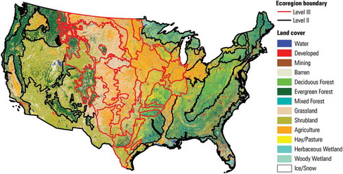
Level III and Level II ecoregions also served as the primary spatial framework for this modeling application. For the (eventually) mosaicked conterminous US LULC data, 27 ecoregions were modeled at the Level III ecoregion scale (nearly all in the Great Plains and the midwestern US), while the western US and eastern US were modeled at the Level II ecoregion scale. The difference in analysis scale reflects a change in available project resources that occurred after the Great Plains and Midwest were modeled. Both demand and the spatial allocation of change were parameterized individually for each ecological unit depicted in Figure 1. Implications of modeling the central US at the Level III ecoregion scale and the rest of the US at the Level II ecoregion scale are provided in the discussion section.

Figure 1. Ecoregions used as the spatial framework for modeling. In the Great Plains and upper Midwest, models were parameterized and run for each Level III ecoregion (27 ecoregions in total). Due to a reduction in resources, models were parameterized and run at the Level II ecoregion scale in the western and eastern US. The base land cover in the figure is the modified 1992 NLCD.

2.2. Construction of demand

FORE-SCE can use either simple proportions of future or historical LULC as demand, or can use a complete change matrix. For this work, we constructed a complete change matrix for each annual iteration of the model from 1992 back to 1938 for each ecoregion. A number of historical data sources were used to recreate historical change matrices but a sizeable challenge was harmonizing datasets with different spatial and thematic resolutions. Different historical datasets often also provide conflicting information on both the rates and types of historical LULC (Herold et al., 2008; Verburg et al., 2011). Given there can be substantial differences in even initial LULC class proportions between the starting 1992 NLCD and the data sources used to create historical demand, we used percentage change values from historical data sources but applied them to our starting 1992 NLCD quantities to determine the total amount of LULC change for each period. For example, if a historical reference source estimated a 5% decline in agricultural land going back in time, that 5% value was applied to our starting 1992 NLCD to determine demand.

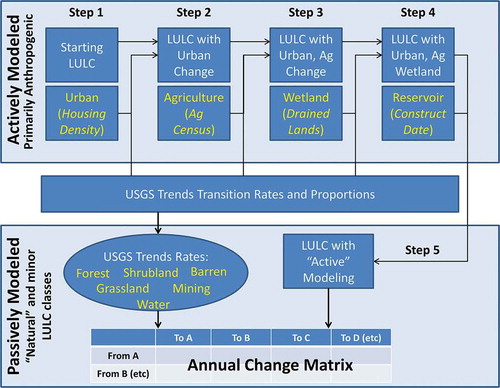
Given the lack of quantified historical data for most natural land covers, historical changes due to vegetation succession were omitted (e.g., natural succession between various forest classes). The effects of altered fire regimes and invasive species were also omitted due to a lack of consistent, national-scale historical information. A hierarchical approach was used in the construction of demand for each ecoregion, focusing on quantifying anthropogenic land use change at a regional scale, with natural land cover class proportions resulting from changes in anthropogenic land use (see Figure 2). The hierarchical approach begins with the quantification of historical demand for the urban class and agricultural classes (cropland and hay/pasture). Historic urbanized area was determined individually for each ecoregion from both Trends data and housing density data (Figure 2 – Step 1). Annual rates of urban change from 1992 back to 1973 were extracted from the Trends estimates, and applied to the amount of urban land in each ecoregion in 1992 to determine urbanized demand change. Regional rates of change from 1972 back to 1938 were determined from housing density data from Radeloff, Hagen, Voss, Field, and Mladenoff (2000).

Figure 2. Flowchart depicting Demand construction methodology. Demand construction begins with quantifying the ‘actively modeled’ classes of urban, agriculture (cropland and hay/pasture), wetland, and reservoirs. Quantity (net change) is determined using historical data layers represented in yellow, with USGS Land Cover Trends data used to determine the most likely LULC transitions to achieve net change. The quantity of ‘passively modeled’ classes (primarily natural LULC classes) result from transitions involving the (primarily anthropogenic) actively modeled classes, with USGS Land Cover Trends data used to define transitions between ‘passive’ classes. The final product is a change matrix for each annual model iteration from 1992 back to 1938.

The Census of Agriculture provides a generally consistent source of information on historical agricultural change throughout the entire 1938–1992 period (U.S. Bureau of the Census, 1935; U.S. Census Bureau, 1992; Waisanen & Bliss, 2002). Census of Agriculture data were extracted from the county-level database created by Waisanen and Bliss (2002), with cultivated cropland calculated from the ‘total cropland’ (minus the ‘hay’ attribute) and hay/pasture calculated from the ‘hay’ attribute. Counties were assigned to the ecoregion containing the majority of the county and county-level statistics across each ecoregion were tabulated to arrive at cropland and hay/pasture rates of change for the 1938–1992 period. These rates (percent change) were applied to the LULC for the previous model iteration (starting with the 1992 NLCD) to quantify demand (area) for cropland and hay/pasture for each annual iteration (Figure 2 – Step 2).

Wetland area changed substantially in many parts of the US over the 1938–1992 study period (Dahl & Allord, 1996), yet temporally and spatially consistent data on the timing and areal extent of wetland change are lacking for the entire study period. Trends data were used to establish rates of wetland change from 1992 back to 1973 for each ecoregion (Figure 2 – Step 3). The only broad area data available for dates prior to 1973 were Census of Agriculture county-level data on the extent of drained lands (U.S. Bureau of the Census; 1932, 1942, 1952, 1961). Drainage rates by county were aggregated for each ecoregion to the determine demand for wetland change from 1972 back to 1938.

A final LULC transition for which reliable historical data were available was the construction of reservoirs in the conterminous US, with dates of reservoir construction provided by the US Army Corp of Engineers (2012). Masks were created and inserted into the model to protect reservoir pixels from converting to another LULC class until the construction date was reached. As the model iterated backwards in time and a reservoir construction date was met, each reservoir was removed from the protected masks and reservoirs were converted to other LULC classes (Figure 2 – Step 4).

The descriptions above of creating demand established overall proportions of each LULC for each date from 1992 back to 1938, but in this FORE-SCE application, full change matrices were used. To determine the necessary transitions to achieve quantified LULC proportions, historical change for each ecoregion in Figure 1 was analyzed from the Trends data. For the 1992–1973 period, the rate of change for each transition type was extracted from the Trends data. For 1973 back to 1938, transition rates from the earliest Trends period (1973–1980) were used to establish gross and net change associated with a given LULC class. For example, if the Agriculture of Census data estimated a loss of 100 km² of cropland going back from 1950 to 1949 for a given ecoregion, Trends data measuring change from 1980 back to 1973 were examined to determine what LULC classes the cropland was most likely to convert to. Trends data were similarly used for each of the LULC classes discussed to this point (urban, cropland, hay/pasture, wetland, and reservoirs) to establish the full transition matrices that resulted in the desired final LULC proportions.

Other LULC classes modeled include the ‘natural’ forest classes (deciduous, mixed, and evergreen), grassland, shrubland, barren, water, and the mining class. Demand changes for cropland, hay/pasture, urban, wetland, and reservoirs already resulted in defined transitions involving these classes by the time demand construction concludes Step 4 (Figure 2). As primarily ‘passively modeled’ LULC classes, the proportion of natural land covers are based on how much of an ecoregion’s area is occupied by anthropogenic land uses. For example, if anthropogenic land uses in an ecoregion all decline as we model back in time (i.e., less urbanization, agriculture, and reservoirs), the ecoregion necessarily used to have more forest, grassland, and/or shrubland. Which natural LULC class anthropogenic LULC classes transition to or from was determined by historical precedent from the Trends data (as described above), ensuring realistic transitions to and from natural land cover classes.

Forestry (timber harvesting and management) is one major land use/management activity not accounted for in this work. In terms of land cover change, forest cutting and regrowth affect a greater proportion of the landscape across the conterminous US than any other land cover change during the Trends period of 1973–1992 (Sleeter et al., 2013). The USGS 1992–2100 LULC database (Sohl et al., 2014) explicitly model forest stand age and forest clear-cutting. However, we did not model forest cutting for the 1938–1992 period due to 1) a lack of consistent, nationwide, regionally detailed data on clear-cutting rates going back in time, and 2) an inability to accurately model spatial patterns of change that would be consistent with the 1992–2100 LULC database. For the latter point, interpolated forest stand age data from site-level ground data were used to construct a nationwide forest stand age layer that was used in the modeling of 1992–2100 forest and forest cutting (Sohl et al., 2014). Simply ‘counting backwards’ in the 1992 stand age data layer until stand age hits zero (as the model iterates backwards in time) and subsequently calling those pixels ‘clear-cut’ would have resulted in large contiguous blocks of pixels being classed as new clear-cut for a given year, given the spatial characteristics of the starting 1992, interpolated, forest stand age map. For these reasons, forest was modeled as a land use class, without any land cover information about structure/age as forestry activities occur. Thus, ‘forest’ pixels (deciduous, mixed, or evergreen) in the modeled data could represent any structural stage from recently clear-cut, to old-growth forest.

The process described above was repeated for each year from 1992 back to 1938. The results were complete transition matrices that served as demand, and as input to the spatial allocation component of FORE-SCE.

2.3. Spatial allocation with the FORE-SCE model

The spatial allocation component of FORE-SCE can precisely match any prescribed proportions of LULC change from demand. FORE-SCE uses suitability surfaces (characterizing the ability of a given location to support a given LULC class) to guide the placement of individual patches of LULC change, with patches continually placed until demand is met for a given year. Suitability surfaces were individually constructed for each modeled LULC class, and to maximize local and regional accuracy, they were constructed individually for each ecoregion. Stepwise logistic regression was used to construct the suitability surfaces, with the modified 1992 NLCD serving as the dependent variable, and the spatially explicit datasets in Table 2 serving as independent variables.

Table 2. Spatially explicit independent variables used in the construction of suitability surfaces.

Dataset	Description
Elevation	Elevation (National Elevation Database)
Slope	Slope in degrees (Derived from National Elevation Database)
Compound Topographic Index	Wetness measure calculated as a ratio of catchment area and slope (Derived from National Elevation Database)
Crop Capability Index	Suitability of soils for supporting croplands (Soil Survey Geographic (SSURGO) Data)
Soil Organic Carbon	Organic carbon in the top 100 cm of soil (Soil Survey Geographic (SSURGO) Data)
Hydric Soils	Percentage of soil component that is hydric (Soil Survey Geographic (SSURGO) Data)
Average Annual Precipitation	Mean annual average precipitation from 1971 to 2000
Average Annual Temperature	Mean annual average temperature from 1971 to 2000
January Minimum Temperature	Mean average January minimum temperature from 1971 to 2000
July Maximum Temperature	Mean average July maximum temperature from 1971 to 2000
Population Density	Persons per square kilometer (US Census Bureau)
Housing Density	Housing unit density per square kilometer (US Census Bureau)
Distance to Road	Distance from any permanent road
Distance to Railroad	Distance to railroad line
Distance to surface water	Distance to any surface water source
Distance to city	Distance to city center
Urban Pixel Density	5-km window, pixel count from 1992 land cover data
X-Coordinate	Albers coordinate in meters for the study area
Y-Coordinate	Albers coordinate in meters for the study area

The suitability surfaces based on 1992 data were generally adequate for spatially allocating LULC change back to 1938. However, in some ecoregions, the initial, 1992 suitability surfaces were not representative of historical landscape pattern due to changing patterns of land use. This was especially apparent in some areas where substantial agricultural changes occurred between 1938 and 1992, including the northern and western Great Plains (Joyce, Mitchell, & Skold, 1991; Rashford, Walker, & Bastian, 2010), and the southeastern US. (Williams, 1989). Upon completion of a model run, model outputs for an ecoregion were compared to spatial patterns (county-level) in the Agricultural Census data. In cases of a poor spatial match, the original 1992 suitability surfaces were altered based on the difference in (initial) modeled distributions of cropland and the reference Agricultural Census data at a county level. For example, suitability surface values for cropland were increased in counties where not enough cropland was allocated, and were decreased where too much cropland was allocated. The altered probability surfaces were used in the initiation of an additional model run.

The actual placement of LULC change was done by placing individual patches of LULC change on the landscape, as with past FORE-SCE applications (Sohl et al., 2014, 2012). A semi-stochastic method was used to plant a ‘seed’ pixel at a highly suitable location to support the LULC class being modeled. The size of LULC patches was based on historical patch-size distributions from the Trends project, with each ecoregion individually parameterized. A ‘patch library’ approach (Sohl et al., 2012) was used to center pre-formed patch configurations of the assigned size on the seed pixel, with the process of placing patches continuing until demand was met for a yearly model run. Spatially explicit masks were used to control the spatial allocation for specific forms of LULC conversion. The Protected Area Database (PAD 2009) was used to spatially mask highly protected lands (e.g., wilderness areas, national parks) from any anthropogenic LULC change. A US Military Installations Database (U.S. Census Bureau, 2012) was used to restrict change from occurring until the historical construction date of the installation. To ensure modeled urban extents (i.e., accounting for urban area shrinkage going back in time) closely matched actual historical urban boundaries, a mask of 1940s housing density boundaries was used to prevent the removal of any actual 1940s urbanized area as FORE-SCE iterated backwards in time.

Other modeling methodologies mimicked those used for past FORE-SCE applications (Sohl et al., 2014, 2012). The result was a database of annual LULC maps from 1938 to 1992 that matched the spatial and thematic resolution of the previously discussed 1992–2100 LULC database (Sohl et al., 2014).

2.4. Assessment

A complete formal validation of model results was impractical, because true, spatially explicit ‘reference’ data for historical LULC are difficult to obtain, or are impractical to use for a national-level assessment such as this (e.g., attempting to use interpreted aerial photography to perform a pixel-level validation). Model results were assessed by comparing modeled LULC maps with historical data described below, with efforts focused on the concepts of quantity disagreement (disagreement between maps due to an imperfect match in overall proportions of LULC) and allocation disagreement (disagreement due to an imperfect match in the spatial arrangement of LULC) (Pontius & Millones, 2011). Allocation disagreement can be further broken down into the exchange and shift subcomponents (Pontius & Santacruz, 2014). Exchange represents a pair of pixels where one pixel is class ‘A’ in Map 1 but class ‘B’ in Map 2, while another pixel is the opposite (class ‘B’ in Map 1, and class ‘A’ in Map 2), effectively cancelling any quantitative difference between maps. Shift represents any allocation disagreement not represented by exchange.

Quantity disagreement is typically minimal for FORE-SCE applications, as the model can quite precisely match the prescribed proportions of LULC change from demand. Allocation disagreement was potentially an important issue for this work, however. With FORE-SCE parameterized at the ecoregion scale, the placement of LULC change could differ from reference sources both in terms of general pattern across an ecoregion, and at the pixel level. Trends sample block data were used to assess how well FORE-SCE distributed LULC change across an ecoregion. Modeled data for 1973, 1980, 1986, and 1992 were extracted and recoded to match the simpler Trends classification scheme. The Trends data were resampled from 60 m to 250 m to match the spatial resolution of the modeled data. Disagreement measures were calculated at both the national scale, and individually for each of the 84 Level III ecoregions. Even though some ecoregions were explicitly modeled at the Level II ecoregion scale and others at the finer Level III scale, examining spatial patterns across all Level III ecoregions enabled us to examine any potential impacts of parameterizing model runs at the Level II or Level III ecoregion scale.

The formal calculation of disagreement was not practical for dates prior to 1973, given the lack of spatially explicit and thematically detailed LULC data for even basic LULC classes. A detailed pixel-level validation was conceptually possible using historical aerial photography, but such an effort would dwarf the effort used to produce the modeled LULC itself. Additional assessment of model results thus focused on less formal quantitative and spatial comparisons with historical data sources, for LULC classes for which historical data were available. County-level Agricultural Census data were compared against modeled data, both for quantity of cropland and hay/pasture at an aggregate level (national, Level II, and Level III ecoregions), and spatially. A global Moran’s I (Moran, 1950) was calculated at (roughly) 10-year intervals (1940, 1950, 1960, 1970, 1980, and 1992) to assess spatial autocorrelation in the difference map (modeled – Agricultural Census). A local Moran’s I measure (Anselin, 1995) was then calculated for all counties for the same time steps to spatially identify statistically significant clusters of overprediction, underprediction, or counties that were spatial outliers (unusual difference value compared to surrounding counties).

Urban lands offered another opportunity to compare modeled results versus historical data sources. The extent of modeled urban lands from 1973 to 1992 was compared with sample-based estimates from the Trends project. Historical housing unit density data were also compared with modeled extent of urban area. The housing density data are an imperfect representation of mapped urban area, as they capture residential areas but fail to capture low-population commercial or industrial areas. However, by selecting a housing density threshold of >100 housing units per km², the overall area of urban across the conterminous US matched the starting 1992 NLCD closely, allowing for a comparison of national-level trends as the model iterated backwards in time.

While Trends data allowed for the assessment of modeled results from 1973 to 1992 and other datasets could be used to assess agricultural and urban LULC classes across the entire 1938–1992 time frame, there were few reliable, spatially explicit historical data against which to assess other major LULC classes. For the passively modeled forest, grassland, and shrubland classes, data consistency and definitional differences also hampered direct quantitative comparisons. There are no consistent, spatially explicit historical data available on changes in acreage of grasslands for the US (Heinz Center 2002), and data on shrubland extent are even more limited. However, Luhowski, Vesterby, Bucholtz, Baez, and Roberts (2006) provided national-level trends for a combined grassland, pasture, and range class: these data were compared with our modeled results. State and national forest data from Smith, Miles, Vissage, and Pugh (2004) were compared against our modeled forest data. A thorough discussion of model assessment is provided in the results and discussion sections.

3. Results

Table 1 provides a summary of modeled trends in LULC classes from 1938 to 1992, while Figure 3 provides a spatial representation of county-level change for major aggregate LULC classes. The largest net change for an individual class was a loss of cropland from 1938 to 1992 of over 290,000 km² (a nearly 18% decline from 1938 cropland extent), although there were also occasional periods of regional cropland gain during the study period. A majority of spatial change depicted in Figure 3 is related to changes in agricultural land use, and corresponding changes to forest, grassland, and shrub LULC classes as agricultural land extent expands or contracts Cropland declined over many regions from 1938 to 1992, but the most substantial cropland losses were in the southeastern US, and to a lesser extent, the mid-Atlantic and northeastern US Hay/pasture declined as well, but with proportional losses much smaller than those of cropland. In much of the eastern US, change in agricultural land was unidirectional, with agricultural land loss leading to widespread forest gains. However, changes involving agricultural land use occurred multiple times in parts of the Great Plains and elsewhere, primarily due to 1) changes in the relative proportion of cropland and hay/pasture in a region over time, and 2) periodic pulses of agricultural expansion and contraction, in response to economic and policy drivers of agricultural land use (Johnston, 2014; Rashford et al., 2010).

Figure 3. County-level summary of change from 1938 to 1992 for major aggregate LULC classes.

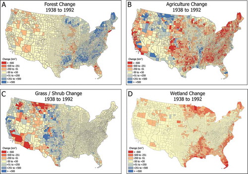
The only other classes that experienced net losses from 1938 to 1992 were the two wetland classes. Both herbaceous and woody wetland classes declined from 1938 to 1992, with the greatest rates of decline occurring early in the simulation period. Wetland loss from 1938 to 1992 was concentrated in three major areas: 1) the upper Midwest (in Minnesota, Wisconsin, Michigan, Ohio, and Illinois), 2) Florida and the southeastern Atlantic coast, and 3) the Mississippi Alluvial Plain (lower Mississippi River) and the adjacent Texas and Louisiana Gulf Coast. Less substantial and more local concentrations of wetland loss include the Central Valley of California and coastal areas along the Atlantic shoreline.

The highest net gains over time were collective gains in the three forest classes. The vast majority of forest gains occurred in the eastern US as a result of cropland abandonment (shown as concentrations of change in the southeastern and northeastern US in Figure 3) Grassland also experienced strong gains, primarily resulting from abandonment or conversion of agricultural land uses in the Great Plains. Urban area expanded dramatically, covering nearly 100,000 km² (140%) more in 1992 than in 1938. The substantial increase in water area was primarily due to modeled reservoir construction between 1938 and 1992, contributing to a 46,200 km² (25%) increase in area.

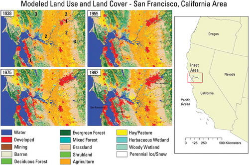
Figure 4 depicts the full-resolution, modeled 1938–1992 change for an area near San Francisco, California. Urban expansion is evident in many areas, including in the San Francisco Bay area, but also in Sacramento and other areas in the Central Valley of California (the heavily agricultural area in the eastern half of the image). Agricultural land extent (both cropland and hay/pasture) was substantially greater in 1938 than at present (with modeled change mimicking records from the Agricultural Census data), particularly around the margins of the Central Valley. A number of reservoirs were constructed during the time period, with the model ‘removing’ them at appropriate dates as FORE-SCE iterated backwards in time.

Figure 4. Modeled LULC from 1938 to 1992 for the San Francisco, California area. Major LULC changes noted include 1) areas of urbanization, 2) areas of agricultural loss, and 3) reservoir construction.

3.1. Assessment of modeled LULC maps

3.1.1. Overall disagreement – comparison with trends data

Figure 5 depicts pixel-level agreement and disagreement measures between modeled data and Trends sample block data for the 84 Level III ecoregions in the conterminous US, for the earliest and latest Trends dates (1973 and 1992, respectively). Agreement and disagreement measures vary little between 1992, the start of the simulation period, and 1973, the earliest Trends date. Median agreement at the pixel level for all ecoregions is 75.6% in 1992, prior to the initiation of FORE-SCE model runs (essentially representing pixel-level differences between the modified 1992 NLCD and the 1992 Trends data). After 19 annual model iterations (back to 1973), median pixel-level agreement declined only slightly to 75.2%. Quantity disagreement represents approximately 20% of the total disagreement at both the start of the simulation period, and in the modeled 1973 data. FORE-SCE is designed to match input LULC proportions to a very high degree, and thus quantity disagreement would not be expected to decline from 1992 back to 1973. Allocation disagreement, representing approximately 80% of all disagreement at the start of the simulation period, is dominated by the exchange disagreement component. Model runs were parameterized at the ecoregion scale, and thus the change in allocation disagreement from 1992 back to 1973 represents how well the model distributed LULC change spatially across each ecoregion, in comparison to reference Trends sample blocks. Median, minimum, and maximum values for each of the individual disagreement measures vary little between 1992 and 1973 among the 84 ecoregions. Clearly the initial pixel-level differences between the 1992 NLCD and 1992 Trends data represent the majority of disagreement, with the modeling from 1992 back to 1973 only introducing a small amount of additional disagreement.

Figure 5. Agreement and disagreement measures between modeled data and USGS Land Cover Trends data for the 84 Level III ecoregions in the conterminous United States. Disagreement is broken down into Quantity Disagreement, and the two elements of Allocation Disagreement (Exchange and Shift).

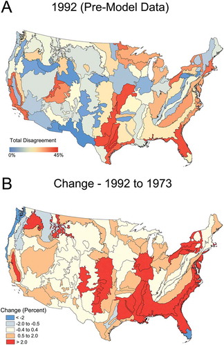
Figure 6 portrays the total disagreement (modeled data versus Trends) for each of the 84 Level III ecoregions for 1992, as well as the change in those measures in the 1973 modeled date. The total disagreement at the pixel level varies from 8 to 44% among ecoregions in 1992, before modeling began (Figure 6, Panel A). The modeling from 1992 back to 1973 results in modest increases in the total disagreement in approximately half of the 84 ecoregions (maximum increase of 4.4%), although disagreement actually declines for several ecoregions (Figure 6, Panel B). Given FORE-SCE’s ability to closely match prescribed quantitative proportions of LULC change, most of the introduced modeled disagreement is pixel-level allocation disagreement with reference Trends data. This tends to occur most often in ecoregions with a high amount of modeled change (compare to Figure 4). There is little evidence of increased disagreement between areas modeled explicitly as level III ecoregions and those modeled as part of broader level II ecoregions (see the discussion below).

Figure 6. Total disagreement measures by ecoregion for 1992, and change from 1992 to 1973. Panel A depicts the total disagreement for 1992, representing initial disagreement between the modified 1992 NLCD and the Trends sample blocks. Panel B depicts the percent change in the total disagreement between the modeled and Trends 1973 data.

3.1.2. Sector: agriculture

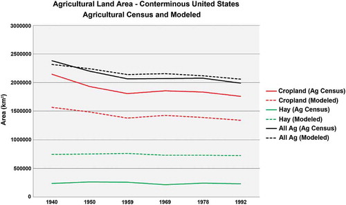
Figure 7 depicts area of cropland, hay/pasture, and total agriculture (cropland and hay/pasture combined) as modeled, and for the Agricultural Census data. The total agriculture area is similar between the two at the start of the simulation period, with the modified 1992 NLCD and 1992 Agricultural Census data matching closely. The split between what is classed as cropland or hay/pasture is where substantial differences exist between the two starting 1992 datasets. Despite the close match in the total agriculture, NLCD has much more hay/pasture and much less cropland than measured by the Agricultural Census. By using proportional rates of change from the Agricultural Census but applying them to our starting land cover proportions from the 1992 NLCD, we are in effect capturing the primary ‘story’ of agricultural change, despite the difficulties in harmonizing our historical input data sources.

Figure 7. Total area of cropland, hay/pasture, and total agriculture (cropland and hay/pasture) throughout the 1938–1992 simulation period, compared to Agricultural Census data.

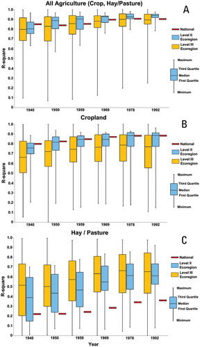
Figure 8 represents r² values between modeled and Agricultural Census data at the county level for the total agriculture, and the cropland and hay/pasture components, at different spatial scales. A national r² value was calculated, as were r² values for all ecoregions at the Level II scale (n = 15) and at the Level III scale (n = 84). The goal was to determine how well FORE-SCE distributed agricultural change spatially by providing an overall quantitative measure of a county-level match between modeled and Agricultural Census data. The total agriculture (Panel 8-A) has r² of 0.90 in 1992, representing the agreement of the starting 1992 NLCD and the 1992 Agricultural Census at a county level. The r² shows a modest decline to 0.85 by 1938, a significant (p < 0.05) yet modest decrease in agreement between the modeled LULC map and Agricultural Census data at the county level. For the individual cropland component (Panel 8-B), r² is slightly lower than that for the total agriculture (0.88 versus 0.90 for 1992) and shows a modest yet significant (p < 0.05) decline to 0.80 for 1938. At a national scale, the agreement is much poorer for hay/pasture from the start of the simulation period (Panel 8-C). The 1992 r² for hay/pasture is 0.37, declining steadily to 0.22 by 1938. Regional r² values in Figure 8 vary substantially between ecoregions. For the total agriculture, variability between ecoregions is modest for the 15 Level II ecoregions, but rises substantially for the 84 Level III ecoregions, with some level III ecoregions showing extremely high r² values, and some showing very low values. Variability between both ecoregion scales rises when agriculture is broken down into the cropland and hay/pasture classes, again with some ecoregions showing a close match, and others a poor match at a county level. On average, r² values show modest (yet statistically significant) declines as the model iterates backwards in time at all scales. Overall however, the level of decline is smaller than is the overall disagreement between the NLCD and Agricultural Census data at the start of the simulation period in 1992.

Figure 8. Boxplots of county-level r² values between modeled LULC and the Agricultural Census data for cropland, hay/pasture, and total agriculture for all counties (national, Panel A), and for Level II (n=15, Panel B) and Level III (n=84, Panel C) ecoregions. Counties were assigned to ecoregions containing the largest areal proportion of that county.

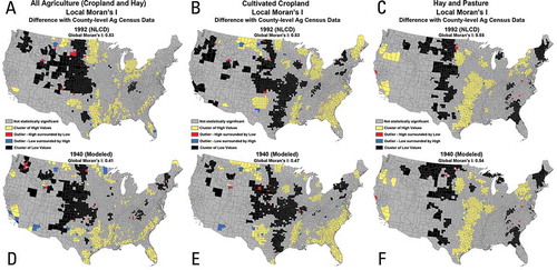
Figure 9 depicts spatial patterns of disagreement across the conterminous US, when comparing modeled agricultural classes versus the Agricultural Census data by county. Global Moran’s I values for the start of the simulation period indicate significant (p < 0.01) spatial autocorrelation between modeled LULC and Agricultural Census data. In short, significant clusters of disagreement between the 1992 NLCD and the Agricultural Census data exist, prior to any FORE-SCE model runs (Figure 9A, 9B, 9C). In some areas, the total agriculture matches well, with the individual components of cropland and hay/pasture not matching well but appearing to ‘balance out’. For example, cropland in 1992 is underrepresented in the 1992 NLCD compared to the 1992 Agricultural Census in a large swath of the south-central US, while hay/pasture is overpredicted in the same general area. This pattern reinforces the values shown in Figure 7, indicating that the starting NLCD tends to show higher levels of cropland and lower levels of hay/pasture compared to Agricultural Census data. Figure 9 also shows a high level of similarity between local Moran’s I maps for both 1992 (top row) and 1940 (bottom row). For the total agriculture and for the individual cropland and hay/pasture components, the similarity in patterns between 1992 and 1940 maps again suggests that the spatial allocation component of FORE-SCE is not introducing substantial new patterns of disagreement that were not already present in the starting 1992 data.

Figure 9. Local Moran’s I of the difference between modeled and Agricultural Census values for the total agriculture, cropland, and hay/pasture, for 1992 and 1938. ‘Cluster of High Values’ represents areas with a statistically significant cluster of overpredicted values (i.e., modeled values higher than Agricultural Census). ‘Cluster of Low Values’ represents areas with a statistically significant cluster of underpredicted values. ‘Outlier – High surrounded by Low’ represents a county with a significantly higher overprediction compared to surrounding counties. ‘Outlier – Low surrounded by High’ represents a count with a significantly lower underprediction compared to surrounding counties.

3.1.3. Sector: urban

Figure 10 provides a comparison of modeled urban area versus Trends estimates (1973–1992), and housing density data (1940–2000 shown). Trends estimates at a national scale are considerably higher than modeled or housing density data. Trends used an intensive manual interpretation procedure to map LULC for each sample block and captured low density developed lands that are difficult to map from remote sensing imagery. The starting 1992 NLCD data used in this assessment thus had a considerably lower proportion of urban lands compared to Trends. As expected, the rate of decline in modeled urban area closely matched the estimated rate of change from Trends, and also closely matched the rate of decline from the historical housing density data going back to 1938.

Figure 10. Urban/developed area for the conterminous US as modeled, and for Trends and Housing Density data. Housing density represents areas with > 100 housing units per km2.

3.1.4. Sector: grassland/shrubland

Grassland and shrubland were ‘passively’ modeled, with changes in these two classes resulting from modeled changes in the better quantified agricultural, urban, wetland, and reservoir classes. For the 1973–1992 period, the Trends data (Sleeter et al., 2013) show a minor decline in grassland/shrubland from 1973 to 1986 followed by an increase in area (influenced by the establishment of the Conservation Reserve Program (CRP) after 1985), a pattern similar to these model results (Figure 11). Data from the US Department of Agriculture’s Economic Research Service (USDA-ERS) (Luhowski et al., 2006) provide a combined grassland, pasture, and range class. This class from USDA-ERS and our modeled grassland and shrubland data both show a general decline from 1945 to present, although the rate of decline is substantially greater in the Lubowski, Vesterby, Bucholtz, Baez, and Roberts, (2006) data. The USDA-ERS data do not depict the CRP-influenced rise in grassland/shrubland that is shown in the Trends data and these modeled results, yet most studies do indicate a decline in cropland and resultant increase in grassland after implementation of CRP (Coppedge, Engle, Fuhlendorf, Masters, & Gregory, 2001; Egbert et al., 2002; Johnson & Schwartz, 1993).

Figure 11. ‘Passively’ modeled trends in grassland/shrubland and forest classes, and a comparison with Trends (Sleeter et al. 2013), Smith et al. (2004), and Lubowski et al. (2006) data. The modeled and Trends results show combined grassland and shrubland data, while Luboski et al. (2006) depicts a grassland, pasture, and range class. Deciduous, evergreen, and mixed forest classes were combined from these results to compare to the single ‘forest’ class from Trends and Smith et al. (2004).

3.1.5. Sector: forest

Modeled results for the three combined ‘forest’ classes show strong increases in forest area from 1938 to about 1962, followed by a relatively stable trend through the rest of the study period. The Trends data (Sleeter et al., 2013) from 1973 to 1992 show a steady decline in forest area, while the modeled results from 1973 to 1992 show a decline followed by a slow increase (Figure 11). Smith et al. (2004) depicted a different trend in forest area compared to the modeled results, with stability from 1938 through about 1970, followed by a slow decline. In general, the forest sector shows greater differences compared with an exogenous data source (Smith et al., 2004) than do the other classes. A discussion of the differences in forest trends is found below.

4. Discussion

Using the best available historical data sources on LULC change for the conterminous US, we produced a unique set of annual, moderate spatial-resolution and thematic resolution LULC maps for the US from 1938 to 1992. The modeling approach necessarily focused on the active modeling of the anthropogenic LULC classes of agriculture, urban, and reservoirs, classes with the highest quality, spatially explicit data available for the modeled time period. In combination with historical information on wetland drainage, the actively modeled LULC classes in this assessment accounted for the vast majority of land use changes that occurred between 1938 and 1992. Grassland, shrubland, and the multiple forest classes were passively modeled, with changes resulting from the actively modeled anthropogenic classes. An exact pixel-level recreation of historical LULC may not be practical or possible, but this approach does provide a practical means for producing spatially explicit, moderate thematic and spatial resolution LULC projections that capture overall historical stories of LULC change at a regional level.

While we were able to quantitatively (and spatially) assess modeled changes in the actively modeled agricultural and urban classes, the question does arise whether the passively modeled ‘natural’ classes of grassland, shrubland, and forest were well represented. While data availability largely drove the decision to passively model most natural land covers, the decision was also based on the assumption that the availability of natural LULC classes is largely based on the ebb and flow of anthropogenic activity in a region. For example, in the Great Plains, the amount of land actively cultivated has changed over the years in response to favorable or unfavorable economic conditions for agricultural commodities (Johnston, 2014; Joyce et al., 1991; Rashford et al., 2010). In favorable periods, cultivated agriculture expands at the expense of grassland throughout much of the Great Plains, while the opposite occurs in unfavorable periods. Similarly, agriculture in the southeastern US (and eastern US as a whole) has declined during the study period with substantial ‘natural’ forest LULC increases as forests regenerated on abandoned agricultural land (Brown et al., 2005; Ramankutty, Heller, & Rhemtulla, 2010). Unlike the Great Plains, cropland change in the eastern US has been more unidirectional, generally occurring as a one-time loss of cropland as it is abandoned and regenerates to forest.

Grassland/shrubland trends were similar to the few comparable data sources (Figure 11), although the magnitude of change in USDA-ERS data was certainly higher. There are no clear explanations for differences between the USDA-ERS, Trends, and modeled data, but definitional differences likely are a major contributing factor. Combining the grassland and shrubland classes from the modeled data allowed for fairly straightforward comparison with the Trends data. However, the USDA-ERS estimates were for a ‘grassland, pasture, and range’ class that focused heavily on anthropogenic land use, while Trends data and the modeled data (starting from 1992 NLCD) used maps focused on land covers of grassland and shrubland. Definitional differences not only occur between datasets, but also within a single dataset. USDA-ERS notes definitional changes in their land use data that often preclude revision for prior dates, leading to abrupt changes between dates that do not represent real land use change (Lubowski et al. 2006). Definitional differences, both within and between datasets, confound trend assessments and dataset comparison for other classes as well, as discussed below.

Of all LULC sectors, the forest sector results differed the most from a historical data sources (i.e., comparison with Smith et al., 2004 in Figure 11). As with grassland and shrubland, definitional differences may contribute to differences in forest trends compared to Smith et al. (2004). For example, it is unclear how ‘forested wetland’ is categorized in Smith et al. (2004). If we include forested wetland as ‘forest’, the ~60,000 km² of forested wetland loss in Table 1 would result in approximately a one-third reduction in the overall forest gain we model from 1938 to 1992. This potential definitional adjustment brings these results closer to Smith et al. (2004), but the remaining forest gain still disagrees with the Smith et al. (2004) results. Note that historical sources other than Smith et al. (2004) often portray a common narrative for forest in the US of massive forest cutting through the nineteenth and early twentieth century, followed by substantial forest expansion through the twentieth century as abandoned agricultural land regenerated to forest (Clawson, 1979; Drummond & Loveland, 2008; Williams, 1989). Hart (1968) summarized historical agricultural and forest change in the eastern US from 1910 to 1959, and depicted spatial patterns of historical farmland loss and implied forest gain (Figures 3 and 4 of that study) similar to spatial results shown here (Figure 3). These results clearly agree with the storyline of widespread cropland loss and forest gain from multiple sources, but Ramankutty et al. (2010) argue that there are flaws with the storyline. Ramankutty et al. (2010) noted a definitional shift in the Agricultural Census in the early 1940s that potentially explains the very large jump in the ‘total cropland’ estimates prior to that date. Ramankutty et al. (2010) also pointed to the Smith et al. (2004) data which show only modest forest change during the twentieth century as evidence to challenge the traditional story of massive cropland loss and forest gain in the US.

If we assume little agricultural change in the earliest 1938–1945 period, as per Ramankutty et al. (2010), our overall cropland change from 1938 to 1992 agrees strongly with their results. However, even if Ramankutty et al. (2010) are correct in assuming the cropland loss in the earliest time frame is an artificial relict of a definition change in the Agricultural Census data, it does not explain our modeled forest increases after the mid-1940s, increases not present in the Smith et al. (2004) forest area estimates. From Table 1, ~60% of all forest gains (~120,000 km²) occur from 1948 to 1992, after any influence (i.e., cropland abandonment resulting in forest gains) of definitional changes in the Agricultural Census data. The major reason for this gain is the location of reported cropland loss in these data. In the study period’s first 10 years, substantial cropland loss occurs in both the Great Plains and the eastern US; thus, approximately half of all conterminous US cropland loss ends up converting to grassland or shrubland (most conversions in the Great Plains), and approximately half converts to forest (most conversions in the eastern US). However, after 1948, the vast majority of all cropland loss occurs in the (largely forested) eastern United States, while cropland is generally stable or locally declining west of the Mississippi River (Brown et al., 2005; Waisanen & Bliss, 2002). Some of the cropland loss in the East occurs when cropland is converted to urban land use, but there is not nearly enough urbanization to account for all cropland loss estimated by the Agricultural Census. There is very little grassland or shrubland in the eastern US in the 1992 NLCD; it is primarily forest, wetland, agricultural, and urban classes. Looking at it in reverse, as we model backwards in time and need to add large amounts of cropland in the eastern US, forested land covers simply must make up a majority of those conversions, explaining the large increase in forested land looking forward from 1938 to 1992. The much smaller forest losses west of the Mississippi River (primarily due to urbanization) are not nearly enough to change the overall storyline of forest gain from 1938 to 1992 in the conterminous US.

The question arises: who is ‘right’? Past studies have noted disparities in LULC datasets resulting from different thematic classification schemes, scales, and mapping methodologies (Herold et al., 2008; Verburg et al., 2011), and the challenges these differences pose. Laingen (2015) recently noted vast differences in LULC classification results between data sources based on surveys, satellite-based sensors, or aerial photography. For this study, the Smith et al. (2004) forest data (showing no substantial forest change over the study period), the Agricultural Census data (used to parameterize these model runs), and our starting 1992 NLCD are not easily reconcilable. Given the large cropland loss in the Agricultural Census data throughout the 1938–1992 time period and given measured areas of urbanization, there simply is no large LULC pool for cropland to ‘convert into’ as you go forward in time in the eastern US, other than forested land uses. Overall, definitional differences between source datasets (and with our modeled classification scheme), different methodologies used for data collection (e.g., field-based versus remote sensing estimates), and a focus on land use vs. land cover confound an ability to reconcile historic LULC datasets and provide one coherent land use history for the conterminous US. By choosing to rely heavily on the Agricultural Census data (one of the few spatially explicit historical LULC data sources for the conterminous US.) to serve as a primary data source for parameterizing our model, we committed to any assumptions and biases associated with that dataset. Given the logical discrepancies between datasets, the use of Agricultural Census data thus commits us to disagree with stated national trends from other datasets.

As noted in the methodology section, the base ecoregion framework was altered midway through the project, with the central US parameterized and modeled at the Level III ecoregion scale, and the rest of the US modeled at the coarser Level II ecoregion scale. The move toward a coarser spatial framework raised concerns about a potentially poorer spatial match of modeled data with reference data sources. Model runs based on Level II ecoregion scales relied on demand aggregated across broader geographic areas than model runs based on Level III ecoregions, potentially straining FORE-SCE’s ability to properly spatially allocate LULC change across the broader area. When comparing modeled 1973 data to the reference 1973 Trends sample block data at a pixel level, however, final model results showed little variability in disagreement measures whether a region was modeled at the Level II or Level III ecoregion scale. Changes in the total disagreement between 1992 and 1973 were not significantly different for explicitly modeled Level III ecoregions than for Level III ecoregion areas modeled within a coarser Level II ecoregion framework (p = 0.61). Given the lack of spatially explicit reference data prior to 1973, it is possible that for longer modeling time periods, spatial disagreement measures could increase more substantially for ecoregions modeled with the coarser spatial framework. However, comparisons to available reference data are encouraging in terms of confidence in consistency of national-level results, regardless of what scale of ecoregion was used for parameterization.

One of the greatest challenges for this assessment was trying to harmonize the modified 1992 NLCD, Trends, and Agricultural Census data, as each provided different estimates of proportional US land cover from the start of the simulation period in 1992. Those differences obviously affected not only our modeling methodology, but the interpretation of the tools used to assess modeling results. Figures 5 and 6 indicate substantial disagreement between the starting 1992 NLCD and Trends data at a pixel level. It is likely that resampling issues and a comparison of the native 60-m Trends data to the native 250-m modeled data resulted in a small amount of pixel-level disagreement, but not the overall broad discrepancies between the datasets in 1992. A simple graph of starting LULC proportions also revealed the variation in agricultural classes between the starting 1992 NLCD and the Agricultural Census data (Figure 7). It is thus impossible to interpret the assessment measures provided in this article without the context of initial disagreement present between the different data sources. Absolute disagreement measures, or assessment of the spatial patterns of model results, cannot be interpreted directly as characterizing modeling success or failure. Assessment measures provided here do indicate modest degradation in agreement with other historical data sources as the model iterates backwards in time. However, the amount of degradation in all measures is generally much smaller than any disagreement that is present in 1992, before the modeling even began.

5. Conclusion

While existing data such as Trends, Agricultural Census, or drained lands data provide information on historical LULC change for the conterminous US, they are either 1) sample based (e.g., Trends spatially explicit sample blocks, but with coverage of less than 3% of the conterminous US area), 2) cover only a limited set of LULC classes (e.g., Agricultural Census data that provide extensive information on agricultural land use but do not capture other land use categories), and/or 3) do not provide spatially explicit information (Agricultural Census, drained lands that provide only aggregate level estimates at county or coarser-level resolution). These data represent the first spatially explicit, moderate resolution, high thematic detail LULC data for the entire conterminous US for dates prior to the Landsat satellite era. Using a practical modeling methodology parameterized at the broad ecoregion scale, we have produced historical LULC maps that agree spatially with historical trends in LULC. Tthe results closely mimic rates of change measured by historical data sources such as the Trends and Agricultural Census data. By producing wall-to-wall annual LULC data at higher spatial and thematic resolution than other LULC currently available for the conterminous US, we have improved the capabilities of researchers to assess historical impacts of LULC changes on a host of ecological processes. In combination with the 1992–2100 LULC database previously produced (Sohl et al., 2014), researchers can use LULC data from the historical period to reveal connections between LULC change and phenomenon related to hydrology, biodiversity, climate, and biogeochemical cycling, and use that information to better understand the potential future consequences of LULC change on those processes.

A secondary finding from this work is demonstrating the difficulties in validating historical maps, or even just reconciling all historical data sources and deriving one consistent storyline of change. Methodological and definitional differences hinder even basic comparisons between historical data sources. Given the logical inconsistencies apparent when trying to reconcile all historical data sources, care is necessary when trying to draw conclusions based on any one historical dataset, a finding also noted by others (Ramankutty et al., 2010).

The 250-m, annual LULC maps from 1938 to 1992 are freely available for download and use, as are the 1992–2100 scenario-based data. These data and other information on FORE-SCE modeling activities at USGS EROS may be accessed at http://www.landcover-modeling.cr.usgs.gov.

Disclosure statement

No potential conflict of interest was reported by the authors.

References

- Anselin, L. (1995). Local indicators of spatial association – LISQA. Geographical Analysis, 27, 93–115. doi:10.1111/j.1538-4632.1995.tb00338.x
- Askins, R. A., Chávez-Ramírez, F., Dale, B. C., Haas, C. A., Herkert, J. R., Knopf, F. L., & Vickery, P. D. (2007). Ornithological Monographs No. 64, Conservation of Grassland Birds in North America: Understanding Ecological Processes in Different Regions: Report of the AOU Committee on Conservation (2007), pp. iii-viii, 1-46.
- Birdsey, R., Pregitzer, K., & Lucier, A. (2006). Forest carbon management in the United States: 1600-2100. Journal of Environment Quality, 35, 1461–1469. doi:10.2134/jeq2005.0162
- Brown, D. G., Johnson, K. M., Loveland, T. R., & Theobald, D. M. (2005). Rural land-use trends in the conterminous United States, 1950-2000. Ecological Applications, 15(6), 1851–1863. doi:10.1890/03-5220
- Chase, T. N., Pielke, R. A., Sr., Kittel, T. G. F., Nemani, R. R., & Running, S. W. (2000). Simulated impacts of historical land cover changes on global climate in northern winter. Climate Dynamics, 16(2–3), 93–105. doi:10.1007/s003820050007
- Clawson, M. (1979). Forests in the long sweep of American history. Science, 204, 1168–1174. doi:10.1126/science.204.4398.1168
- Coppedge, B. R., Engle, D. M., Fuhlendorf, S. D., Masters, R. E., & Gregory, M. S. (2001). Landscape cover type and pattern dynamics in fragmented southern great plains grasslands. USA. Landscape Ecology, 16, 677–690. doi:10.1023/A:1014495526696
- Dahl, T. E., & Allord, G. J. (1996). Technical aspects of wetlands: History of wetlands in the conterminous United States. In J. D. Fretwell, J. S. Williams, & P. J. Redman (Eds.), National water summary on wetland resources. U.S. Geological Survey Water-Supply Paper 2425 (pp. 19–26). Washington, DC: U.S. Government Printing Office.
- Drummond, M. A., & Loveland, T. R. (2008). Land-use pressure and a transition to forest-cover loss in the Eastern United States. BioScience, 60(4), 286–298. doi:10.1525/bio.2010.60.4.7
- Egbert, S. L., Park, S., Price, K. P., Lee, R.-Y., Wu, J., & Nellis, M. D. (2002). Using conservation reserve program maps derived from satellite imagery to characterize landscape structure. Computers and Electronics in Agriculture, 37(1–3), 141–156. doi:10.1016/S0168-1699(02)00114-X
- Falcone, J. A. (2015). U.S. conterminous wall-to-wall anthropogenic land use trends (NWALT), 1974–2012: U.S. Geological Survey Data Series 948, pp. 33, 10.3133/ds948
- Frans, C., Istanbulluoglu, E., Mishra, V., Munoz-Arriola, F., & Lettenmaier, D. P. (2013). Are climatic or land cover changes the dominant cause of runoff trends in the Upper Mississippi River Basin? Geophysical Research Letters, 40(6), 1104–1110. doi:10.1002/grl.v40.6
- Fry, J. A., Xian, G., Jim, S., Dewitz, J. A., Homer, C. G., Yang, L., … Wickham, J. D. (2011). Completion of the 2006 national land cover database for the conterminous United States. Photogrammetric Engineering and Remote Sensing, 77(9), 858–864.
- Fuchs, R., Herold, M., Verburg, P. H., Clevers, J. G. P. W., & Eberle, J. (2014). Gross changes in reconstructions of historic land cover/use for Europe between 1900 and 2010. Global Change Biology. doi:10.1111/gcb.12714
- H. John Heinz III Center for Science, Economics, & the Environment. (2002). The state of the nation’s ecosystems: Measuring the lands, waters, and living resources of the United States. Cambridge: Cambridge University Press.
- Hart, J. F. (1968). Loss and abandonment of cleared farm land in the eastern United States. Annalys of the Association of American Geographers, 58(3), 417–440. doi:10.1111/j.1467-8306.1968.tb01645.x
- Herold, M., Mayaux, P., Woodcock, C. E., Baccini, A., & Schmullius, C. (2008). Some challenges in global land cover mapping: An assessment of agreement and accuracy in existing 1 km datasets. Remote Sensing of Environment, 112, 2538–2556. doi:10.1016/j.rse.2007.11.013
- Hurtt, G. C., Chini, L. P., Frolking, S., Betts, A., Feddema, J., Fischer, G. … Wang, Y. P. (2011). Harmonization of land-use scenarios for the period 1500-2100: 600 years of global gridded annual land-use transitions, wood harvest, and resulting secondary lands. Climatic Change, 109(1–2), 117–161. doi:10.1007/s10584-011-0153-2
- Johnson, D. H., & Schwartz, M. D. (1993). The conservation reserve program: Habitat for grassland birds. Great Plains Research, 3, 273–295.
- Johnston, C. A. (2014). Agricultural expansion: Land use shell game in the U.S. northern plains. Landscape Ecology, 29, 81–95. doi:10.1007/s10980-013-9947-0
- Joyce, L. A., Mitchell, J. E., & Skold, M. D. (Eds.) (1991). The conservation reserve – yesterday, today, and tomorrow. USDA Forest Service General Technical Report RM-203. Fot Collins, CO: USDA Rocky Mountain Forest and Range Experiment Station.
- Laingen, C. (2015). Measuring cropland change: A cautionary tale. Papers in Applied Geography, 1(1), 65–72. doi:10.1080/23754931.2015.1009305
- Loveland, T. R., Sohl, T. L., Stehman, S. V., Gallant, A. L., Sayler, K. L., & Napton, D. E. (2002). A strategy for estimating the rates of recent United States land-cover changes. Photogrammetric Engineering and Remote Sensing, 68, 1091–1099.
- Lubowski, R. N., Vesterby, M., Bucholtz, S., Baez, A., & Roberts, M. J. (2006). Major uses of land in the United States, 2002. Washington, DC: Economic Information Bull. 14. USDA, Economic Research Service.
- Moran, P. A. P. (1950). Notes on continuous stochastic phenomena. Biometrika, 37(1–2), 17–23. doi:10.1093/biomet/37.1-2.17
- Pielke, R. A., Sr., Pitman, A., Niyogi, D., Mahmood, R., McAlpine, C., Hossain, F. … De Noblet, N. (2011). Land use/land cover changes and climate: Modeling analysis and observational evidence. Climate Change, 2(6), 828–850.
- Pontius, R. G., Jr., & Millones, M. (2011). Death to Kappa: Birth of quantity disagreement and allocation disagreement for accuracy assessment. International Journal of Remote Sensing, 32, 4407–4429. doi:10.1080/01431161.2011.552923
- Pontius, R. G., Jr., & Santacruz, A. (2014). Quantity, exchange, and shift components of difference in a square contingency table. International Journal of Remote Sensing, 35(21), 7543–7554. doi:10.1080/2150704X.2014.969814
- Protected Areas Database of the United States (PAD–US) Partnership. (2009). A map for the future—Creating the next generation of protected area inventories in the United States: Protected Areas Database of the United States Partnership. 20 p., Retrieved June 18, 2011, from http://www.protectedlands.net/images/PADUS_FinalJuly2009LowRes.pdf
- Radeloff, V. C., Hagen, A. E., Voss, P. R., Field, D. R., & Mladenoff, D. J. (2000). Exploring the spatial relationship between census and land cover data. Society and Natural Resources, 13(6), 599–609. doi:10.1080/08941920050114646
- Ramankutty, N., & Foley, J. A. (1999). Estimating historical changes in global land cover: Croplands from 1700 to 1992. Global Biogeochemical Cycles, 13(4), 997–1027. doi:10.1029/1999GB900046
- Ramankutty, N., Heller, E., & Rhemtulla, J. (2010). Prevailing myths about agricultural abandonment and forest regrowth in the United States. Annals of the Association of American Geographers, 100(3), 502–512. doi:10.1080/00045601003788876
- Rashford, B. S., Walker, J. A., & Bastian, C. T. (2010). Economics of grassland conversion to cropland in the prairie pothole region. Conservation Biology, 25(2), 276–284.
- Ray, D. K., & Pijanowski, B. C. (2010). A backcast land use change model to generate past land use maps: application and validation at the Muskegon river watershed of Michigan, USA. Journal of Land Use Science, 5(1), 1–29. doi:10.1080/17474230903150799
- Rollins, M. G. (2009). LANDFIRE: A nationally consistent vegetation, wildland fire, and fuel assessment. International Journal of Wildland Fire, 18(3), 235–249. doi:10.1071/WF08088
- Samson, F. B., Knopf, F. L., & Ostlie, W. R. (2004). Great plains ecosystems: Past, present, and future. Wildlife Society Bulletin, 32(1), 6–15. doi:10.2193/0091-7648(2004)32[6:GPEPPA]2.0.CO;2
- Sleeter, B. M., Sohl, T. L., Bouchard, M. A., Reker, R. R., Soulard, C. E., Acevedo, W. … Zhu, Z. (2012). Scenarios of land use and land cover change in the conterminous United States: Utilizing the special report on emission scenarios at ecoregional scales. Global Environmental Change, 22, 896–914. doi:10.1016/j.gloenvcha.2012.03.008
- Sleeter, B. M., Sohl, T. L., Loveland, T. R., Auch, R. F., Acevedo, W., Drummond, M. A. … Stehman, S. V. (2013). Land-cover change in the conterminous United States from 1973 to 2000. Global Environmental Change, 23(4), 733–748. doi:10.1016/j.gloenvcha.2013.03.006
- Smith, B. W., Miles, P. D., Vissage, J. S., & Pugh, S. A. (2004). Forest Resources of the United States, 2002: A Technical Document Supporting the USDA Forest Service 2005 Update of the RPA Assessment. General Technical Report NC-241. St. Paul, MN: U.S. Department of Agriculture, Forest Service, North Central Research Station. http://ncrs.fs.fed.us/pubs/gtr/gtr_nc241.pdf.
- Sohl, T. L., Sayler, K. L., Bouchard, M. A., Reker, R. R., Friesz, A. M., Bennett, S. L. … Knuppe, M. (2014). Spatially explicit modeling of 1992 to 2100 land cover and forest stand age for the conterminous United States. Ecological Applications, 24(5), 1015–1036. doi:10.1890/13-1245.1
- Sohl, T. L., Sayler, K. L., Drummond, M. A., & Loveland, T. R. (2007). The FORE-SCE model: A practical approach for projecting land cover change using scenario-based modeling. Journal of Land Use Science, 2(2), 103–126. doi:10.1080/17474230701218202
- Sohl, T. L., Sleeter, B. M., Zhu, Z., Sayler, K. L., Bennett, S., Bouchard, M. … Acevedo, W. (2012). A land-use and land-cover modeling strategy to support a national assessment of carbon stocks and fluxes. Applied Geography, 34, 111–124. doi:10.1016/j.apgeog.2011.10.019
- Steyaert, L. T., & Knox, R. G. (2008). Reconstructed historical land cover and biophysical parameters for studies of land-atmosphere interactions within the eastern United States. Journal of Geophysical Research, 113, D02101. doi:10.1029/2006JD008277
- Tian, H., Chen, G., Zhang, C., Liu, M., Sun, G., Chappelka, A. … Pan, S. (2012). Century-scale responses of ecosystem carbon storage and flux to multiple environmental changes in the Southern United States. Ecosystems, 15(4), 674–694. doi:10.1007/s10021-012-9539-x
- Trueman, M., Hobbs, R. J., & Van Niel, K. (2013). Interdisciplinary historical vegetation mapping for ecological restoration in Galapagos. Landscape Ecology, 28, 519–532. doi:10.1007/s10980-013-9854-4
- U.S. Army Corps of Engineers. Accessed. (2012). National Inventory of Dams. http://geo.usace.army.mil/pgis/f?p=397:1:0
- U.S. Bureau of the Census. (1932). Fifteenth census of the United States: 1930. Drainage of agricultural lands. Washington, DC: U.S. Government Printing Office.
- U.S. Bureau of the Census. (1935). U.S. Census of Agriculture. 1935, vol. I, Reports for States with Statistics for Counties and a Summary for the United States: Farms, Farm Acreage and Value, and Selected Livestock and Crops, Parts 1, 2, 3, U.S. Government Printing Off., Washington, DC, 1936.
- U.S. Bureau of the Census. (1942). Sixteenth census of the United States: 1940. Drainage of agricultural lands. Washington, DC: U.S. Government Printing Office.
- U.S. Bureau of the Census. (1952). U.S. census of agriculture: 1950. Drainage of agricultural lands. Washington, DC: U.S. Government Printing Office.
- U.S. Bureau of the Census. (1961). U.S. census of Agriculture: 1959. Drainage of agricultural lands. Washington, DC: U.S. Government Printing Office.
- U.S. Census Bureau. (1992). U.S. census of agriculture, 1992 [CD-ROM], geographic area series 1A, 1B, and 1C, cross-tab data file and county level data. 1995. Washington, DC: U.S. Government Printing Off.
- U.S. Census Bureau. (2012). TIGER/line shapefile, military installation national Shapefile. Washington, DC: U.S. Census Bureau, Geography Division, Geographic Products Branch.
- U.S. Environmental Protection Agency (EPA). (1999). Level III Ecoregions of the Continental United States. In T. R. Karl, J. M. Melillo, & T. C. Peterson Eds., National health and environmental effects research laboratory, scale 1:7,500,000. Corvallis, Oregon: U.S. Environmental Protection Agency.
- Verburg, P. H., Neumann, K., & Nol, L. (2011). Challenges in using land use and land cover data for global change studies. Global Change Biology, 17, 974–989. doi:10.1111/gcb.2010.17.issue-2
- Vogelmann, J. E., Howard, S. M., Yang, L., Larson, C. R., Wylie, B. K., & Van Driel, N. (2001). Completion of the 1990s national land cover data set for the conterminous United States from landsat thematic mapper data and ancillary data sources. Photogrammetric Engineering and Remote Sensing S, 67, 650–662.
- Waisanen, P. J., & Bliss, N. B. (2002). Changes in population and agricultural land in conterminous United States counties, 1790 to 1997. Global Biogeochemical Cycles, 16, 84–1. doi:10.1029/2001GB001843
- Wilcove, D. S., Rothstein, D., Dubow, J., Phillips, A., & Losos, E. (1998). Quantifying threats to imperiled species in the United States. BioScience, 48(8), 607–615. doi:10.2307/1313420
- Williams, M. (1989). Americans and their forests: A historical geography. New York: Cambridge University Press.
- Yang, Q., Tian, H., Friedrichs, M. A. M., Liu, M., Li, X., & Yang, J. (2015). Hydrological responses to climate and land-use changes along the North American East Coast: A 110-year historical reconstruction. Journal of the American Water Resources Association, 51(1), 47–67. doi:10.1111/jawr.12232
- Zhao, S., Liu, S., Sohl, T., Young, C., & Werner, J. (2013). Land use and carbon dynamics in the southeastern United States from 1992 to 2050. Environmental Research Letters, 8(4), 044022. doi:10.1088/1748-9326/8/4/044022
- Zumkehr, A., & Campbell, J. E. (2013). Historical U.S. cropland areas and the potential for bioenergy production on abandoned croplands. Environmental Science & Technology, 47, 3840–3847. doi:10.1021/es3033132