Parcels versus pixels: modeling agricultural land use across broad geographic regions using parcel-based field boundaries

ABSTRACT

Land use and land cover (LULC) change occurs at a local level within contiguous ownership and management units (parcels), yet LULC models primarily use pixel-based spatial frameworks. The few parcel-based models being used overwhelmingly focus on small geographic areas, limiting the ability to assess LULC change impacts at regional to national scales. We developed a modified version of the Forecasting Scenarios of land use change model to project parcel-based agricultural change across a large region in the United States Great Plains. A scenario representing an agricultural biofuel scenario was modeled from 2012 to 2030, using real parcel boundaries based on contiguous ownership and land management units. The resulting LULC projection provides a vastly improved representation of landscape pattern over existing pixel-based models, while simultaneously providing an unprecedented combination of thematic detail and broad geographic extent. The conceptual approach is practical and scalable, with potential use for national-scale projections.

KEYWORDS:

• Land use
• modeling
• parcel
• agriculture
• regional
• FORE-SCE

1. Introduction

Land use and land cover (LULC) models operate at scales from global to local. Most models have been established to address research questions at a particular scale of analysis (Verburg, Van De Steeg, Veldkamp, & Willemen, 2009), and overall, linking drivers of LULC change across multiple scales has been a challenge for LULC modeling (NRC 2013; Rounsevell et al., 2012; Sohl, Loveland, Sleeter, Sayler, & Barnes, 2010). One difficulty lies with the scale of relevant data sources used for LULC modeling as LULC models often default to the native resolution of readily available data sources. With the extensive use of remote sensing to characterize land cover (and increasingly, land use), the pixel remains the primary means by which models depict LULC and LULC change. The argument has been made that LULC science must attempt to ‘link land use to the pixel’ (Rindfuss, Walsh, Turner, Fox, & Mishra, 2004), a practical consideration given the ease of representing LULC change with the most commonly used spatial framework (raster data). However, a primary tenet of geography is that the scale of analysis must match the actual scale of the phenomenon. The native resolution and basic spatial unit (the pixel) associated with a sensor on a remote sensing platform is arbitrary and unrelated to the scale of actual processes that drive LULC change.

LULC models have been critiqued in that the basic unit of analysis is often a pixel, rather than spatial units on which LULC change actually occurs (Ballestores Jr. and Qiu 2012; Irwin & Geoghegan, 2001; National Research Council, 2013). LULC change transpires at the parcel level, with parcels defined as the primary unit of land ownership and management (Brown, Pijanowski, & Duh, 2000). In agricultural landscapes, ownership and management parcels correspond to individual farm fields. Modeling in agricultural landscapes has been done using parcel-based models, but these have primarily been agent-based models or econometric models operating over small geographic extents. Examples of recent parcel-based modeling applications include Pocewicz et al. (2008), who modeled five basic LULC classes for two counties (~4,800 km²) in Idaho, Ballestores Jr. and Qiu (2012), who modeled six LULC classes for a single county (~1,100 km²) in New Jersey, Acosta et al. (2014), who modeled eight LULC classes for a 114 km² area in Portugal, and Houet et al. (2010), who modeled agricultural landscapes in both South Dakota (127 km² study area) and France (13 km²). Not only were these (and other) parcel-based modeling applications limited to relatively small geographic regions, but few thematic classes were generally modeled. Most parcel-based applications focus on the urbanization process or local-scale agricultural land use, with few efforts providing high thematic detail across the entire suite of LULC classes present on the landscape.

LULC change occurs locally over relatively small patches (Sohl, Gallant, & Loveland, 2004), but aggregate LULC change across broad regions scales up to national, continental, and global ecological impacts. In assessing these LULC impacts on ecosystem services, Nelson et al. (2009) noted a lack of assessments that combined the rigor of small, local studies with the breadth of broad-scale assessments. To adequately address the impacts of LULC change on ecological processes and ecosystem services, there is a need for LULC projections that offer (1) depth of thematic content, (2) sufficient spatial resolution and representation of local pattern to address local-scale impacts, (3) consistent, regional- to national-scale coverage to address aggregate impacts of local LULC change, and (4) the ability to assess potential impacts of climate change on local and regional land use. However, few attempts have been made to use parcel-based modeling for broad geographic regions, particularly with high levels of thematic detail. Brown and Castellazzi (2014) modeled parcel-level agricultural change for a region in northeastern Scotland using a storyline and simulation modeling approach (Alcamo, 2008), with IPCC Special Report on Emissions Scenario (SRES) scenarios to drive ‘top-down’ demand for LULC change. The larger of the two river basins (~2,150 km²) was modeled with six basic LULC classes, while a sub-basin (~73 km²) within the larger basin modeled 14 crop classes and 12 non-crop classes. An ambitious effort by Berger and Bolte (2004) modeled change in the Willamette River basin (~29,800 km²) in Oregon using agricultural parcels. The focus was on agricultural land use, with a dozen different cultivated cropland classes modeled. The Brown and Castellazzi (2014) classification for the 73 km² sub-basin as well as the Berger and Bolte (2004) work for the large Willamette River basin modeled at a higher thematic resolution than most parcel-based approaches. Unlike most thematically detailed, parcel-based modeling applications, the Berger and Bolte (2004) modeling in the Willamette covered a relatively large area (~29,800 km²), although agricultural lands only covered a relatively small portion of the Willamette study area (~5,260 km², with ~46,700 total agricultural parcels).

This paper describes a method for producing high spatial and thematic resolution LULC projections across a broad geographic region, using a spatial framework based on agricultural fields. The Forecasting Scenarios of land-use change (FORE-SCE) model (Sohl et al., 2014; Sohl, Sayler, Drummond, & Loveland, 2007) was modified to use agricultural field boundaries to spatially constrain the spatially explicit modeling of a biofuels scenario. The geographic scope (~141,000 km² and nearly 1,000,000 individual land parcels), thematic resolution (22 land cover classes), and spatial resolution (30 m pixels within the parcel framework) go well beyond what has been modeled in the past for a parcel-based model. What follows are the data sources, the conceptual and physical modeling framework, and model application to a large agricultural ecoregion in the northern Great Plains of the United States. Results of the parcel-based model are compared against older, pixel-based versions of the same model, and the advantages of the new approach are discussed. The work represents the first step toward using a similar methodology to model scenarios of agricultural change across the entire Great Plains region.

2. Data and methods

We used a national-scale database of field boundaries to spatially delineate units of land with common land cover, land management, and ownership characteristics. The FORE-SCE model was used to produce LULC projections (2012–2030) with high thematic and spatial resolution for a large ecoregion in the northern Great Plains, based on a scenario outlined by the US Department of Energy’s Billion Ton Update (BTU) (US Department of Energy, 2011).

2.1. Study area

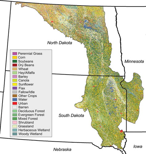
The study area is the Northern Glaciated Plains ecoregion (US EPA 1999) covering approximately 141,000 km² (Figure 1). Historically the region was primarily grassland, but today agricultural land uses cover most the ecoregion (over 65%) and only ~16% of the ecoregion remains in grassland (US Department of Agriculture, 2012a). Of land used for cropland, over two-thirds is used for corn or soybean production, and these two crop classes are particularly dominant in the southern and eastern portions of the ecoregion. Wheat and canola are prevalent in many northern portions the ecoregion, while various small grains, dry beans, alfalfa, and other crops are locally important. Water and wetland covers over 10% of the ecoregion area, with relative proportions between the two often fluctuating due to short-term weather and climate variability. Developed lands cover only about 3% of the landscape, with Sioux Falls, South Dakota, representing the largest urban center in the ecoregion with a population of over 150,000.

Figure 1. Northern glaciated plains ecoregion, with starting 2012 land cover from the cropland data layer. The region covers over 140,000 km² and 956,983 individual ownership/management units.

2.2. LULC and parcel data

The US Department of Agriculture (USDA) Cropland Data Layer (CDL) data was used as the starting LULC (USDA 2012a). CDL data is a remote sensing-based LULC product that provides detailed, spatially explicit information on crop types for the conterminous United States, with a spatial resolution of 30 m. The 2012 version of the CDL was used to represent initial LULC for this application as 2012 represented the initial date for the scenario we modeled (as described below). Ten crop classes covered more than 400 km² in the ecoregion: these crops were maintained as unique classes in the final classification scheme, while all other crops were lumped into a generic ‘other cropland’ class. Non-cropland classes in the 2012 data set were maintained as individual classes for modeling, with the exception that the four urban/developed classes were aggregated into a single urban/developed class. The final thematic classification scheme used for this work is shown in Figure 2.

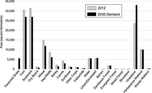
Figure 2. Starting LULC proportions for 2012, and the targeted proportions for 2030 based on the Billion Ton Update scenario.

Parcel data representing agricultural ownership and management boundaries came from the USDA Common Land Unit (CLU) data set, a program established to provide a digital records database for the administration of agricultural, conservation, and disaster programs (USDA 2001, 2012b). CLU data consists of vector-based boundaries that delineate contiguous regions of common land ownership, management, and land cover characteristics, with boundary delineation corresponding to features such as roads, fence lines, property boundaries, water features, or other easily identifiable features that separate ownership and management units. Due to concerns about confidentiality and privacy of individual land owners, these data were no longer publicly available after the 2008 Farm Bill was enacted. However, circa 2008 CLU data that were downloaded and used for prior work were available for the study area. These unattributed circa 2008 parcel boundaries were used to define ‘current’ agricultural fields for this application. Any parcel changes that may have occurred between 2008 and 2012 were thus not reflected in our starting 2012 date.

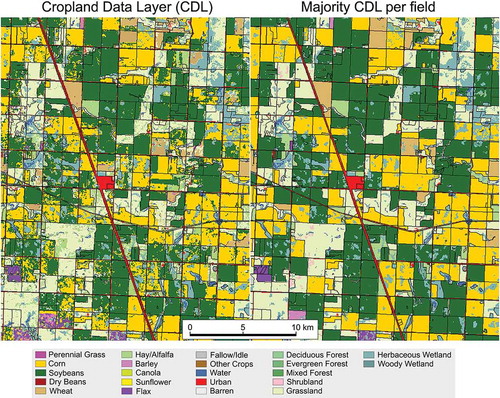
The CLU boundaries were used within a modified FORE-SCE model to represent parcel-level change for cropland areas, but the model itself remained raster based. CLU polygons were rasterized to 30-m pixels, with all pixels that fall within an individual field given a unique field ID. There were 956,983 individual parcel units within the study area, with a mean parcel size of ~16 ha (median parcel size ~4.2 ha). Each parcel was treated as a homogenous and discrete LULC unit, particularly for agricultural land uses, but an overlay of the CLU boundaries on the 2012 CDL data revealed that many individual fields contained scattered pixels of multiple crop classes. A majority filter was used to assign all pixels within a CLU parcel to the CDL cropland class that represented a majority of that field (Figure 3). Within an individual CLU field, the CDL may also include small patches of wetland or forest. Examination of aerial photography indicates that many of these represented real patches of wetland or treed land cover within an agricultural field, but some likely represented classification error in the original CDL data. Regardless of the source, if pixels of a non-cropland class were found within a CLU parcel, these pixels were maintained as the native LULC class from CDL. Filtering altered total cropland proportions slightly from the original CDL data, but nearly all crop classes were within 5% of the original CDL total. The exception was the aggregated hay/alfalfa class, where filtering resulted in a 13% reduction from the original CDL total. This was primarily due to the elimination of scattered hay pixels found throughout cropland classes in the original CDL. The modified version of the 2012 CDL represented our starting LULC data set.

Figure 3. The crop type (from CDL) that composed the majority of a given field (from CLU) was assigned to all agricultural pixels within that field. Water, wetland, and urban pixels within a given field were maintained.

2.3. Modeling framework

A modified version of the FORE-SCE model was used for this application. The original model is fully described in Sohl et al. (2012, 2014). Many components mimic past FORE-SCE applications, but substantial modifications were made to FORE-SCE to enable parcel-based, high-resolution modeling. FORE-SCE’s general structure handles issues of scale by linking demand and spatial allocation components. Demand for FORE-SCE can potentially take multiple forms, but in general provides a ‘prescription’ for overall LULC change across a broad geographic region. Past applications have most frequently used a matrix form of demand, where economic models, historical trend extrapolations, or cooperative scenario construction workshops were used to provide complete, aggregate ‘from-to’ change matrices for future LULC change across a broad region (Sleeter et al., 2012; Sohl et al., 2014, 2012). FORE-SCE can also use a different algorithm for incorporating demand, using a simpler proportional demand format that simply defines aggregate-level LULC proportions for future dates. For a FORE-SCE application using proportional demand, the exact ‘from-to’ transitions are derived within the spatial allocation module itself. For this application, proportional demand was used to provide aggregate LULC change across the Northern Glaciated Plains ecoregion from 2012 to 2030.

The spatial allocation component of FORE-SCE uses demand as a prescription for regional LULC change and produces a spatially explicit map. At the core of all FORE-SCE spatial allocation methodologies are suitability surfaces, spatial representations of site-specific capability of the landscape to support a given LULC class (Sohl et al., 2016, 2014). FORE-SCE has multiple options for placing change on the landscape, guided by the individual suitability surfaces for each LULC class. In all options, change is placed on the landscape one patch or parcel at a time. The suitability surfaces guide the placement of ‘seed’ pixels dictating where a new patch of LULC change is prescribed to occur, with a ‘clumpiness’ parameter used to control how clumped or dispersed newly placed LULC change is for a given LULC class (Sohl et al., 2014). Past FORE-SCE applications used a patch-growing algorithm (Sohl et al. 2007) or a patch-library approach (Sohl et al., 2014, 2012) to place a patch of change on the landscape, centered on a placed seed pixel. The number of patches that are placed on the landscape for each modeled LULC class is dependent upon prescribed quantities from demand. While these approaches have been effective at mimicking realistic patch sizes for a given region (using historical data to parameterize patch characteristics), older placement procedures ignore ownership- and management-based parcels and existing patch boundaries. For this application, the CLU field boundaries were used to spatially constrain the placement of change, with agricultural change modeled field-by-field. The following summarize the demand and spatial allocation components for this application.

2.3.1. Demand and the BTU

Quantitative demand across the Northern Glaciated Plains was provided by a scenario from the US Department of Energy’s BTU (US DOE 2011). The BTU is a follow on to the Billion Ton Study (Perlack et al., 2005), an examination of the feasibility of producing 1 billion tons of biofuel feedstock annually in the conterminous United States. The BTU improved upon the Billion Ton Study using economic and policy modeling to estimate county-level production of major crops, including food crops, and traditional biofuel crops such as corn and soybeans. The potential development of a cellulosic-based biofuel industry was also represented in the BTU by including perennial grasses and woody crops. An advantage to using BTU scenarios for agricultural projections is that the data provide (1) county-level estimates of agricultural change, facilitating a spatial comparison of model performance against the scenario source, and (2) individual projections for major crop classes, including a ‘perennial grass’ class designed to represent feedstocks for cellulosic ethanol production. One scenario from the BTU was selected for modeling, a ‘high-yield’ scenario with an assumed $80 per ton farmgate price for dry biomass feedstock, and a 4% annual yield increase assumption. This specific BTU scenario was selected because it projected very high levels of cropland change, and thus was a good test of model performance in a dynamic agricultural setting. Under this scenario, overall cropland in the ecoregion declines substantially from 2012 to 2030, particularly for traditional crops in the region such as corn, soybeans, and wheat. However, the scenario assumes a strong demand for cellulosic biofuel feedstock, and thus projects a very large expansion in the cultivation of a ‘perennial grass’ class.

Given the large number of counties within the ecoregion and spatial and quantitative mismatches between the BTU scenario and our starting 2012 CDL, it was not practical to individually parameterize and model each county individually. County-level estimates from the BTU scenario were aggregated for the Northern Glaciated Plains ecoregion to develop demand for the years 2012–2030. The BTU is thus serving to provide the overall broad regional scenario based on generalized economic and policy variables, while FORE-SCE is being used to provide a spatially explicit representation of the broad scenario using parcel-level agricultural fields and a statistical characterization of the landscape’s suitability to support each modeled LULC class. The BTU county-level estimates for 2012–2030 include changes in corn, soybeans, wheat, hay, sorghum, barley, oats, and perennial grasses, covering most of the major cropland classes in this ecoregion. Given the mismatches between the 2012 BTU and the 2012 CDL (disagreement in county-level proportions of individual crop types), percent change values from the BTU were applied to starting 2012 CDL LULC proportions to derive a prescription for 2012–2030 change. Projected quantitative changes for the crops that were not included in the BTU data including canola, flax, sunflower, and dry beans were determined by applying overall rates of BTU-defined agricultural cropland change in the ecoregion from 2012 to 2030 (decline of approximately 8%). Demand for urban area (~8% increase from 2012 to 2030) was obtained from the IPCC SRES A1B, as modeled with an earlier FORE-SCE application for the conterminous United States (Sohl et al., 2014). With the desire to focus on changes in agricultural and urban land, most natural LULC classes (grassland, shrubland, the three forest classes, and the two wetland classes) were ‘passively modeled’ by FORE-SCE. For these classes, no direct demand was specified in the model, but substantial changes could occur due to corresponding changes in the actively modeled cropland and urban classes. For example, the BTU scenario projects a very strong decline in agricultural land overall for the counties in this ecoregion. In an ecoregion where grassland is the predominant ‘natural’ LULC class, agricultural land that is abandoned most frequently reverts to the native grassland state. Thus as parcels of cropland are abandoned between 2012 and 2030, a subsequent increase in passively modeled grassland occurs. Figure 2 provides a summary of both the starting 2012 LULC and the 2030 target proportions of each LULC class. Note that while FORE-SCE can model yearly iterations (or any other desired time step), for this application, only a single time step was modeled, directly from 2012 to 2030.

2.3.2. Spatial allocation in FORE-SCE

The development of suitability surfaces used to guide the allocation of LULC change was based on statistical relationships between the starting 2012 CDL and ancillary data sets that may help predict where a given LULC class is likely to occur. Sample points were randomly selected from across the study area (typically many hundreds per LULC class). Logistic regression was used to derive the probability of occurrence/non-occurrence for each LULC class at a pixel level, resulting in spatially explicit suitability maps that were generated for each modeled LULC class. For this application, much of the focus was on the modeling of agricultural lands. Factors that drive site-specific suitability for agricultural land use include terrain, climate, soil properties, and socioeconomic factors (Baker & Capel, 2011). These and other variables were used as independent variables in the creation of suitability surfaces for each modeled LULC class (Table 1). Suitability surfaces were first established for the starting 2012 date. Suitability surfaces for 2030 were generated using regression coefficients established for the 2012 date, but with substituted 2030 climate data from WorldClim (WorldClim, 2015), thus representing potential shifts in suitability due to projected climate change.

Table 1. Ancillary data sets used in the construction of suitability surfaces for the spatial allocation component of FORE-SCE.

Data set	Description	Data source
Topographic
Elevation	Elevation in meters	National Elevation Database^1
Slope	Slope in degree	National Elevation Database^1
CTI	Compound topographic index	National Elevation Database^1
Soils
Root zone H2O	Root zone available water storage	SSURGO^2
Crop productivity	National commodity crop productivity	SSURGO^2
Hydric soils	Hydric rating (percent)	SSURGO^2, STATSGO^3
SOC	Soil organic carbon for top 100 cm	SSURGO^2, STATSGO^3
Census/demographics
Pop. density	Population density	TIGER/LINE block level^4
Housing density	Housing density (total households)	TIGER/LINE block level^4
Climate
Fall Tmax	Fall (September, October) mean maximum temperature	WorldClim, 30-s climate data^5
Spring Tmax	Spring (March, April) mean maximum temperature	WorldClim, 30-s climate data^5
Late summer Tmin	July, August mean minimum temperature	WorldClim, 30-s climate data^5
Spring precip.	Spring (March, April) total precipitation	WorldClim, 30-s climate data^5
Growing season precip.	Growing season (May–September) total precipitation	WorldClim, 30-s climate data^5
GDD	Growing degree days	WorldClim, 30-s climate data^5
Proximity
Road distance	Distance from 2012 primary and secondary roads	2012 TIGER roads shapefile^6
Rail distance	Distance from 2012 rail lines	2012 TIGER national rails shapefile^6
Water distance	Distance from surface water	2014 National Atlas hydrography data^7
City distance	Distance from 2012 urban area	2012 TIGER urban area shapefile^6

¹Gesch, 2007

²USDA-NRCS 2015

³USDA-SCS 1993

⁴US Census Bureau, 2015a

⁵WorldClim, 2015

⁶US Census Bureau, 2015b

⁷USGS 2015

A new version of FORE-SCE that uses field boundaries to represent parcel-level change was developed. Suitability surfaces still dictated the likelihood that a given parcel of land can support a given LULC class, and the overall modeling process remained raster-based. However, a rasterized parcel index image, where each parcel in the ecoregion has a unique ID, was used to spatially constrain modeled LULC change. When a new parcel of a given LULC change was required, a seed was placed on the suitability surface as with past FORE-SCE applications. The seed location was then intersected with the parcel index image, and all pixels associated with that field were flagged. The new LULC class was applied to all pixels within the field, and the process moved to the next seed and parcel. Field parcels were thus respected and entire agricultural fields were changed to ‘new’ LULC classes at one time. To better represent landscape pattern, we used a much finer spatial resolution (30 m pixels) compared to past FORE-SCE versions (250 m pixels). In older FORE-SCE applications, the 250 m pixel size was near or even larger than the mean historical patch size of change for a given LULC transition, leaving the model incapable of spatially representing fine-scale change. The use of a 30-m pixel enabled us to (1) represent smaller agricultural parcels, (2) represent field shape using multiple individual pixels within a raster-based framework, and (3) maintain consistency with many LULC databases for the United States such as NLCD (Fry et al. 2011), LANDFIRE (Rollins, 2009), or the CDL used as the starting LULC in this assessment (US Department of Agriculture, 2012a).

The new parcel-level allocation process was used in this application to represent all LULC transitions involving cropland classes. However, while cropland change does typically occur field-by-field, for some LULC classes, older FORE-SCE allocation methods may be preferable. For example, urban changes typically occur as aggregates of small patches of change, representing the construction of individual developments, or even individual houses, businesses, and industrial units. Using CLU parcels to represent urban change, changing entire parcels at one time, is less realistic than it is for modeling agricultural change. For this modeling application, we thus used FORE-SCE’s ‘patch grow’ allocation methodology to represent urban change. A seed was placed on a location likely to support new urban lands, and a patch organically ‘grows’ from the seed pixel location, based on the underlying suitability surface characteristics (e.g. ‘growing’ into highly suitable areas while avoiding unsuitable areas). As with past FORE-SCE applications, once an urban seed was placed, a distribution of historical urban patch sizes was consulted, with a stochastic algorithm used to assign a realistic patch size based on regional historical LULC data. Patch sizes in the model were parameterized with data from the USGS Land Cover Trends project (Loveland et al., 2002).

Patches were placed on the landscape one at a time, until demand was met for a given LULC class, with processing then continuing to the next LULC class. After the initial allocation, it is unlikely that overall LULC proportions match demand, as net change resulting from class-by-class allocation must be resolved. An automated iterative process was used within FORE-SCE to resolve competition between all classes and balance LULC proportions to match demand. After the initial allocation, the number of patches for each LULC class was adjusted as follows:

where x = iteration number; y = LULC class; NewPatch_x+1,y = number of allocated patches for model iteration x + 1 for LULC class y; OldPatch_x,y = number of allocated patches used in model iteration x for LULC class y; Demand_x,y = prescribed demand (area) for LULC class y in iteration x; and Allocated_x,y = actual area allocated for LULC class y in iteration x.

Simply put, if a given LULC class was underallocated for the initial iteration, the number of new patches added for that class was adjusted upwards, while the number of patches was reduced for classes that are overallocated. The process repeated over multiple iterations, with iterations continuing until (1) overall LULC proportions ‘settled down’ and were all within a predefined tolerance from demand or (2) a predefined number of iterations were completed. For this application, we specified a tolerance level of ±1% from demand for each modeled LULC class or a maximum of 20 iterations.

With FORE-SCE’s proportional demand allocation, what LULC class a new patch ‘comes from’ is primarily dependent upon the intersection of the suitability surface for the new LULC class and the existing LULC. For example, if demand prescribes an increase in the area of cropland used for ‘corn’, new fields will be allocated in areas deemed to be highly likely on the suitability surface for corn. The non-corn LULC class(es) that most often intersect high probability values for corn were most likely to be selected and changed by the prescribed increase in corn. FORE-SCE also uses an elasticity modifier to control the likelihood of a given LULC transition. Based on the history of a given region, or based on the desired scenario or storyline, elasticity values can be used to tightly control the types of LULC transitions that occur. An elasticity matrix is populated for each possible LULC transition, with elasticity values ranging from 0 to 1. These are simple multiplicative modifiers to overall suitability values, applied at the start of the spatial allocation process. Values of ‘0’ effectively eliminate the possibility of a given LULC transition, while values of ‘1’ offer no adjustment to baseline suitability values. For this application, elasticity modifiers were used to eliminate the possibility of urban lands transitioning to other LULC classes in the future and to provide increased control on cropland conversions. For example, transitions between crop types were freely allowed, with no elasticity modification to reduce the likelihood of a given crop-to-crop transition. However, elasticity was used to reduce the likelihood that wetland or forest classes would transition to crop classes. In effect, elasticity settings ensured most cropland increases specified by the BTU scenario came from (1) other cropland or hay classes or (2) existing grassland.

2.3.3. Modeling uncertainty assessment and Monte Carlo runs

Past applications of FORE-SCE have been assessed by comparing model results to historical reference data sources, most extensively for a modeled historical ‘backcast’ land cover from 1938 to 1992 for the conterminous United States (Sohl et al., 2016). However, no formal validation of model runs against a historical reference database was performed for this application. The lone BTU scenario is but one potential realization of the future landscape, and the scenario approach used here is by itself not subject to an assessment of uncertainty or validation. However, we can assess FORE-SCE itself in terms of (1) how well the model matched overall proportions of LULC change prescribed by the BTU scenario and (2) how well the modeled data matched BTU spatially at the county level. Both are discussed in Section 3.

Past FORE-SCE applications produced but a single realization of a given modeled scenario. With this application, we produced a probability-based representation of the BTU scenario as modeled by FORE-SCE using a Monte Carlo approach. Fifty individual model runs were completed, with stochastic variation of model parameters to assess uncertainties introduced by FORE-SCE itself. The suitability surfaces created for each LULC class played a vital role in determining the spatial distribution of mapped LULC change in FORE-SCE, yet the underlying logistic regression used to create suitability surfaces was subject to statistical uncertainties. For each of the 50 Monte Carlo runs, regression coefficients for each suitability surface were stochastically altered based on coefficient standard errors. Other FORE-SCE variables such as the aforementioned ‘clumpiness’ variable were also stochastically altered (around standard mean values) for each model run. The model has the capability to also utilize different Global Climate Model (GCM) realizations of a given climate scenario to account for uncertainties between GCMs. However, given the relatively short modeling time used here (2012–2030), we only used one future climate data set representing mean conditions across multiple models and scenarios. Data from the Community Climate System Model (Gent et al., 2011) and Goddard Institute for Space Studies E2-R model (Schmidt et al., 2014) were averaged across each of the four IPCC Representative Concentration Pathways scenarios. The Monte Carlo runs and the resultant, aggregate probability-based maps thus represent uncertainty in FORE-SCE’s portrayal of the modeled BTU scenario due to stochasticity of model parameters and the statistical representation of the probability surfaces, but do not include uncertainty due to climate scenarios or the use of different GCMs.

2.3.4. Comparison of parcel-based model with past FORE-SCE modeling

To assess the impacts of both spatial resolution differences in the models and parcel versus pixel-based modeling, comparisons were made among the following five data sets:

1. Starting 2012 land cover, at 30-m resolution

2. Starting 2012 land cover, at 250-m resolution

3. 2030 modeled land cover, at 30-m resolution, using new parcel-based model

4. 2030 modeled land cover, at 30-m resolution, using old pixel-based model

5. 2030 modeled land cover, at 250-m resolution, using old pixel-based model

Note there was no 250-m parcel-based model run as the frequency of parcels smaller than the 250-m pixel size made such a run impractical. The same scenario input was used for each of the three 2030 model runs.

Regardless of the FORE-SCE model version, the prescribed quantity of LULC change from the scenario (‘demand’) is met quite well; the best indication of differences in model performance is thus the spatial allocation of the prescribed change. To assess the impact of spatial resolution, and parcel- versus pixel-based modeling, select landscape metrics were calculated and compared for the five data sets listed above. Landscape metrics were calculated across the entire study area using Fragstats 4.2 (McGarigal, Cushman, & Ene, 2012). Four individual metrics were calculated for each modeled LULC class, including (1) number of patches, (2) total edge, (3) mean patch size, and (4) shape index. Description of the individual metrics may be found in McGarigal (2015).

3. Results

3.1. Modeled FORE-SCE output

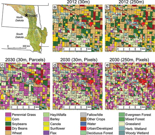
We produced 50 model realizations of the BTU scenario, as well as aggregate probability-based representations for each modeled LULC class. Figure 4 represents an example of modeled LULC for a small part of the ecoregion in central North Dakota, including (1) the starting LULC in 2012 at both 30- and 250-m resolutions (panels A and B, respectively), (2) 2030 LULC from the new, parcel-based model at 30-m resolution (panel C), and (3) 2030 LULC from the older, pixel-based model at both 30- and 250-m resolutions (panels D and E, respectively). The modeled BTU scenario calls for a large increase in perennial grass (used as a cellulosic biofuel feedstock), with the clear majority of it occurring in the far western counties of the ecoregion. The region shown in Figure 4 was chosen to represent model performance in a high-change area, with many parcels transitioning to perennial grass between 2012 and 2030. Grassland increases by over 40% by 2030 (Figure 2), with most of the increase resulting from cropland conversion to grassland (as shown in Figure 4). While overall proportions of LULC change are the same between the parcel-based model and the older pixel-based model, clear differences are obvious in spatial patterns. The older, pixel-based model produces a much more fragmented looking landscape at both the 30- and 250-m resolutions, with greater variability in patch size and new patches of LULC change that clearly cross existing field boundaries.

Figure 4. A final model run for a portion of the ecoregion in central North Dakota. The five panels represent starting land cover in 2012 (both 30-m (A) and 250-m (B) resolution), the new parcel-based, 30-m resolution model for 2030 (C), the old, pixel-based, 30-m resolution model for 2030 (D), and the old, pixel-based, 250-m resolution model for 2030 (E).

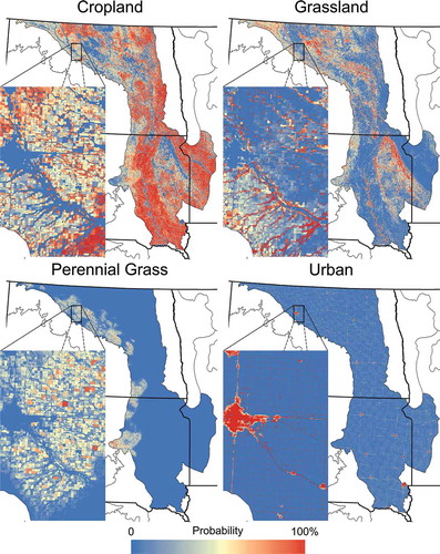
Figure 5 depicts aggregate probabilities across the 50 Monte Carlo runs for the year 2030. It was the interplay between (1) the large increase in perennial grass, (2) the overall decline in cultivated crops, (3) the resultant increase in natural grassland, and (4) the increase in urban area that drove overall change in the scenario: thus, these are the four classes depicted in Figure 5. Select ‘core’ areas of cultivated crop are present in most model realizations, including large areas in the southern and eastern parts of the ecoregion. More uncertain areas are found where cultivated cropland competes with perennial grass and natural grassland, with uncertainty driven in part by the stochasticity of which exact farm field is targeted for change in each Monte Carlo run. This is particularly evident in the western part of the ecoregion, where new broad-scale perennial grass cultivation occurs, and in scattered areas such as the Prairie Coteau, the wedge-shaped plateau in the southeastern part of the ecoregion where grassland and wetland compete with cultivated cropland. Of all LULC classes in Figure 5, urban areas exhibit the least variability among model runs as new urban lands are always concentrated around existing urban centers and road networks.

Figure 5. Aggregated probability-of-occurrence for the year 2030 across 50 Monte Carlo runs for (1) cropland (aggregate of all cultivated crop classes), (2) natural grassland, (3) perennial grass (biofuel feedstock under the BTU scenario), and (4) urban lands.

3.2. Matching BTU demand

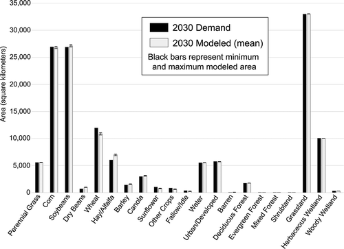
Figure 6 summarizes modeled results for overall proportions of LULC, including minimum, maximum, and mean values across the 50 Monte Carlo runs for each LULC class and a comparison with the prescribed demand from the BTU scenario. Prescribed demand was unchanged among all 50 Monte Carlo runs, but stochastic elements that drove where change patches were placed by FORE-SCE resulted in both quantitative and spatial differences between Monte Carlo runs. Quantitative differences in LULC proportions were generally small as FORE-SCE was able to match BTU scenario demand well overall for all Monte Carlo runs. Unlike past versions of FORE-SCE that used a matrix form of demand (Sohl et al., 2016, 2014), the quantitative match between demand and model results is not exact, however. With the proportional demand allocation methodology, individual transition types are less tightly controlled, and the iterative process to balance net change between LULC classes may not be able to exactly match prescribed demand. The underlying suitability surfaces strongly control the LULC transitions that occur as the model attempts to match demand, and in some cases, a form of ‘mismatch’ occurs between the suitability surfaces and demand. For example, while most LULC classes matched demand very closely, wheat declined more than expected (−2,792 km² demand, −3,876 km² model mean), while hay declined less than expected (−2,407 km² demand, −1,459 km² model mean). FORE-SCE closely matched prescribed demand for the three classes that substantially increased from 2012 to 2030 (urban, perennial grass, and natural grassland), while overall matches were less exact for LULC classes that declined.

Figure 6. Modeled results compared to BTU scenario demand for 2030. Model means for each LULC class are shown, along with minimum and maximum area modeled across the 50 Monte Carlo runs.

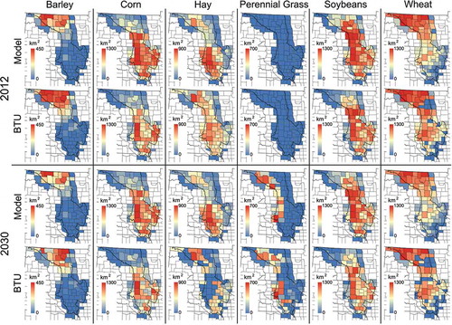
Figure 7 depicts county-level spatial patterns for both the BTU scenario and (mean) model results, for 2012 and 2030, for each of the six major crop classes directly modeled for the BTU. Spatial patterns at the start of the simulation period in 2012 were similar for most of the classes, but substantial differences exist at a county level. Modeled change to 2030 also shows similar patterns to the 2030 BTU data, but with some differences at a county level. Given the differences between the BTU data and our starting 2012 CDL, before modeling begins, it is difficult to attribute differences in spatial pattern in 2030 to the modeling itself, or to the original source data differences.

Figure 7. County-level comparison between modeled and BTU data, depicting quantity of six major cropland classes. For counties that intersect the border of the modeled ecoregion, BTU crop areas were adjusted proportionally according to the area of the county within the ecoregion boundary.

3.3. Comparison with non-parcel version of FORE-SCE

Figure 8 compares landscape metrics for the five most common land covers from (1) the starting 2012 land cover (both 30- and 250-m resolutions) and (2) from the three 2030 models (the new parcel-based model at 30 m and the older FORE-SCE model at both 30- and 250-m resolution). Some of the metric differences were attributable to spatial resolution effects, given the substantial differences in individual class metrics before modeling begins in 2012. However, trends in landscape metrics from 2010 to 2030 reveal substantial differences between the pixel- and parcel-based approaches.

Figure 8. Landscape metrics for the five most common land cover classes for (1) the starting 2012 land cover at both 30- and 250-m resolutions and (2) the modeled 2030 land cover from the new 30-m parcel-based model, and from the old pixel-based model at both 30- and 250-m resolution.

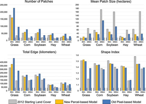
Grassland represented the underlying, native landscape ‘base’ on which most agricultural activity occurred in the ecoregion. Grassland increased by over 40% from 2012 to 2030 (Figure 2). For the new parcel-based model (30-m resolution), the number of patches declines and mean patch size increases as grassland gains result in a coalescing of individual grassland patches into fewer, larger patches. Despite the decline in grassland patch number, total edge increases due to the much larger extent of grassland overall. For the older pixel-based model at the same 30-m resolution, trends in landscape metrics are dramatically different. Fragmentation of the grassland mosaic increases substantially compared to the parcel-based model, with an increase in the number of patches, a much smaller patch size increase (despite the larger increase in grassland overall), and a drastic increase in total edge. Increased fragmentation is also evident in the 250-m, pixel-based model, with large increases in the number of patches and total edge, and a decrease in mean patch size. Shape index values for grassland show only minor change from 2012 to 2030 in the 30-m models, but increase sharply for the 250-m, pixel-based model.

2012–2030 trends are similar for the four crop classes in Figure 8. In the 30-m parcel-based model, the number of cropland patches generally increases while both total edge and mean patch size decrease. While counterintuitive in a scenario where cropland declines in area, the patterns are a result of large, contiguous blocks of individual farm fields becoming increasingly fragmented as individual cropland fields convert to grassland or perennial grass. The fragmentation is substantially more severe for both the 30- and 250-m pixel-based models, with much higher increases in the number of patches, an actual increase in total edge (despite significant cropland area loss), and a stronger reduction in patch size.

4. Discussion

Moving to a parcel-based modeling approach has strong impacts on the representation of landscape pattern. Landscape metrics results make it clear that the newer, parcel-based approach led to a projected landscape with characteristics more like current landscape patterns, while the older approach produced more irregular, fragmented landscape patterns. In models that ignore existing ownership and management parcels, new patches of LULC change are inevitably placed in locations that cross existing field boundaries, resulting in an artificial fragmentation of the landscape. This results in trends in landscape metrics over time that not only may differ in magnitude between the parcel- and pixel-based models, but may even differ in direction (e.g. a decline in number of grassland patches in the parcel-based model versus a large increase in grassland patches for the pixel-based model).

Our ability to realistically portray both the diversity and spatial pattern of many different land cover classes, including cropland type, greatly facilitates the use of these projections for ecological assessments. For example, assessments of vertebrate and invertebrate biodiversity in agricultural settings are highly sensitive to landscape pattern (Duflot, Aviron, Ernoult, Fahrig, & Burel, 2015). Realistic representation of agricultural landscape patterns is also important for assessments of water quality and other hydrological processes (Bu, Meng, Zhang, & Wan, 2014; Gonzales-Inca, Kaliola, Kirkkala, & Lepisto, 2015). An additional advantage of the new modeling approach is the ability to track individual parcels over time from the assigned unique ID for each field. This enables the attribution of fields with information that can be used within the modeling framework itself. For example, field ID’s can potentially be used to represent realistic crop rotations. Current work is focused on the use of crop rotation data (Osteen, Gottlieb, & Vasavada 2012) to mimic realistic crop rotation patterns. Cross-referencing field IDs with FORE-SCE’s ‘history’ variable (recording the history of LULC change for a pixel) enables the probabilistic modeling of annual crop maps, with field-by-field crop rotation that mimics historical patterns. Such an approach further expands FORE-SCE’s capabilities to support LULC change impact assessments, given that crop rotation and management has a strong effect on soil biogeochemistry and other processes (Havlin, Kissel, Maddux, Claassen, & Long, 1990).

FORE-SCE itself showed an ability to match the general characteristics of the BTU scenario, but there were some noted differences in both the overall proportions of LULC change (Figure 6) and in terms of the county-level spatial pattern (Figure 7). The largest proportional differences were with the wheat and hay classes, with too much wheat and too little hay removed by 2030 when compared to the BTU scenario. These differences are primarily due to the characteristics of the perennial grass probability surface used by FORE-SCE. Few fields in the ecoregion are currently being planted in perennial grasses, leading to a sparse sample for construction of the perennial grass suitability surface. Suitability surface characteristics were thus somewhat mismatched with county-level perennial grass estimates from the BTU scenario. As a result, FORE-SCE placed more perennial grass in select northern counties and less in some west-central counties compared to the BTU scenario. The northern counties had less hay and more wheat relative to the west-central counties; thus FORE-SCE allocated more ‘wheat-to-perennial grass’ and fewer ‘hay-to-perennial grass’ transitions than might be expected from the BTU scenario. Figure 7 also shows counties in multiple crop classes that ‘zero out’ by 2030 in the BTU scenario, with no such decline in the FORE-SCE results. For example, many counties in the west-central part of the ecoregion have high levels of hay in 2012, but drop to zero hay pixels by 2015 or 2020 in the original BTU scenario. The FORE-SCE depiction of the scenario showed more gradual change, often spread across a wider geographic area. Discrepancies among the original source LULC data set also drove some of the disagreement between the original BTU scenario and the FORE-SCE modeled scenario. From the start of the simulation in 2012, there were quantitative and spatial pattern differences between our starting 2012 CDL data and the county-level BTU scenario data. Such differences affected the modeling results themselves, as well as our ability to attribute the causes of any differences with modeled results versus the 2030 BTU results.

Acquisition of suitable parcel boundary data is likely a limiting factor for using this methodology for some applications. Past model applications highlight the difficulty in acquiring field boundaries based on ownership and land management. Brown and Castellazzi (2014) noted confidentiality restrictions on the use of the parcel-level data they used for Scotland, while Berger and Bolte (2004) were forced to use a combination of Oregon Water Resources Department ‘irrigation place-of-use’ parcel data along with manually digitized field boundaries from remote sensing imagery. Modeling at the parcel level across broad geographic regions has rarely been attempted, partially because ownership- and management-based parcel data is typically only available for small regions (Radeloff et al., 2012). The CLU data used here to delineate agricultural fields facilitates the modeling of agricultural land parcels at broad scales, but the data is no longer publicly available, particularly boundary data complete with detailed attributes collected by the USDA. Older versions of unattributed vector data are currently available for some locations from multiple online sources, but there is no guarantee this will continue into the future. It is also recognized that data similar to CLU is likely not available for many locations outside of the conterminous US. Parcel-based spatial data is also much less likely to be available for some land use sectors than others. This includes intensively managed forest areas in the United States, where the treatment of trees as a crop results in extensive, often temporally frequent, land cover changes.

However, alternatives to rigorously collected and maintained land management and ownership parcels across broad areas, such as the CLU data, are starting to become available from the remote sensing community. Yan and Roy (2014, 2016) recently developed a technique to extract contiguous agricultural management units from historical Landsat series, with resultant field boundaries that are somewhat comparable to CLU data for agricultural lands. However, the Yan and Roy data are much less complete than CLU data, only providing field boundaries for fields actively being used for cropland at the time of satellite observation. Such a data set is potentially useful when modeling future scenarios where cropland extent is stable or declining, but for scenarios of future cropland expansion, there is an inadequate representation of current non-cropland parcels. Thus, there are no non-cropland parcels for new cropland to appear. Parcel-based data would also be extremely useful for the modeling of forest management and change, yet ownership- and land management-boundaries for forested lands are even less likely to be available than for agricultural lands. In lieu of the availability of large-area, high-resolution parcel data for forested regions, Butler, Hewes, Liknes, Nelson, and Snyder (2014) used a modeling approach to approximate large-area ownership patterns for several US states, but these data were much coarser than the resolution of a data set such as CLU. Widespread adoption of parcel-based, broad area LULC modeling will continue to be hobbled without increased availability of actual cadastral-based ownership data or improvements in the availability of remote sensing-based land management parcels.

We also note several caveats for this specific application. With a focus on aggressive biofuel production, including cellulosic-based biofuel, the original BTU scenario included a cultivated ‘woody biomass’ class. For the Northern Glaciated Plains ecoregion, several northeastern counties were projected to have large increases in woody biomass. Given the history of the region as highly productive cropland, this was deemed to be unrealistic, and woody biomass was not modeled. Given our focus on modeling parcel-level cropland change, we also did not model any potential changes between ‘natural’ LULC classes such as forest, wetland, and grassland. FORE-SCE’s dynamic suitability surfaces were able to capture changes in suitability as climate changed between 2012 and 2030, but with a relatively short time frame, impacts of climate on the results were muted. The 2030 climate data also included modest novel conditions outside the range of the training data used in the 2012 logistic regressions. We also did not account for potential feedbacks between climate change, water availability, and agricultural land use, including potential impacts on irrigated agriculture. Finally, for this proof-of-concept application where a single modeled time step was used, we did not capture gross change that would occur over the 2012–2030 time step, including the effects of crop rotation.

Finally, we note that spatially explicit LULC models in general have tended be geostatistical models driven by remote sensing or other spatially explicit data. While these approaches can be effective at representing landscape pattern, they are generally poor at explaining underlying LULC change processes and driving forces. Process-based LULC models are needed to better represent the decision-making processes that drive actual land use at a local scale (National Research Council, 2013). However, it is simply not feasible to model individual land owner decisions for the nearly 1 million agricultural parcels found in a broad geographic region such as the Northern Glaciated Plains. The field boundaries we used to guide the spatial allocation of change may represent ‘real’ land management units, but without linkage to ownership information, it is impossible to represent the unique driving forces on which each landowner bases their decisions, or to represent landowner decisions in aggregate across each of their individual fields. The approach described here certainly cannot be categorized as a process-based or agent-based model, with the spatial allocation algorithm used by FORE-SCE still clearly falling into the category of an empirically driven geostatistical model. With such a geostatistical approach, we are modeling the outcome of human behavior, rather than modeling the behavior itself (Irwin & Geoghegan, 2001) as would an agent-based model. However, when we combine high-resolution, spatially explicit parcel data, a practical broad-area spatial allocation algorithm, and an exogenous economic scenario that explains aggregate landowner response to policy and economic driving forces, it enables us to mimic aggregate land ownership decisions. While the allocation component remains an empirical/statistical model, this approach improves upon existing models and better represents local and aggregate landscape patterns resulting from individual land owner decisions under macro-scale driving force scenarios.

5. Conclusions

To our knowledge, no spatially explicit LULC modeling application to date has modeled agricultural land use using parcels based on true ownership and management boundaries for such a broad geographic region. The application of the parcel-based FORE-SCE model to the Northern Glaciated Plains ecoregions covered over 140,000 km² and nearly 1 million individual agricultural fields. Parcel-based LULC models and LULC models in general also tend to focus on narrow thematic LULC classes (e.g. urban modeling or parcel-based modeling of agricultural crops in aggregate). This application provided detailed crop-specific mapping across a broad-geographic region, while also including a wide variety of other primary LULC classes. This application also included potential effects of climate change on site-level suitability for a given LULC class, something not generally incorporated in parcel-level modeling.

The structure of LULC models generally becomes more complex when parcel-level modeling is used instead of square pixels (National Research Council, 2013). However, the framework used here, linking existing quantitative, economics-based, regional LULC scenarios with a highly detailed spatial modeling algorithm, is practical and generalizable, offering the potential to provide similar parcel-based LULC projections for other geographic regions. Through aggregation of multiple state or ecoregion-level modeling applications, it certainly is feasible to do national-scale LULC projections for the United States, replicating the spatially explicit, national-scale LULC projections completed by Sohl et al. (2014) and Sohl et al. (2016) but at much higher spatial and thematic resolutions, with parcel modeling ensuring a vastly improved representation of local landscape pattern. Availability of consistent, broad-scale parcel data is likely the biggest practical constraint on applications across large geographic regions, particularly for land use sectors other than agricultural land, or for applications in other parts of the world where data such as USDA CLU data are not available.

Expected next steps include plans for an expanded model application covering the entirety of the US Great Plains at similar thematic and spatial resolutions, producing annual land-cover maps that include realistic crop rotation, an incorporation of projected changes in water availability (including projected groundwater changes) and resultant impacts on agricultural land use, and the potential inclusion of spatially explicit fire modeling as explored in Liu, Wimberly, Lamsal, Sohl, and Hawbaker (2015). When complete, the combination of high thematic resolution, highly detailed projection of landscape pattern, and broad geographic extent will facilitate unique assessments of the impacts of land use change on ecosystem processes, such as species distribution and habitat connectivity assessments across a species’ entire range.

Acknowledgments

The authors thank the anonymous journal reviewers and editor for their extremely helpful comments. Project data and associated metadata are available at https://www.sciencebase.gov/catalog/item/58af1409e4b01ccd54f9ef40.

Disclosure statement

No potential conflict of interest was reported by the authors.

Additional information

Funding

This work was supported by the USGS Climate and Land Use (CLU) Research & Development; Land Change Science programs.

References

- Acosta, L.A., Rounsevell, M.D.A., Bakker, M., Van Doorn, A., Gomez-Delgado, M., & Delgado, M. (2014). An agent-based assessment of land use and ecosystem changes in traditional agricultural landscape of Portugal. Intelligent Information Management, 6(2), 26 pages. Article Id:44319. doi:10.4236/iim.2014.62008
- Alcamo, J. (2008). The SAS approach: Combining qualitative and quantitative knowledge in environmental scenarios. In J. Alcamo (ed.), Environmental futures: The practice of environmental scenario analysis (pp. 123–150). Amsterdam: Elsevier.
- Baker, N.T., & Capel, P.D. (2011). Environmental factors that influence the location of crop agriculture in the conterminous United States. US Geological Survey, Scientific Investigations Report 2011-5108. 86 pp.
- Ballestores, F., Jr, & Qiu, Z. (2012). An integrated parcel-based land use change model using cellular automata and decision tree. Proceedings of the International Academy of Ecology and Environmental Sciences, 2(2), 53–69.
- Berger, P.A., & Bolte, J.P. (2004). Evaluating the impact of policy options on agricultural landscapes: An alternative-futures approach. Ecological Applications, 14(2), 342–354. doi:10.1890/02-5069
- Brown, D.G., Pijanowski, B.C., & Duh, J.D. (2000). Modeling the relationships between land use and land cover on private lands in the Upper Midwest, USA. Journal of Environmental Management, 59, 247–263. doi:10.1006/jema.2000.0369
- Brown, I., & Castellazzi, M. (2014). Scenario analysis for regional decision-making on sustainable multifunctional land uses. Regional Environmental Change, 14, 1357–1371. doi:10.1007/s10113-013-0579-3
- Bu, H., Meng, W., Zhang, Y., & Wan, J. (2014). Relationships between land use patterns and water quality in the Taizi River basin, China. Ecological Indicators, 41, 187–197. doi:10.1016/j.ecolind.2014.02.003
- Butler, B.J., Hewes, J.H., Liknes, G.C., Nelson, M.D., & Snyder, S.A. (2014). A comparison of techniques for generating forest ownership spatial products. Applied Geography, 46, 21–34. doi:10.1016/j.apgeog.2013.09.020
- Duflot, R., Aviron, S., Ernoult, A., Fahrig, L., & Burel, F. (2015). Reconsidering the role of ‘semi-natural habitat’ in agricultural landscape biodiversity: A case study. Ecological Research, 30(1), 75–83. doi:10.1007/s11284-014-1211-9
- Fry, J.A, Xian, G, Jin, S, Dewitz, J.A, Homer, C.G, Yang, L, Barnes, C.A, Herold, N.D, & Wickham, J.D. (2011). Completion of the 2006 national land cover database for the conterminous united states. Photogrammetric Engineering And Remote Sensing, 77(9), 858-864.
- Gent, P.R., Danabasoglu, G., Donner, L.J., Holland, M.M., Hunke, E.C., Jayne, S.R., … Zhang, M. (2011). The Community Climate System Model Version 4. Journal of Climate, 24, 4973–4991. doi:10.1175/2011JCLI4083.1
- Gesch, D.B. (2007). The National Elevation Dataset. In D. Maune (ed.), Digital elevation model technologies and applications: The DEM users manual (2nd ed., pp. 99–118). Bethesda, Maryland: American Society for Photogrammetry and Remote Sensing.
- Gonzales-Inca, C.A., Kaliola, R., Kirkkala, T., & Lepisto, A. (2015). Multiscale landscape pattern affecting on stream water quality in agricultural watershed, SW Finland. Water Resources Management, 29(5), 1669–1682. doi:10.1007/s11269-014-0903-9
- Havlin, J.L., Kissel, D.E., Maddux, L.D., Claassen, M.M., & Long, J.H. (1990). Crop rotation and tillage effects on soil organic carbon and nitrogen. Soil Science Society of America Journal, 54(2), 448–452. doi:10.2136/sssaj1990.03615995005400020026x
- Houet, T., Loveland, T.R., Hubert-Moy, L., Gaucherel, C., Napton, D., Barnes, C.A., & Sayler, K. (2010). Exploring subtle land use and land cover changes: A framework for future landscape studies. Landscape Ecology, 25, 249–266. doi:10.1007/s10980-009-9362-8
- Irwin, E.G., & Geoghegan, J. (2001). Theory, data, methods: Developing spatially explicit economic models of land use change. Agriculture, Ecosystems, and Environment, 85, 7–23. doi:10.1016/S0167-8809(01)00200-6
- Liu, Z., Wimberly, M.C., Lamsal, A., Sohl, T.L., & Hawbaker, T.J. (2015). Climate change and wildfire risk in an expanding wildland-urban interface: A case study from the Colorado Front Range Corridor. Landscape Ecology, 30, 1943–1957. doi:10.1007/s10980-015-0222-4
- Loveland, T.R., Sohl, T.L., Stehman, S.V., Gallant, A.L., Sayler, K.L., & Napton, D.E. (2002). A strategy for estimating the rates of recent United States land-cover changes. Photogrammetric Engineering and Remote Sensing, 68(10), 1091–1099.
- McGarigal, K. (2015). FRAGSTATS: Documentation. Computer software program produced by the authors at the University of Massachusetts, Amherst. Retrieved from http://www.umass.edu.landeco/research/fragstats/documents/fragstats.help.4.2.pdf
- McGarigal, K., Cushman, S.A., & Ene, E. (2012). FRAGSTATS v4: Spatial pattern analysis program for categorical and continuous maps. Computer software program produced by the authors at the University of Massachusetts, Amherst. Retrieved from http://www.umass.edu/landeco/research/fragstats/fragstats.html.
- National Research Council. (2013). Advancing land change modeling: Needs and research requirements (pp. 146). Washington, D.C.: National Academy Press.
- Nelson, E., Mendoza, G., Regetz, J., Polasky, S., Tallis, H., Cameron, D.R., … Shaw, M.R. (2009). Modeling multiple ecosystem services, biodiversity conservation, commodity production, and tradeoffs at landscape scales. Frontiers in Ecology and the Environment, 7(1), 4–11. doi:10.1890/080023
- Osteen, C., Gottlieb, J., & Vasavada, U. (2012). Agricultural resources and environmental indicators. Economic Information Bulletin (98), USDA Economic Research Service, Washington D.C.
- Perlack, R.D., Wright, L.L., Turhollow, A.F., Graham, R.L., Stokes, B.J., & Erbach, D.C. (2005). Biomass as feedstock for a bioenergy and bioproducts industry: The technical feasibility of a billion-ton annual supply. Oak Ridge, Tennessee: US Department of Energy, Oak Ridge National Laboratory. 78. DOE/GO-1020005-2135, ORNL/TM-2005/66
- Pocewicz, A., Nielsen-Pincus, M., Goldberg, C.S., Johnson, M.H., Morgan, P., Force, J.E., … Vierling, L. (2008). Predicting land use change: A comparison of models based on landowner surveys and historical land cover trends. Landscape Ecology, 23, 195–210. doi:10.1007/s10980-007-9159-6
- Radeloff, V.C., Nelson, E., Plantinga, A.J., Lewis, D.J., Helmers, D., Lawler, J.J., … Polasky, S. (2012). Economic-based projections of future land use in the conterminous United States under alternative policy scenarios. Ecological Applications, 22(3), 1036–1049. doi:10.1890/11-0306.1
- Rindfuss, R.R., Walsh, S.J., Turner, B.L., II, Fox, J., & Mishra, V. (2004). Developing a science of land change: Challenges and methodological issues. Pnas, 101(39), 13976–13981. doi:10.1073/pnas.0401545101
- Rollins, M.G. (2009). LANDFIRE: A nationally consistent vegetation, wildland fire, and fuel assessment. International Journal of Wildland Fire, 18(3), 235–249. doi:10.1071/WF08088
- Rounsevell, M.D.A., Pedroli, B., Erb, K.H., Gramberger, M., Gravsholt Busck, A., Haberl, H., … Wolfslehner, B. (2012). Challenges for land system science. Land Use Policy, 29, 899–910. doi:10.1016/j.landusepol.2012.01.007
- Schmidt, G.A., Kelley, M., Nazarenko, L., Ruedy, R., Russell, G.L., Aleinov, I., … Zhang, J. (2014). Configuration and assessment of the GISS ModelE2 contributions to the CMIP5 archive. Journal of Advances in Modeling Earth Systems, 6, 141–184. doi:10.1002/2013MS000265
- Sleeter, B.M., Sohl, T.L., Bouchard, M., Reker, R., Sleeter, R.R., & Sayler, K.L. (2012). Scenarios of land use and land cover change in the conterminous United States: Utilizing the special report on emission scenarios at ecoregional scales. Global Environmental Change, 22(4), 896–914. doi:10.1016/j.gloenvcha.2012.03.008
- Sohl, T., Reker, R., Bouchard, M., Sayler, K., Dornbierer, J., Wika, S., … Friesz, A. (2016). Modeled historical land use and land cover for the conterminous United States. Journal of Land Use Science, 11(4), 476–499. doi:10.1080/1747423X.2016.1147619
- Sohl, T.L., Gallant, A.L., & Loveland, T.R. (2004). The characteristics and interpretability of land surface change and implications for project design. Photogrammetric Engineering and Remote Sensing, 70(4), 439–448. doi:10.14358/PERS.70.4.439
- Sohl, T.L., Loveland, T.R., Sleeter, B.M., Sayler, K.L., & Barnes, C.A. (2010). Addressing foundational elements of regional land-use change forecasting. Landscape Ecology, 25(2), 233–247. doi:10.1007/s10980-009-9391-3
- Sohl, T.L., Sayler, K.L., Bouchard, M.A., Reker, R.R., Friesz, A.M., Bennett, S.L., … Van Hofwegen, T. (2014). Spatially explicit modeling of 1992 to 2100 land cover and forest stand age for the conterminous United States. Ecological Applications, 24(5), 1015–1036. doi:10.1890/13-1245.1
- Sohl, T.L., Sayler, K.L., Drummond, M.A., & Loveland, T.R. (2007). The FORE-SCE model: A practical approach for projecting land cover change using scenario-based modeling. Journal of Land Use Science, 2(2), 103–126. doi:10.1080/17474230701218202
- Sohl, T.L., Sleeter, B.M., Sayler, K.L., Bouchard, M.A., Reker, R.R., Bennett, S.L., … Zhu, Z. (2012). Spatially explicit land-use and land-cover scenarios for the great plains of the United States. Agriculture, Ecosystems and Environment, 153, 1–15. doi:10.1016/j.agee.2012.02.019
- US Census Bureau (2015a). TIGER/LINE with selected demographic and economic data. Retrieved October 2015, from https://www.census.gov/geo/maps-data/data/tiger-data.html
- US Census Bureau (2015b). TIGER/LINE shapefiles and tiger/line files. Retrieved October 2015, from https://www.census.gov/geo/maps-data/data/tiger-line.html.
- US Department of Agriculture. (2001). FSA handboook – common land unit for state and county offices. 8-CM (Revision 1). Washington, DC, USA: US Department of Agriculture, Farm Service Agency. Retrieved November 2015, from https://www.fsa.usda.gov/Internet/FSA_File/8-cm.pdf
- US Department of Energy. (2011). US Billion-ton Update: Biomass supply for a bioenergy and bioproducts industry. In R.D. Perlack & B.J. Stokes (eds), (Leads), ORNL/TM-2011/224(p. 227). Oak Ridge National Laboratory:Oak Ridge, TN.
- US Department of Agriculture, Economic Research Service. (2012). Agricultural resources and environmental indicators. In C. Osteen, J. Gottlieb, & U. Vasavada (editors), Economic information Bulletin number 98, August 2012. Retrieved October 2016, from https://www.ers.usda.gov/webdocs/publications/eib98/30351_eib98.pdf
- US Department of Agriculture (2012a). USDA national agricultural statistics service – 2012 cropland data layer. Retrieved May 2015, from http://nassgeodata.gmu.edu/CropScape/
- US Department of Agriculture. (2012b). Common land unit – information sheet. Washington, D.C., USA: US Department of Agriculture. Retrieved November 2015, from http://www.fsa.usda.gov/Internet/FSA_File/clu__infosheet_2012.pdf
- US Department of Agriculture Soil Conservation Service. (1993). State soil geographic database (STATSGO). Washington D.C: Miscellaneous Publication No. 1492, U.S. Government Printing Office.
- US Department of Agriculture, Natural Resources Conservation Service (2015). Web soil survey, SSURGO database. Retrieved October 2015, from http://websoilsurvey.nrcs.usda.gov/
- US Environmental Protection Agency (1999). Level III ecoregions of the continental United States. (Digital map, scale 1:250,000). Corvallis, Oregon: US Environmental Protection Agency, National Health and Environmental Effects Research Laboratory
- US Geological Survey (2015). The national map, North American Atlas – Hydrography. Retrieved October 2015, from http://nationalmap.gov/small_scale/mld/hydro0m.html.
- Verburg, P.H., Van De Steeg, J., Veldkamp, A., & Willemen, L. (2009). From land cover change to land function dynamics: A major challenge to improve land characterization. Journal of Environmental Management, 90, 1327–1335. doi:10.1016/j.jenvman.2008.08.005
- WorldClim (2015). WorldClim – global climate data – free climate data for ecological modeling and GIS. Retrieved October 2015, from http://worldclim.org
- Yan, L., & Roy, D.P. (2014). Automated crop field extraction from multi-temporal web enabled landsat data. Remote Sensing of Environment, 144(25), 42–64. doi:10.1016/j.rse.2014.01.006
- Yan, L., & Roy, D.P. (2016). Conterminous United States crop field size quantification from multi-temporal Landsat data. Remote Sensing of Environment, 172, 67–86. doi:10.1016/j.rse.2015.10.034