Mapping and evaluating sugarcane expansion in Brazil’s savanna using MODIS and intensity analysis: a case-study from the state of Tocantins

ABSTRACT

In Brazil, the main biofuel crop is sugarcane, and with its rapid expansion, there is much debate about what land uses and land covers it is replacing, and what are the associated environmental and social impacts. Some argue sugarcane is mainly replacing cattle pasture, thus having minimal impacts on native vegetation and small-scale family farming. In contrast, others claim sugarcane is replacing cropland traditionally under soybeans, rice, beans, and corn. Thus, food security is negatively affected and small-scale family farming livelihoods and culture are threatened. This is a proof-of-concept paper illustrating methods contributing toward the resolution of such debates. First we map land use and cover change in areas undergoing sugarcane expansion using satellite data from MODIS (Moderate Resolution Imaging Spectroradiometer); second, we test the hypothesis that sugarcane is replacing traditional annual crops using intensity analysis, via a case study of land change in the municipality of Pedro Afonso, Tocantins in northern Brazil between the 2008–2013 crop years. Maps matched reference data with overall agreements between 87–91%. Intensity analysis confirmed sugarcane is replacing annual crops much more than cattle pasture and other land uses and covers, pointing to particular economic and social processes driving land change.

KEYWORDS:

• Time series
• LUCC
• crop profiles
• intensity analysis

1. Introduction

The global increase in demand for renewable energy sources has fostered the development of biofuels in numerous countries. Bioethanol has become especially popular and can be produced from corn, sugarcane, and other plants rich in carbohydrates (Manning, Taylor, & Hanley, 2014; Valentine et al., 2012). Currently, one the most advanced bioethanol programs in the world is found in Brazil, the world’s largest producer of sugarcane ethanol and a pioneer in using ethanol as a motor vehicle fuel (UNICA, 2015). Sugarcane was long cultivated where it first originated with colonization in the northeast of Brazil. In the 1970s, a federal government program, Proalcool, brought cultivation to the country’s southeast, principally in the state of São Paulo. From the early 2000s onward, sugarcane has rapidly expanded its territory to the west and north into Brazil’s vast cerrado (savanna) biome (Castro, Abdala, Aparecida Silva, & Borges, 2010). Therefore, in order to guide this sugarcane expansion in 2009 the Brazilian government launched the Sugarcane Agro-ecological Zoning (ZAE Cana, hereafter ‘Sugarcane Zoning’) (Manzatto, Assad, Bacca, Zaroni, & Pereira, 2009; Sant’Anna, Shanoyan, Bergtold, Caldas, & Granco, 2016). The group of restrictions regarding the environment, economy, society, climate risks, and soil conditions, set by ZAE Cana, guides the expansion of sugarcane in 7.5% of Brazilian land (64.7 million hectares). According to the criteria, 92.5% of the national territory is not suitable for sugarcane cultivation (Manzatto et al., 2009).

On one hand, industry has hailed the expansion of sugarcane as a contribution to sustainable energy production that is bringing large areas of unproductive land, mainly degraded pasturelands (65% of sugarcane’s expansion), into modern, high-yield production. While sugarcane is expanding, Brazil’s production of soybean and other grains are having record harvests (UNICA, 2008; p. 45). On the other hand, researchers and non-governmental organizations representing the interests of small-scale family farming are concerned about numerous negative socio-environmental impacts of sugarcane expansion: loss of natural habitats, air and water pollution, unjust labor practices, unjust territorial battles with indigenous peoples and traditional peasant communities, threats to food security and small-scale farming ways of life and culture (Castro et al., 2010; Martinelli & Filoso, 2008; Rathmann, Szklo, & Schaeffer, 2010; Scarlat & Dallemand, 2011; Schlesinger, 2014; Silva & Miziara, 2011).

A major way researchers have addressed this debate involves studies of land change in areas undergoing sugarcane expansion. The studies seek to determine whether sugarcane tends to replace natural habitats, cattle pasture, or existing agricultural lands. It is difficult to draw general conclusions from this body of work. There is no standard methodology for mapping land use and cover change (hereafter, LUCC) in areas undergoing expansion or for systematically evaluating resulting maps; each study focuses on a different area and time period; and the relationships among sugarcane expansion, LUCC, and associated social and environmental impacts are bound to vary depending on the spatial unit of analysis and the time period in question. Nassar et al. (2008), examining the 2007–2008 period across several states in the center-south of Brazil, showed how most sugarcane expansion came from formerly agricultural lands, up to 78% of sugarcane’s area (in the state of Minas Gerais), while pasture was no more than 55% of sugarcane’s land (in Mato Grosso do Sul). These authors also examined the state of São Paulo alone during the 2005–2008 period, showing sugarcane gained from the low to mid-50s (%) from pasture, and agriculture from the low to upper-40s (%). Adami et al. (2012), examined sugarcane expansion in São Paulo from 2006–2011 and several states in the south-central region from 2008–2011, finding that pastures on average contributed 70% to sugarcane gain, and annual crops just 25%. Others have examined dynamics only at the state level. In the state of Goiás from 2002–2009, Silva and Miziara (2011) found sugarcane’s advance took mainly from agriculture (67%), followed by native cerrado (15%), and pasture (12%). Castro et al. (2010), also in Goiás, distinguished between land change dynamics in the northern vs. the southern part of the state, showing that sugarcane advanced on significant portions of native vegetation in the north, while in the south it advanced more on annual crops than pasture. Finally, Coutinho, Esquerdo, Oliveira, and Lanza (2013), found that in Mato Grosso do Sul, sugarcane expanded mostly on other uses, not agriculture.

Studies like those cited above are important to address ongoing ‘food vs. fuel’ concerns, namely that the expansion of biofuel crop production is occuring at the expense of food crop production. A number of challenges face researchers and policy makers trying to determine the spatial dynamics of food vs. fuel production (Brown et al., 2014). One major challenge is to map the precise changes in cropping practices from one time period to another using satellite remote sensing, covering large areas in a timely manner and at a reasonable cost (Carrão, Gonçalves, & Caetano, 2008; Zhang, Sun, Zhang, & Tong, 2008). The remote sensing approach is essential, because the location, scope, distribution and pattern of change in crops are usually not available based on agricultural statistics as estimated by official organizations (Lunetta, Shao, Ediriwickrema, & Lyon, 2010). At best, aggregate crop statistics at the municipal scale can be used to determine what municipalities are most likely to be experiencing dramatic changes in area of food vs. fuel production in agriculture. Presumably, these would be municipalities where food production is decreasing while fuel production (sugarcane) is increasing. But even so, this does not mean that sugarcane is directly replacing food crops.

Satellite images have been used successfully for sugarcane mapping in the past (Aguiar, Rudorff, Silva, Adami, & Mello, 2011; Bégué et al., 2010). Landsat and Spot images can be used effectively to identify areas of sugarcane expansion, harvesting types and burn occurrence (Aguiar et al., 2011; Lebourgeois et al., 2010; Rudorff et al., 2010). Through visual interpretation of these images, it is possible to acquire reasonable results (Aguiar et al., 2011; Rudorff et al., 2010). In Brazil, the map products of the Canasat project are widely considered as the most accurate reference (Mello, Adami, Rudorff, & Aguiar, 2012) used to evaluate the spatial dynamics of bioenergy expansion. Canasat maps have also been used to validate novel alternatives for sugarcane mapping (Vieira et al., 2012). However, Canasat data are publicly available only in aggregate form, making it impossible to conduct detailed spatial analysis at regional levels.

An important goal, thus, is to develop publically available datasets via a satellite monitoring system that can deal with large areas and produce results quickly. The MODIS (MODerate resolution Imaging Spectroradiometer) sensor is regularly used for quick mapping processes and crop monitoring at regional/national levels. The high-temporal resolution of imagery allows researchers to determine land use/land cover (hereafter, LULC) by virtue of the temporal variability and patterns evident in vegetation indices that are typical of various LULC categories. Moreover, the moderate spatial resolution of the data (250–1000 m) is adequate for mapping many forms of agriculture (Brown et al., 2007; Sakamoto et al., 2010; B. D. Wardlow & Egbert, 2008; Arvor, Meirelles, Dubreuil, Bégué, & Shimabukuro, 2012).

Once accurate maps are produced delimiting areas of interest such as annual crops, native vegetation, and sugarcane, another challenge is to compare two different time periods and determine the spatial dynamics among the land uses and land covers mapped. The conventional method of assessing LUCC involves the use of a change matrix obtained from the comparison of bitemporal maps (Romero-Ruiz, Flantua, Tansey, & Berrio, 2012; Weng, 2002). Such a matrix, however, does not show in sufficient detail what LULC categories lost or gained area in the time period in question, relative to their original sizes, or how any changes compare to what would be expected if the changes were uniformly distributed across the landscape. Researchers are also left with no standard statistical method to determine whether one land use, such as sugarcane cultivation, is systematically targeting another land use, such as agriculture.

To address these issues, Aldwaik and Pontius (2012) developed a method called intensity analysis, which helps researchers explore in more detail land change in three ways. The first is land change at the time interval, where the overall size and rate of land change is examined across the time intervals in question. The observed rate of change is compared to the change that would be present if it were distributed evenly across the time period in question. The second takes each time interval and determines the gross losses and gains of each category to show how the size and intensity of change varies across categories. The third considers the size and intensity of specific transitions among the categories, which is especially helpful to identify whether, for example, the gain in one category is due to the gaining category systematically taking over another category. Huang, Pontius, Li, and Zhang (2012) used intensity analysis to link patterns with processes of LUCC in southeast China among three classes: Agriculture, Natural and Built, revealing an intensively systematic transition from Agriculture to Built. This LUCC is associated with the overall economic growth and recent agricultural decline of the area. Braimoh (2006) in Ghana identified systematic transitions from grassland to cropland, helping to clarify that the loss of woodlands is not due to agricultural expansion. Zhou, Huang, Pontius, and Hong (2014) applied this method to improve the understanding of LUCC in the coastal watershed of Southeast China, where accelerating land transitions from water, orchards, and agriculture to built coincide with the urbanization and economic development of the region.

The present research contributes to our understanding of the spatial dynamics of sugarcane expansion in two ways. First, we provide a way to generate annual LUCC maps of areas undergoing sugarcane expansion. Second, we use the method of intensity analysis to examine year-to-year LUCC dynamics to test whether sugarcane is systematically targeting soybean and other crop areas for conversion, rather than other LULC types such as cattle pasture, forest, or cerrado. We proceed as follows. We outline the characteristics of the municipality where we chose to test our methods, explaining why it was an ideal area for this research. We then explain how we created annual LUCC maps, analyzed map accuracy, and then examined the spatial dynamics of annual LUCC change with intensity analysis.

2. Study area

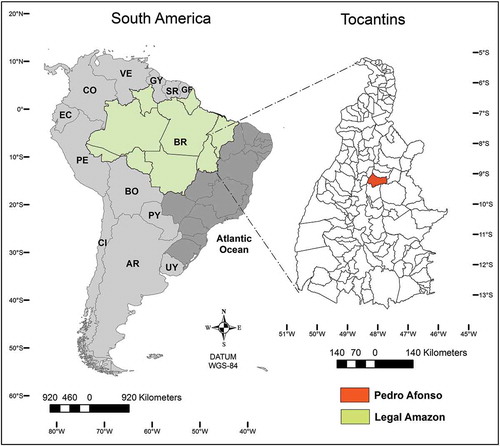
Our study area is in one of the newest regions of sugarcane expansion in Brazil. It is in the municipality of Pedro Afonso, in the state of Tocantins, located within Brazil’s ‘Legal Amazon’, a bio-administrative unit comprised of nine states (SUDAM, 2015). Traditionally, the state was known for its wide expanses of land used for cattle ranching and the predominance of landcovers typical of the cerrado (savanna) biome. By the early twenty-first century, it had become an important grain producer (Lapola et al., 2013). However, the introduction in 2008 of the first major sugarcane mill in the region, located in the municipality of Pedro Afonso (BUNGE, 2012), has greatly expanded the production of sugarcane, contributing to a great deal of LUCC in recent years. In a recent CONAB (Brazilian Government National Supply Company) survey, sugarcane crop area increased 60.2% from 2012 to 2013 in the state of Tocantins (CONAB, 2013a).

We chose the municipality of Pedro Afonso, in the center of the state (Figure 1) as an ideal place to test our mapping and LUCC analysis methods. The municipality has an area of 2051 km². Elevation averages about 200 m above sea level, and the climate is classified as tropical, according to Köppen-Geiger classification (Aw), with marked rainy and dry seasons. Vegetation is predominantly xerophytic, common in the cerrado (savanna biome). Forested areas have tree species occasionally 8–12 m high, while natural pasture areas contain sparse bushes 2–3 m high. The local economy is based on agriculture and cattle ranching. While Pedro Afonso municipality is among the top six second-harvest corn producers in the state, based on the average MODIS EVI profiles of cropland from this study, it appears that single crop soy or corn is the predominant form of agriculture (Montechese, 2013). The rivers that cut through the area allow the existence of some irrigated fields.

Figure 1. Study area.

The municipality stands out as both one of the largest soybean producers in the state and one that has received major investment for sugarcane cultivation for bioethanol production, especially from the Bunge mill company. Mill activities began with the first planting of sugarcane in July 2007, with a nursery of seedlings covering an area of 237 hectares. The construction of the Pedro Afonso mill, on the very site of the first plantation, began in January 2008. In July 2010, the mill began operation, albeit in an experimental mode, and it only became fully operational in May 2011, reaching more than 24,000 hectares planted in 2012 (BUNGE, 2012). Such circumstances allow for an understanding of the LUCC associated with the mill, since during our study period there were no other sugar mills within a radius of more than a thousand kilometers (PORTOSMA, 2011). We can assume, therefore, that all of the associated LUCC can be attributed to the presence and actions of this one mill. Finally, we know that sugarcane development in this region is a sensitive issue, given concerns about indirect LUCC in the adjacent Amazon biome (Arima, Richards, Walker, & Caldas, 2011; Walker, 2011). This study will provide insight as to whether at least in this case, sugarcane has the potential to push cattle ranching and other activities into other areas, especially should this region develop into a major sugarcane production hub, as some suspect (Nascimento & De Abreu, 2012).

3. Data and methods

To focus our research effort, we concentrate on mapping three LULC categories in the municipality: Sugarcane, Other Crops and Other Classes (Table 1). The agricultural calendar in the region begins in one calendar year with planting, and it ends in the following year with harvest. By convention, we refer to crop years (CY), followed by the calendar year during which crops were harvested. Our study maps LUCC from CY2008-CY2013.

Table 1. Land cover class description.

Class	Description
Sugarcane	Agricultural areas with sugarcane crop.
Other Crops	Agricultural areas where soybean predominates, but which also presents rice, beans or corn.
Other Classes	Natural vegetation typical of the Brazilian cerrado (savanna-like ecosystem), pasture, forest, built, and water bodies.

We first created an annual ground reference dataset of the three categories through visual interpretation and manual, on-screen delimitation of high-resolution satellite imagery, similar to what other researchers have done to map sugarcane areas in the state of São Paulo and throughout many states in Brazil as part of the Canasat Project (Aguiar et al., 2011; Mello et al., 2012; Rudorff et al., 2010). We then extracted the temporal profiles of MODIS 250-m Enhanced Vegetation Index (EVI) data for each class to determine specific time periods during the growing season where it is possible to separate the three LULC categories of the study. Using this information, we created the annual LUCC maps. We investigate the accuracy of the maps by comparing classified area with that provided by government agricultural statistics, and we calculate accuracies by comparing our maps with ground reference. Finally, we conduct intensity analysis.

3.1. Satellite remote sensing datasets

We downloaded freely available images from the Landsat 5 Thematic Mapper (TM) and Landsat 8 Operational Land Imager (OLI) sensors, both with a 30 m pixel size, as well as from the IRS-P6 sensor from RESOURCESAT-1 which has a 23.6 m pixel size. The following images were acquired during the crop phenological cycle (January to June): Landsat 5 TM (path/row 222/66) from February 1, 19 May 2008, 3 January 2008, 22 May 2009, 17 January 2009, 9 May 2010, 2010, and 12 May 2011; IRS-P6 image (path/row 327/83) from 30 June 2012; Landsat 8 OLI image (path/row 222/66) from 17 May 2013. In addition, 250-m, 16-day composite MOD13Q1 MODIS EVI data from 28 July 2007 to 1 November 2013 (145 images) were downloaded from the MODIS products database, a repository maintained by Embrapa Agroinformatics (https://www.modis.cnptia.embrapa.br), which provides images derived from the MOD13Q1 product prepared by the Land Processes Distributed Active Archive Center (LP DAAC; https://lpdaac.usgs.gov/) (Esquerdo, Antunes, & Andrade, 2011). This database provides Normalized Difference Vegetation Index (NDVI) and EVI images for all time periods from the Terra satellite. Data can be downloaded by state, already mosaicked, projected and in GeoTIFF format.

We worked exclusively with the Enhanced Vegetation Index (EVI) data. Vegetation indices like EVI typically provide values from 0 to 1, with higher values indicating higher levels of photosynthetically active biomass at the surface, and lower values indicating lower levels (Huete et al., 2002; Huete, Liu, Batchily, & Van Leeuwen, 1997). Thus, it is possible to distinguish certain crop types and vegetation types from how their phenological characteristics vary during a given year, and numerous researchers have used indices like EVI for this very purpose (Arvor et al., 2012; Galford et al., 2008; Rudorff et al., 2009; Zhang et al., 2008).

3.2. Ground reference dataset

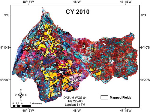
The identification and mapping of the Sugarcane and Other Crops categories (Table 1) were carried out from CY2008 to CY2013, using photo-interpretation techniques and also by using a false color composition based on the following combination that allowed us to distinguish annual crops from sugarcane and other classes: R: NIR; G: SWIR; B: RED (Landsat 5: 453; IRS-P6: 342; Landsat 8: 564). The short-wave infrared band (SWIR) is sensitive to variations in water content, in leafy vegetation as well as in soil. In the combination above, active vegetation appears in shades of red. When vegetation has a relatively lower moisture content, the reflection from the SWIR band will be relatively higher, meaning there is more contribution of green to the false color image, thus resulting in a more orange color. Even when sugarcane and soybeans are at their peak state at the same time, soybeans appear more orange and sugarcane more red. Agricultural field geometries are also quite different, allowing us to use this visual aspect to distinguish the two classes: sugarcane is much more rectangular with straighter field boundaries than annual crop fields. Bare soils and urban areas appear in blue towards gray colors. Using ArcGIS 10.1 ESRI software, thematic maps were created (Figure 2). The number of fields mapped for each crop year and category is shown in Table 2. We emphasize that this visual interpretation-based approach to create a ground reference dataset lacks the rigor associated with one developed from a properly designed field observation campaign. Given limited resources to conduct fieldwork, and the fact that data from the Canasat Project, mapping sugarcane across Brazil’s main growing regions, are not publically available, it was necessary for us to follow their established and well published visual interpretation methods to create a ground reference dataset on our own (Aguiar et al., 2011; Mello et al., 2012; Rudorff et al., 2010).

Table 2. Number of fields mapped by photo-interpretation techniques for reference data.

	Number of reference fields
Category/Crop year	CY2008	CY2009	CY2010	CY2011	CY2012	CY2013
Sugarcane	1	6	42	65	80	99
Other Crops	149	144	118	100	91	81
Total	150	150	160	165	171	180

Figure 2. Example of reference map created from Landsat and IRS-P6 images from the CY2010 in the study area.

3.3. MODIS masks

Based on the high-resolution ground reference dataset for each year, we extracted from the MODIS dataset from one to three ‘best interior pixels’ for each polygon, similar to that performed by Wardlow, Egbert, and Kastens (2007). These are pixels whose temporal profiles of the Enhanced Vegetation Index are relatively noise-free and not subject to edge effects. We then took the EVI time series of every polygon by category and adopted a ‘temporal composition’ (hereafter, TC) approach (Coutinho et al., 2013; de Souza, Mercante, Johann, Lamparelli, & Uribe-Opazo, 2015) to separate the Sugarcane from the Other Crops time series. We first calculated the mean EVI value at each time period for both categories for each year separately. This is plotted in Figure 3(a) for an example year (CY2010) (the bars at each point mark one standard deviation above and below the mean). This approach ensures that we preserve the variability in EVI values that exists across the landscape during each year due to differences in planting/harvesting times and precipitation, all of which affect EVI values. We then took the annual mean EVI time series and calculated the mean of those for each time period across all the years, giving us a mean of means. These data allowed us to detect the greatest EVI difference between Sugarcane and Other Crops during crop cycle development, allowing selection of the temporal window and the EVI thresholds that best separated the Sugarcane from the Other Crops categories. This was done separately for each year of the study (Figure 3(b)). We selected the temporal windows by identifying 3 consecutive periods when the difference between the means for each category was greatest. To determine the EVI thresholds, we chose the lower value as one standard deviation below the lowest of the multi-annual means, and the higher value as one standard deviation above the highest of the multi-annual means. In sum, the temporal window for TC1 was between January 1 and February 18, and TC2 was between April 7 and May 25. EVI thresholds were between 0.72–0.9 for Other Crops and 0.53–0.70 for Sugarcane.

Figure 3. A general overview of the methodology used in the process of pixel identification for each category and crop year. Example of image selected (a); creation of temporal compositions (b); definition of thresholds (c) and pixel identification (c, d).

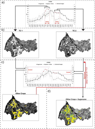
We then took TC1 shown in Figure 3(b) and selected from it only the pixels whose values fall within the chosen EVI threshold for Other Crops (Figure 3(c)). Then we excluded from TC2 the pixels from Other Crops and then applied a selection of pixels that fell within the Sugarcane threshold to obtain the sugarcane mask. Together, Other Crops and Sugarcane are presented in Figure 3(d). The pixels that satisfied neither threshold were classified as ‘Other classes’.

3.4. Map accuracy assessment

The information obtained from the reference and MODIS maps, for each crop and crop year, were compared to the official harvested area data from the Brazilian Institute for Geography and Statistics (IBGE) Municipal Agricultural Production census (IBGE, 2014). The official data for the Other Crops class were obtained by summing the cultivated crop area in the municipality (e.g. soybean, rice, beans and corn), with the exception of sugarcane. To compare the estimates, we calculated the mean error (ME), root mean square error (RMSE) and Willmott concordance index (d_r) (Willmott, Robeson, & Matsuura, 2012) (Eq. 1). The d_r coefficient defines the precision of the method and indicates the deviation between the estimated and observed values. This index varies between −1 and 1, where positive values closer to 1 have better concordance

(1)

where n = number of observations, O = observed area, E = estimated area and = mean observed area.

Reference maps were used to assess the accuracy of the maps produced with the MODIS data. For this purpose, pixel resample aggregation of the reference maps (30 m) was carried out to match the same resolution as the MODIS masks (250 m), thus allowing comparison. This allowed all the maps to be at the same spatial extent with 32,522 pixels each of 250 m × 250 m, wherein each pixel represents one of the three categories: Sugarcane, Other Crops or Other Classes. After that, we created a confusion matrix for each crop year and calculated quantity disagreement and allocation disagreement (Pontius & Millones, 2011). Quantity disagreement is an error where commission is positive and omission is zero, or when commission is zero and omission is positive. On the other hand, allocation disagreement would exist only if there were simultaneous positive commission and positive omission errors. Finally, the total disagreement is the sum of quantity disagreement and allocation disagreement (Aldwaik & Pontius, 2013; Pontius & Millones, 2011).

3.5. LUCC analysis

We took the MODIS-based maps and constructed traditional confusion matrices for each crop year. In addition, we analyzed the changes using intensity analysis, examining land change at three levels of analysis, starting from general to more detailed levels: time interval, category and transition. At each level, intensity analysis compares the observed changes to hypothetical uniform change, which is marked by a line indicated in accompanying figures (Aldwaik & Pontius, 2013; Zhou et al., 2014). Intensity analysis was performed using the package developed in Microsft Excel 2007 software available at https://sites.google.com/site/intensityanalysis/.

4. Results and discussion

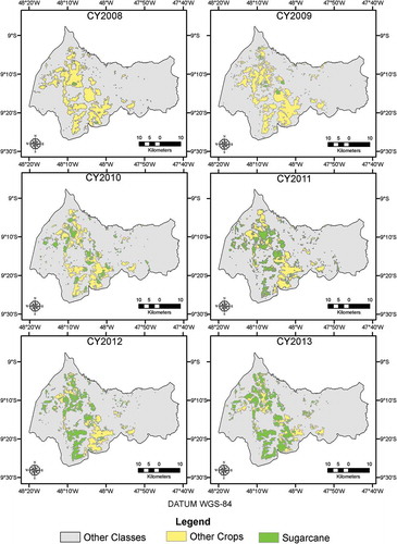
The spatial distribution of Sugarcane and Other Crops is shown in Figure 4. Visually, it appears that sugarcane expanded into other crop areas from CY2010, a dynamic likely driven by the opening of the Bunge Pedro Afonso sugarcane mill in 2008. In support of this interpretation, a recent survey with farmers carried out by the Brazilian Supply Company (CONAB, 2013b), regarding areas replaced by sugarcane crops in the state of Tocantins, revealed that 80% of new land for sugarcane in 2011/2012 was previously occupied by soybeans, whereas 20% was land previously used as pasture, in major constrast to other regions of Brazil.

Figure 4. Crop masks from CY2008 to CY2013 from MODIS data in the study area.

4.1. Accuracy assessment

The land area data obtained by the MODIS-based maps, reference maps, and IBGE are shown in Figure 5. The rise in Sugarcane area, with the inverse change in Other Crops areas is clearly observed across all sources, confirming the general visual pattern.

Figure 5. Land area data (ha) obtained from reference maps, MODIS masks and official data (IBGE).

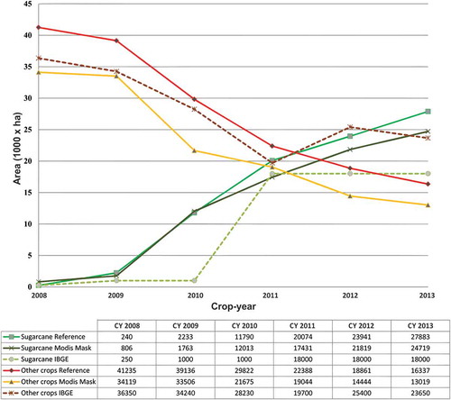
The MODIS-based data is most similar to the reference maps (Figure 5). The data from IBGE follows similar trends, with some important exceptions. In CY2011 and CY2012, IBGE data for Other Crops diverge from the other sources, and IBGE sugarcane data show the exact same value for two years in a row, while the other sources show an increase. This observation is consistent with others who have demonstrated significant differences between official IBGE statistics and mapping data from remote sensing.

Table 3 provides statistical comparisons among the data from the MODIS masks, reference maps and IBGE. Analyzing both the RMSE and ME in the Sugarcane category, the data from the MODIS masks are closely related to the reference maps, as affirmed by a 0.92 concordance index. In comparison to the IBGE official data, the gap is larger due to the IBGE not following the land area increase between the crop years. For the Other Crops class, the MODIS mask and reference maps comparison achieved a concordance index of 0.69, and underestimated 5328 ha on average. The reference maps versus IBGE comparison reached a 0.87 concordance index and, using the ME, the crop area for Other Crops was overestimated by 3482 ha on average. However, as observed in Figure 5, it did not follow the same trend from CY2011 onwards.

Table 3. Statistical analysis from land area data.

	Sugarcane			Other Crops
Comparison	ME (ha)	RSME (ha)	dr	ME (ha)	RSME (ha)	dr
Mask vs. RFM	−1268.68	1919.0	0.9203	−5328.78	5633.5	0.6961
Mask vs. IBGE	3716.6	5510.8	0.7736	−5293.96	6855.4	0.4718
RFM vs. IBGE	4985.3	6522.1	0.7108	34.82	5063.5	0.8746

ME: mean error; RSME: root square mean error; d_r: Willmott’s index of agreement; RFM: reference maps; Mask: MODIS Mask; IBGE: official data.

We can also compare our results to those from Nascimento and De Abreu (2012), who estimated crop areas in Pedro Afonso for CY2010: 21,302 ha for soybeans, 6210 ha for sugarcane, 5332 ha for prepared soil (bare soil). If we assume that the bare soil is newly harvested areas or prepared for sugarcane cultivation, summing bare soil with sugarcane from this report yields a value very close to the 12,000 ha of sugarcane we mapped for that year. These authors also mentioned the importance of the process of sugarcane taking over soybeans, verifying that some farmers were leasing their land to the sugarcane mill.

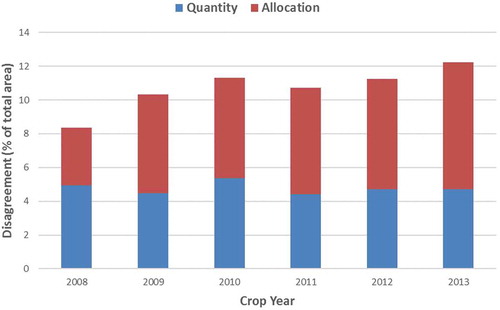
Finally, it is important to emphasize that there are two main sources of error in land cover area estimations using satellite images: the presence of mixed pixels and the misclassification of pure pixels. Thus, the accuracy of area estimates is linked with the accuracy of image classification (Gallego, 2004). The disagreement between the ground reference maps and the MODIS-based maps for each cropping year is summarized in Figure 6. The total disagreement is separated into two major components: quantity disagreement and allocation disagreement (Pontius & Millones, 2011). The overall agreement is 100% minus the total disagreement, 91.65, 89.68, 88.68, 89.27, 88.75 and 87.78% for each crop year, respectively, in accordance with Figure 6. The quantity disagreement was stable, meaning that the mapping approach obtained an error of 4.76% on average, in terms of proportion of categories. Regarding allocation disagreement, the CY2013 achieved the higher error (7.52%), in terms of spatial distribution of the categories.

Figure 6. Components of disagreement between the reference maps and MODIS masks.

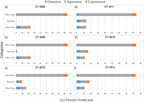
Figure 7 summarizes the agreement, omission disagreement, and commission disagreement for each category and map that we have created, where the vertical axis shows the categories while the horizontal axis shows the percentage of total area. Figure 7 shows that Other Classes is the largest category in the study area, and also that the Sugarcane category increases over the crop years. Moreover, it shows for the Other Classes category that the commission disagreement (average 6.71%) is greater than the omission disagreement (average 2.76%) in all cropping years, and it was thus overestimated by the method. In contrast, Sugarcane and Other Crops were underestimated, with an omission disagreement greater than the commission disagreement. Indeed, omission for one category is commission for a different category. This shows that some pixels that belonged to the Sugarcane and/or Other Crops categories, according to the reference map, have not been respectively classified using the MODIS-based data, and were thus wrongly allocated to the Other Classes category. It is important to note that the spatial resolution of the MODIS sensor (250 m) often causes pixels at the edge and within small cropland areas to have a higher degree of spectral mixing with other elements that are present in the vicinity (de Souza et al., 2015; Lobell & Asner, 2004; Wardlow & Egbert, 2008), leading to omission errors for Other Crops and increasing commission errors for Other Classes.

Figure 7. Category-level analysis of agreement, omission disagreement and commission disagreement for the MODIS masks.

4.2. Change analysis

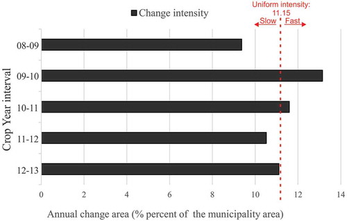
Figure 8 provides results of the interval level intensity analysis, where the vertical axis shows crop year intervals and each horizontal bar is the observed change intensity. The uniform line (in red) is the rate of change that would be present if the rate of change were uniform across the time periods. If an interval’s bar ends before the uniform line (red line), then the interval’s annual change is considered slow; if the bar is above the line, then the interval’s annual change is considered fast (Aldwaik & Pontius, 2013). Figure 8 shows the annual change was fast during the CY09-CY10 and CY10-CY11 intervals, which may be related to the expansion of sugarcane fields from the nursery of seedlings to other mill areas, after the deployment of the sugarcane mill in the region in 2008 (BUNGE, 2012). Change was slower in the subsequent intervals CY11–12 and 12–13, perhaps as the rate of leasing properties for sugarcane decelerated in relation to the earlier years.

Figure 8. Intensity of annual change in area within each cropping year interval.

The time interval analysis gives a general picture of land change, but it does not reveal anything about what categories contributed to that change, which is why we move next to the category level intensity analysis as show in Figure 9. Each category has a pair of horizontal bars, where the bars to the right show the size of the annual gain intensity and annual loss intensity of each category in terms of the relative sizes of the categories, while the bars that extend to the left are the annual gain in area and annual loss in area. The red line shows what the level of intensity would be if change in the category were distributed uniformly across the study area. If an interval’s bar ends before the uniform line (red line), then we assume the category is dormant; if an interval’s bar extends beyond the uniform line, then we affirm the category is active (Aldwaik & Pontius, 2013).

Figure 9. Category intensity analysis for crop year intervals. Bars that extend to the left show gross annual area gains and losses in the study area, while bars that extend to the right show intensity of annual gains and losses within each category.

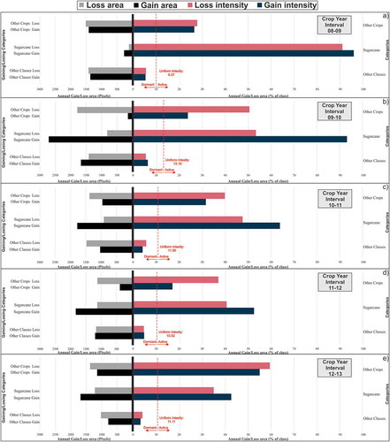
Gains and losses in Other Classes were dormant, while the gains and losses of Sugarcane and Other Crops were active for all cropping season intervals. This indicates that Sugarcane and Other Crops experienced gains and losses more intensively than the landscape in general (Other Classes). Proportionally, in the CY2008–2009 interval (Figure 9(a)), Sugarcane gained and lost more intensively than Other Crops and Classes. Recall that Sugarcane’s category was extremely small in the first year – it was a plantation of seedlings – and the mill was constructed on that very place, displacing the sugarcane elsewhere, resulting in a very large percentage change. From the next interval (2009–2010) onward, Sugarcane and Other Crops have a land dynamic greater than uniform intensity (active categories). According to Zhou et al. (2014), such a trend is persistent, since the same dynamic is seen across the entire series of time intervals.

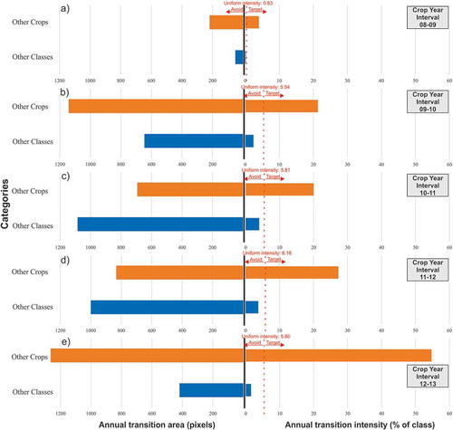
We now know that Sugarcane and Other Crops are the categories actively driving land change in the study area. The next level of analysis, the transition level, allows for determining whether gains or losses from one category to another are part of a systematic targeting, or whether they are simply occurring in proportion to the relative sizes of the categories in question. Statistics can be calculated for every possible transition, but we are mainly interested in the dynamics between Sugarcane and Other Crops, so we calculate the transition intensity for Sugarcane in relation to Other Crops and Other Classes to confirm whether Sugarcane is actively targeting the Other Crops category. Figure 10 presents the annual transition area on the left side and the annual transition intensity on right side, where the vertical axis shows the categories that lost area to Sugarcane. When we analyze the left side in terms of the size of the annual transition, the Other Crops category appears to contribute the most to Sugarcane gains. However, the transition from Other Classes to Sugarcane had a substantial number of pixels, especially in the CY10–11 and CY11–12 intervals (Figure 10(c,d)). Nevertheless, the right side values clearly verify Sugarcane gaining much more intensively from Other Crops than Other Classes, which map error alone can not explain. Furthermore, in all the crop year intervals, the intensity values for Other Crops exceed uniform intensity (red line). These results support the hypothesis that Sugarcane is replacing Other Crops in a targeted, systematic way in all time intervals. If Sugarcane had gained area uniformly across the landscape, we would expect to see much lower intensity levels for Other Crops and Other Classes nearer the uniform intensity line.

Figure 10. Transition intensity analysis to Sugarcane category for the crop year intervals. Bars that extend to the left show gross annual area of transitions to Sugarcane, while bars that extend to the right show intensity of annual transitions to Sugarcane within the Other Crops and Other Classes categories.

It is difficult to confirm what policy or socio-economic dynamics are a part of explaining the land change dynamics above without interviews in the field with government officials, industry representatives, and farmland owners. Such work was beyond the scope of the current project, but we can look to the Sugarcane Zoning for the state, and a brief review of news reports from the region, to shed some light on the socio-environmental dynamics of land change, spurring new questions for research. According to the Sugarcane Zoning, the state of Tocantins has suitable areas for sugarcane expansion classified as ‘Medium’ suitability, taking into account environmental, economic and social aspects. In summary, the zoning delimits approximately 1 million ha with pasture and 73 thousand ha with agriculture suitable for sugarcane cultivation in the state (Manzatto et al., 2009). The Sugarcane Zoning gives priority to land currently underutilized or occupied by livestock or degraded pastures. However, the zoning takes no account of other factors such as logistics and infrastructure, the cost of land to be bought or leased, and other market factors important in projecting land use in specific regions (Almeida, 2012). Unfortunately, the Sugarcane Zoning was not done at a scale detailed enough to evaluate at the level of the Pedro Afonso municipality to determine the extent to which land managers are adhearing to zoning guidelines in converting land to sugarcane production. Concerning the social relations driving land change, we know that the large international group Bunge, which constructed and runs the mill, is able to secure raw material by both leasing and buying land from annual crop producers (especially soybean producers) to plant sugarcane (COPERCANA, 2012). This dynamic then begs two main questions: is the acquisition of the land done in a socially just way, and if farmers who sell or lease still want to produce soybeans, where do they go and what are the subsequent indirect LUCC consequences? Some producers lament the changes, expressing fear about a future when more and more leave day to day life on the farm (FOLHA, 2012), a finding as well from Petrini, Rocha, and Brown (2017). Others complain that the leasing deals being made are undervaluing farmland in the region, citing much higher average amounts paid on leases in other parts of the country (T1, 2015). Systematically assessing indirect LUCC is beyond the focus of our study, but our results suggest that the dynamic is possible within and adjacent to Pedro Afonso. Soybean cultivated area increased dramatically in neighboring municipalities during our study period, suggesche mill in Pedro Afonso may have acquired access to farmland outside the study area in order to continue planting soybeans.¹

It is important to recognize the main limitations of the remote sensing approach employed in the study. We relied on high-resolution satellite data to manually digitize, on-screen, all of the polygons of Sugarcane and Other Crop production in the study area, similar to what is already done in the Canasat Project, to produce the ground reference dataset for mapping these classes with MODIS. This is a laborious, costly, and time-consuming process. (Future work could potentially explore the use of object-based image analysis.) If we were to extend our visual-interpretation work to larger regions, even more time would be taken, and then the question is why not just use the high-resolution maps for assessing LUCC and abandon efforts to map using MODIS? Things brings up the additional issue that the MODIS and Landsat data cannot be considered truly independent observations since they are collected under similar conditions; thus using one to detect differences in the other produces biased results. This research has shown promise, however, in using MODIS EVI profiles to detect differences between sugarcane and crop cultivation, and future work could confirm this with determining MODIS-based map accuracy against independently collected ground reference data. Next, the task would be to test how applicable the temporal windows and EVI thresholds determined for this study area are in adjacent areas, which would be a step in a study of indirect LUCC caused by the opening of the mill. Significant results could then be extended spatially from there until we reach a substantially different planting and climate regime. Further field campaigns to collect ground reference data, supplemented with existing cultivation calendars would then help to determine the needed windows and thresholds for the temporal composition procedure.

5. Conclusions

In this paper, we addressed the need for both accurate maps of LUCC and sound statistical methods for assessing land change in areas experiencing expansion of biofuel crop production. Our approach involved mapping Sugarcane, Other Crops, and Other Classes using MODIS EVI data in a municipality undergoing rapid expansion of sugarcane production. Using intensity analysis we were able to produce three main findings: 1) we confirmed that change in the landscape is occurring at a pace that exceeds uniform change in 2 of the 5 time periods studied (corresponding to deployment of the sugarcane mill in the region); 2) Sugarcane and Other Crops are the categories contributing most to that change; and 3) that Sugarcane is systematically targeting Other Crops for conversion. Our review of previous work on the question of the LUCC dynamics of sugarcane expansion in Brazil showed tremendous variability in the way that land change results were presented, complicating efforts to compare results. The very methodical approach of intensity analysis permits users to take a simple change matrix derived from comparing land use/land cover maps from two different periods and make all the calculations needed for careful and systematic evaluations of land change. When dealing with the sensitive topics of the socio-environmental dynamics of food vs. fuel production, it is especially important that policy makers, civil society organizations, industry and other interested parties rely on information produced from such a standard and transparent form of analysis.

Acknowledgements

This work was supported in part by grants to the authors from the Coordination for the Improvement of Higher Level Personnel (CAPES). The third author recognizes fellowship support from Fulbright and the São Paulo Research Foundation (FAPESP, 2015/194375), in addition to grant support from NSF-BCS-GSS 1227160.

Disclosure statement

No potential conflict of interest was reported by the authors.

Additional information

Funding

This work was supported by the Coordenação de Aperfeiçoamento de Pessoal de Nível Superior;Fundação de Amparo à Pesquisa do Estado de São Paulo [2015/194375];Fulbright.

Notes

1. According to the IBGE (2014), the adjacent municipalities of Bom Jesus do Tocantins and Tupirama as a whole increased soybean area by 6000 ha and sugarcane area by 4080 ha, from CY2011 to CY2013.

References

- Adami, M., Rudorff, B.F.T., Freitas, R.M., Aguiar, D.A., Sugawara, L.M., & Mello, M.P. (2012). Remote sensing time series to evaluate direct land use change of recent expanded sugarcane crop in Brazil. Sustainability, 4(12), 574–585. doi:10.3390/su4040574
- Aguiar, D.A., Rudorff, B.F.T., Silva, W.F., Adami, M., & Mello, M.P. (2011). Remote sensing images in support of environmental protocol: Monitoring the sugarcane harvest in São Paulo State, Brazil. Remote Sensing, 3(12), 2682–2703. doi:10.3390/rs3122682
- Aldwaik, S.Z., & Pontius, R.G., Jr. (2013). Map errors that could account for deviations from a uniform intensity of land change. International Journal of Geographical Information Science, 27(9), 1717–1739. doi:10.1080/13658816.2013.787618
- Aldwaik, S.Z., & Pontius, R.G. (2012). Intensity analysis to unify measurements of size and stationarity of land changes by interval, category, and transition. Landscape and Urban Planning, 106(1), 103–114. doi:10.1016/j.landurbplan.2012.02.010
- Almeida, M. (2012). Analysing the Brazilian sugarcane agroecological zoning: Is this government policy capable of avoiding adverse effects from land-use change? Victoria University of Wellington. Retrieved from http://hdl.handle.net/10063/2418
- Arima, E.Y., Richards, P., Walker, R., & Caldas, M.M. (2011). Statistical confirmation of indirect land use change in the Brazilian Amazon. Environmental Research Letters, 6(2), 24010. doi:10.1088/1748-9326/6/2/024010
- Arvor, D., Meirelles, M., Dubreuil, V., Bégué, A., & Shimabukuro, Y.E. (2012). Analyzing the agricultural transition in Mato Grosso, Brazil, using satellite-derived indices. Applied Geography, 32(2), 702–713. doi:10.1016/j.apgeog.2011.08.007
- Bégué, A., Lebourgeois, V., Bappel, E., Todoroff, P., Pellegrino, A., Baillarin, F., & Siegmund, B. (2010). Spatio-temporal variability of sugarcane fields and recommendations for yield forecast using NDVI. International Journal of Remote Sensing, 31(20), 5391–5407. doi:10.1080/01431160903349057
- Braimoh, A.K. (2006). Random and systematic land-cover transitions in northern Ghana. Agriculture, Ecosystems & Environment, 113(1–4), 254–263. doi:10.1016/j.agee.2005.10.019
- Brown, J., Jepson, W., Kastens, J., Wardlow, B., Lomas, J., & Price, K. (2007). Multitemporal, moderate-spatial-resolution remote sensing of modern agricultural production and land modification in the Brazilian Amazon. GIScience & Remote Sensing, 44(2), 117–148. doi:10.2747/1548-1603.44.2.117
- Brown, J.C., Hanley, E., Bergtold, J., Caldas, M., Barve, V., Peterson, D., … Earnhart, D. (2014). Ethanol plant location and intensification vs. extensification of corn cropping in Kansas. Applied Geography, 53, 141–148. doi:10.1016/j.apgeog.2014.05.021
- BUNGE. (2012). Sustainability report. Retrieved December 1, 2015, from http://www.bunge.com.br/sustentabilidade/2012/eng/ra/09.htm
- Carrão, H., Gonçalves, P., & Caetano, M. (2008). Contribution of multispectral and multitemporal information from MODIS images to land cover classification. Remote Sensing of Environment, 112(3), 986–997. doi:10.1016/j.rse.2007.07.002
- Castro, S.S., Abdala, K., Aparecida Silva, A., & Borges, V. (2010). A expansão da cana-de-açúcar no cerrado e no estado de goiás: Elementos para uma análise espacial do processo. Boletim Goiano de Geografia, 30(1), 171–191. doi:10.5216/bgg.v30i1.11203
- CONAB. (2013a). Acompanhamento de safra brasileira: cana-de-açúcar, terceiro levantamento, abril/2013. Brasília. Retrieved from http://www.conab.gov.br/OlalaCMS/uploads/arquivos/13_04_09_10_30_34_boletim_cana_portugues_abril_2013_4o_lev.pdf
- CONAB. (2013b). Perfil do Setor do Açúcar e do Álcool no Brasil. Retrieved from http://www.conab.gov.br/OlalaCMS/uploads/arquivos/13_10_02_11_28_41_perfil_sucro_2012.pdf
- COPERCANA. (2012). Cana “atropela” soja em pólo do Tocantins. Retrieved November 1, 2015, from http://www.copercana.com.br/index.php?xvar=ver-ultimas&id=2603
- Coutinho, A.C., Esquerdo, J.C.D.M., Oliveira, L.S., & Lanza, D.A. (2013). Methodology for systematical mapping of annual crops in Mato Grosso do Sul state (Brazil). Geografia, 38, 45–54. Retrieved from https://www.geopantanal.cnptia.embrapa.br/publicacoes/4geo/p3_45-54.pdf
- de Souza, C.H.W., Mercante, E., Johann, J.A., Lamparelli, R.A.C., & Uribe-Opazo, M.A. (2015). Mapping and discrimination of soya bean and corn crops using spectro-temporal profiles of vegetation indices. International Journal of Remote Sensing, 36(7), 1809–1824. doi:10.1080/01431161.2015.1026956
- Esquerdo, J.C.D.M., Antunes, J.F.G., & Andrade, J.C. (2011). Desenvolvimento do Banco de Produtos MODIS na Base Estadual Brasileira. In XV Simposio Brasileiro de Sensoriamento Remoto, 30 April–05 May 2011, Curitiba, Brazil, edited by INPE
- FOLHA. (2012). Cana chega ao Tocantins com irrigação. Retrieved May 20, 2011, from http://www1.folha.uol.com.br/fsp/mercado/85393-cana-chega-ao-tocantins-com-irrigacao.shtml
- Galford, G.L.G., Mustard, J.J.F., Melillo, J., Gendrin, A., Cerri, C.C.E.P., & Cerri, C.C.E.P. (2008). Wavelet analysis of MODIS time series to detect expansion and intensification of row-crop agriculture in Brazil. Remote Sensing of Environment, 112(2), 576–587. doi:10.1016/j.rse.2007.05.017
- Gallego, F.J. (2004). Remote sensing and land cover area estimation. International Journal of Remote Sensing, 25(15), 3019–3047. doi:10.1080/01431160310001619607
- Huang, J., Pontius, R.G., Li, Q., & Zhang, Y. (2012). Use of intensity analysis to link patterns with processes of land change from 1986 to 2007 in a coastal watershed of southeast China. Applied Geography, 34(3), 371–384. doi:10.1016/j.apgeog.2012.01.001
- Huete, A., Didan, K., Miura, T., Rodriguez, E., Gao, X., & Ferreira, L. (2002). Overview of the radiometric and biophysical performance of the MODIS vegetation indices. Remote Sensing of Environment, 83(1–2), 195–213. doi:10.1016/S0034-4257(02)00096-2
- Huete, A.R., Liu, H.Q., Batchily, K., & Van Leeuwen, W. (1997). A comparison of vegetation indices over a global set of TM images for EOS-MODIS. Remote Sensing of Environment, 59(3), 440–451. doi:10.1016/S0034-4257(96)00112-5
- IBGE. (2014). Sistema IBGE de Recuperação Automática - SIDRA. Retrieved January 1, 2015, from http://www.sidra.ibge.gov.br
- Lapola, D.M., Martinelli, L.A., Peres, C.A., Ometto, J.P.H.B., Ferreira, M.E., Nobre, C.A., … Vieira, I.C.G. (2013). Pervasive transition of the Brazilian land-use system. Nature Climate Change, 4(1), 27–35. doi:10.1038/nclimate2056
- Lebourgeois, V., Begue, A., Degenne, P., Bappel, E., Lebourgeois, B.V., Begue, A., … Bappel, E. (2010). Improving harvest and planting monitoring for smallholders with geospatial technology: The Reunion Island experience. International Sugar Journal, 109, 109–119. Retrieved from http://hal.cirad.fr/cirad-00664053
- Lobell, D.B., & Asner, G.P. (2004). Cropland distributions from temporal unmixing of MODIS data. Remote Sensing of Environment, 93(3), 412–422. doi:10.1016/j.rse.2004.08.002
- Lunetta, R.S., Shao, Y., Ediriwickrema, J., & Lyon, J.G. (2010). Monitoring agricultural cropping patterns across the Laurentian Great Lakes Basin using MODIS-NDVI data. International Journal of Applied Earth Observation and Geoinformation, 12(2), 81–88. doi:10.1016/j.jag.2009.11.005
- Manning, P., Taylor, G., & Hanley, M.E. (2014). Bioenergy, food production and biodiversity - An unlikely alliance? GCB Bioenergy, n/a-n/a. doi:10.1111/gcbb.12173
- Manzatto, C.V., Assad, E.D., Bacca, J.F.M., Zaroni, M.J., & Pereira, S.E.M. (2009). Zoneamento Agroecológico da Cana-de Açúcar: Expandir a produção, preservar a vida, garantir o futuro. Rio de Janeiro: Embrapa Solos.
- Martinelli, L.A., & Filoso, S. (2008). Expansion of sugarcane ethanol production in Brazil: Environmental and social challenges. Ecological Applications : A Publication of the Ecological Society of America, 18(4), 885–898. doi:10.1890/07-1813.1
- Mello, M., Adami, M., Rudorff, B., & Aguiar, D. (2012, July 10–13). Canasat project accuracy assessment of sugarcane thematic maps. In Proceeding of the 10th International Symposium on Spatial Accuracy Assessment in Natural Resources and Environmental Sciences (pp. 281–286). Florianopolis-SC, Brazil. Retrieved from http://www.dsr.inpe.br/~mello/publications/files/Mello2012a_Canasat_Project_accuracy_assessment.pdf
- Montechese, M.A. (2013, November 26–28). Produção de Milho Safrinha nos Estados de Maranhão, Piauí, e Tocantins. Milho Safrinha, XII Seminário Nacional. Dourados, MS. Retrieved from http://www.cpao.embrapa.br/cds/milhosafrinha2013/palestras/11MARCIO-A.MONTECHESE.pdf
- Nascimento, H.R., & De Abreu, Y.V. (2012). Geotecnologias e o Planejamento da Agricultura de Energia. Málaga, Espanha: Eumed.Net, Universidad de Málaga. Retrieved from http://www.eumed.net/libros/ciencia/2012/4/index.htm
- Nassar, A.M., Rudorff, B.F.T., Antoniazzi, L.B., Aguiar, D.A., De Bacchi, M.R.P., & Adami, M. (2008). Chapter 3 Prospects of the sugarcane expansion in Brazil : Impacts on direct and indirect land use changes. In Sugarcane ethanol: Contributions to climate change mitigation and the environment (pp. 63–93). Wageningen: Wageningen Academic Publishers.
- Petrini, M.A., Rocha, J.V., & Brown, J.C. (2017). Mismatches between mill-cultivated sugarcane and smallholding farming in Brazil: Environmental and socioeconomic impacts. Journal of Rural Studies, 50, 218–227. doi:10.1016/j.jrurstud.2017.01.009
- Pontius, R.G., & Millones, M. (2011). Death to Kappa: Birth of quantity disagreement and allocation disagreement for accuracy assessment. International Journal of Remote Sensing, 32(15), 4407–4429. doi:10.1080/01431161.2011.552923
- PORTOSMA. (2011). Etanol do Tocantins vai ser escoado pelo Itaqui. Retrieved January 1, 2016, from http://www.portosma.com.br/noticias/noticia.php?id=2573
- Rathmann, R., Szklo, A., & Schaeffer, R. (2010). Land use competition for production of food and liquid biofuels: An analysis of the arguments in the current debate. Renewable Energy, 35(1), 14–22. doi:10.1016/j.renene.2009.02.025
- Romero-Ruiz, M.H., Flantua, S.G.A., Tansey, K., & Berrio, J.C. (2012). Landscape transformations in savannas of northern South America: Land use/cover changes since 1987 in the Llanos Orientales of Colombia. Applied Geography, 32(2), 766–776. doi:10.1016/j.apgeog.2011.08.010
- Rudorff, B.F.T., Adami, M., De Aguiar, D.A., Gusso, A., Da Silva, W.F., & De Freitas, R.M. (2009). Temporal series of EVI/MODIS to identify land converted to sugarcane. In 2009 IEEE International Geoscience and Remote Sensing Symposium (pp. IV-252–IV-255). IEEE. doi:10.1109/IGARSS.2009.5417326
- Rudorff, B.F.T., de Aguiar, D.A., da Silva, W.F., Sugawara, L.M., Adami, M., & Moreira, M.A. (2010). Studies on the rapid expansion of sugarcane for ethanol production in São Paulo State (Brazil) using landsat data. Remote Sensing, 2(4), 1057–1076. doi:10.3390/rs2041057
- Sakamoto, T., Wardlow, B.D., Gitelson, A.A., Verma, S.B., Suyker, A.E., & Arkebauer, T.J. (2010). A two-step filtering approach for detecting maize and soybean phenology with time-series MODIS data. Remote Sensing of Environment, 114(10), 2146–2159. doi:10.1016/j.rse.2010.04.019
- Sant’Anna, A.C., Shanoyan, A., Bergtold, J.S., Caldas, M.M., & Granco, G. (2016). Ethanol and sugarcane expansion in Brazil: What is fueling the ethanol industry? International Food and Agribusiness Management Review, 19(4), 163–182. doi:10.22434/IFAMR2015.0195
- Scarlat, N., & Dallemand, J.-F. (2011). Recent developments of biofuels/bioenergy sustainability certification: A global overview. Energy Policy, 39(3), 1630–1646. doi:10.1016/j.enpol.2010.12.039
- Schlesinger, S. (2014). Biocombustíveis : energia não mata a fome. Retrieved January 1, 2016, from http://fase.org.br/wp-content/uploads/2014/12/publicacao_impactos_biocombustiveis_mt.pdf
- Silva, A.A., & Miziara, F. (2011). Avanço do setor sucroalcooleiro e expansão da fronteira agrícola em Goiás. Pesquisa Agropecuária Tropical, 41(3), 399–407. doi:10.5216/pat.v41i3.11054
- SUDAM. (2015). Legislação da Amazônia. Retrieved August 1, 2015, from http://www.sudam.gov.br/index.php/institucional?id=86
- T1. (2015). Produtores reclamam que BUNGE desvaloriza terras em arrendamentos no Tocantins. Retrieved November 1, 2015, from http://m.t1noticias.com.br/agronegocio/produtores-reclamam-que-bunge-desvaloriza-terras-em-arrendamentos-no-tocantins/68979/
- UNICA. (2008). Relatório de sutentabilidade 2008. Retrieved January 1, 2016, from http://www.unica.com.br/download.php?idSecao=17&id=38415501
- UNICA. (2015). Sugarcane – One plant, Many Solutions. Retrieved November 1, 2015, from http://www.unica.com.br/download.php?idSecao=17&id=19111332
- Valentine, J., Clifton-Brown, J., Hastings, A., Robson, P., Allison, G., & Smith, P. (2012). Food vs. fuel: The use of land for lignocellulosic “next generation” energy crops that minimize competition with primary food production. GCB Bioenergy, 4(1), 1–19. doi:10.1111/j.1757-1707.2011.01111.x
- Vieira, M.A., Formaggio, A.R., Rennó, C.D., Atzberger, C., Aguiar, D.A., & Mello, M.P. (2012). Object based image analysis and data mining applied to a remotely sensed Landsat time-series to map sugarcane over large areas. Remote Sensing of Environment, 123, 553–562. doi:10.1016/j.rse.2012.04.011
- Walker, R. (2011). The impact of Brazilian biofuel production on Amazônia. Annals of the Association of American Geographers, 101(4), 929–938. doi:10.1080/00045608.2011.568885
- Wardlow, B., Egbert, S., & Kastens, J. (2007). Analysis of time-series MODIS 250 m vegetation index data for crop classification in the U.S. Central Great Plains. Remote Sensing of Environment, 108(3), 290–310. doi:10.1016/j.rse.2006.11.021
- Wardlow, B.D., & Egbert, S.L. (2008). Large-area crop mapping using time-series MODIS 250 m NDVI data: An assessment for the U.S. Central Great Plains. Remote Sensing of Environment, 112(3), 1096–1116. doi:10.1016/j.rse.2007.07.019
- Weng, Q. (2002). Land use change analysis in the Zhujiang Delta of China using satellite remote sensing, GIS and stochastic modelling. Journal of Environmental Management, 64(3), 273–284. doi:10.1006/jema.2001.0509
- Willmott, C.J., Robeson, S.M., & Matsuura, K. (2012). A refined index of model performance. International Journal of Climatology, 32(13), 2088–2094. doi:10.1002/joc.2419
- Zhang, X., Sun, R., Zhang, B., & Tong, Q. (2008). Land cover classification of the North China Plain using MODIS_EVI time series. ISPRS Journal of Photogrammetry and Remote Sensing, 63(4), 476–484. doi:10.1016/j.isprsjprs.2008.02.005
- Zhou, P., Huang, J., Pontius, R., & Hong, H. (2014). Land classification and change intensity analysis in a coastal watershed of Southeast China. Sensors, 14(7), 11640–11658. doi:10.3390/s140711640