Human drivers, biophysical changes, and climatic variation affecting contemporary cropping proportions in the northern prairie of the U.S

ABSTRACT

Grassland to cropland conversion in the northern prairie of the United States has been a topic of recent land use change studies. Within this region more corn and soybeans are grown now (2017) than in the past, but most studies to date have not examined multi-decadal trends and the synergistic web of socio-ecological driving forces involved, opting instead for short-term analyses and easily targeted agents of change. This paper examines the coalescing of biophysical and socioeconomic driving forces that have brought change to the agricultural landscape of this region between 1980 and 2013. While land conversion has occurred, most of the region’s cropland in 2013 had been previously cropped by the early 1980s. Furthermore, the agricultural conditions in which crops were grown during those three decades have changed considerably because of non-biophysical alterations to production practices and changing agricultural markets. Findings revealed that human drivers played more of a role in crop change than biophysical changes, that blending quantitative and qualitative methods to tell a more complete story of crop change in this region was difficult because of the synergistic characteristics of the drivers involved, and that more research is needed to understand how farmers make crop choice decisions.

KEYWORDS:

• U.S. northern prairie
• crop proportion change
• land use change
• web of drivers
• corn
• soybeans

1. Introduction

Cultivated crop production is one of the more indelible changes that humans have brought upon the Earth. This agricultural land use causes soil erosion (James, 2011; Trimble, 1974), alters hydrologic flows (Kim, Amalya, Chescheir, Skaggs, & Nettles, 2013), changes water quality and quantity (Power, 2010; Schwarz, Jacque, Dickens, Rogers, & Thompson, 1990), increases sedimentation rates (Hupp, Noe, Schenk, & Benthem, 2013), releases sequestered carbon (Liu, Tan, Li, Zhao, &Yuan, 2011; Tan et al., 2005), influences regional weather conditions (Chase, Pielke, Kittel, Baron, & Stohlgren, 1999; Marshall, Pielke, & Steyaert, 2003), and impairs wildlife habitat (Czech, Krausman, & Devers, 2000). Crop agriculture has also given birth to great civilizations, led to mass urbanization, and feeds the planet’s more than seven billion inhabitants.

Agricultural regions and their crops have evolved over space and time for various reasons and to various magnitudes, often because of underlying biophysical conditions, climate variability, and changing socioeconomic systems at multiple scales. For example, the Khabur Plains of northeastern Syria has cycled between small grains production and desertification over several millennia of human occupancy (Conniff, 2012). More recently, cropland in the Piedmont of the Southeastern United States (U.S.), once a leading cotton producing region, has been converted to pasture or hay land for cattle, returned to forest, or urbanized (Hart, 2001; Napton, Auch, Headley, & Taylor, 2010). The Midwestern Corn Belt of the U.S. has benefited from the synergy of favorable biophysical conditions that include a climate of ‘adequate moisture, and a warm growing season’ (Hudson, 1994, 15) that enabled widespread cropping across the region. California’s Mediterranean climate created nearly perfect growing conditions with respect to temperatures, but precipitation deficits warranted widespread irrigation throughout the Central Valley to produce its over 200 agricultural products (Hart, 2003a; Jelinek, 1979; Soulard & Wilson, 2015). Illinois Corn Belt and California Central Valley farmers first grew wheat before switching to more lucrative crops (Hudson, 1994; Jelinek, 1979; Prince, 1997). Substantial climatic variability, such as the drought of the 1930s, brought into question whether parts of the Great Plains should be cropland (Worster, 1979), but management improvements, technological changes, and perhaps shorter droughts have allowed crop production to remain one of the leading land uses in the region (Drummond et al., 2012). Continued climate change may alter current cropping capabilities in detrimental ways for some areas while enhancing or enabling farming in others (Lotze-Campen, 2011). A new transformation has begun on the northern prairie of the U.S. where producers who have typically grown small grains and hay have adopted agricultural practices more akin to those in the Corn Belt. We explore potential reasons why this change is occurring.

Land use change researchers tend to investigate driving forces that facilitate change. Often they look at a combination of both human and biophysical drivers to better understand the synergistic processes involved (e.g. Levers, Butsic, Verburg, Müller, & Kuemmerle, 2016; Serra, Pons, & Sauri, 2008; Smaliychuk et al., 2016; Thompson, Foster, Scheller, & Kittredge, 2011). Emphasis on human and biophysical drivers often supports modeling land use and land cover for future projections or comparing scenarios of alternative land uses (e.g. Meiyappan, Dalton, O’Neill, & Jain, 2014; Sohl, Loveland, Sleeter, Sayler, & Barnes, 2010; Sohl, Sayler, Drummond, & Loveland, 2007; Veldkamp & Fresco, 1997; Verburg, De Koning, Kok, Veldkamp, & Bourma, 1999). Far fewer studies have involved examining human and biophysical drivers and their impact on actual observed land use change, especially those dealing with regional or thematic change within the U.S. (e.g. Carpenter et al., 2015; Gude, Handsen, Rasker, & Maxwell, 2006; Meyer, Johnson, Lilleholm, & Cronan, 2014; Newman, Carroll, Jakes, & Pavegilo, 2013).

The contemporary increased area extent used in the production of corn and soybeans in the U.S., with most of the focus on the northern prairie (also called the Northwestern Corn Belt – Laingen, 2014; Napton & Graesser, 2011) and the potential consequences of this land use change have been the topic of recent studies (e.g. Johnston, 2014; Lark, Salmon, Gibbs, 2015; Otto, Roth, Carlson, & Smart,, 2016; Wimberly et al., 2017; Wright & Wimberly, 2013). Two of the most commonly cited reasons for increased corn/soy production in this region have been increased biofuel demand (primarily corn-based ethanol) and recent high market prices (e.g. Gallant, Euliss, & Browning, 2014; Graesser, 2008; Johnston, 2014; Lark et al., 2015; Wright & Wimberly, 2013); although other factors have been identified such as less private agronomic research and development into wheat than copyrighted hybridized and genetically modified corn and soybeans (Napton & Graesser, 2011) and corn production which has been more favored by federal crop insurance (Wimberly et al., 2017). These drivers, along with others subsequently discussed, are part of the synergistic web of biophysical and anthropogenic land-change driving forces currently at play in the U.S. northern prairie.

Previous studies have often lacked a longer temporal look at corn and soybean production in the region that would place such work into a broader context. Further, recent studies of land-use change in the region have relied heavily upon results gleaned from a single dataset, the U.S. Department of Agriculture’s (USDA) Cropland Data Layer (CDL), temporal frameworks that typically span less than a decade (circa 2007 to circa 2015), and, as already mentioned, have inferred that increased biofuel demand and high market prices were mostly responsible for the CDL-derived grassland-to-cropland land change trajectories. ‘Grasslands’ in these studies were typically undifferentiated between previously uncultivated native grasslands and idled cropland that had been planted to grass and forbs as part of the mid-1980s federal Conservation Reserve Program (CRP). Wright and Wimberly (2013), Johnston (2014), Lark et al. (2015), and Gage, Olimb, and Nelson (2016) all reported cropland change (expansion) rates from national to regional scales. Each agreed that cropland expansion had occurred but did so using different methods and data (CDL) manipulations that included ‘stacking’ (Gage et al., 2016), ‘class consolidations’, and ‘smoothing’ (Wright & Wimberly, 2013) without including any mention of the data’s error rates or post-classification accuracy assessments.

While CDL does have annual class-specific accuracy reports, accuracy assessments related to change have not been addressed by the USDA or by authors of CDL-based publications. This prompted Lark, Mueller, Johnson, and Gibbs (2017) to provide ‘cautions and recommendations’ for those using the CDL and recommended guidelines/suggestions to help quell inconsistency among analyses and improve practical comparisons and methodological cohesiveness.

Our study attempts to better understand the complex nature of driving forces affecting agricultural change in this important farming region as we examine crop proportions over time. We look at the relationships of crop changes with respect to several climatic variables, along with cropping capabilities of the land with regard to soil properties. A more qualitative method was used to assess human drivers of crop proportion change. The combination of both human and biophysical drivers of change tells a more complete story of cropping change on the U.S. northern prairie. Our results augment the overall land use knowledge base by placing other regions that face or may face similar changes in human and biophysical conditions into proper context.

2. Study area

Our definition of the northern prairie included northeastern South Dakota, west-central and northwestern Minnesota, and North Dakota east of the Missouri Coteau. This region encompasses parts of five Level III ecoregions (Omernik, 1987; U.S. Environmental Protection Agency, 2015; Wiken, Jiménez Nava, & Griffith, 2011, Figure 1) but primarily occupies the Lake Agassiz Plain and the Northern Glaciated Plains. Tall- and mixed-grass prairies with numerous wetlands were the predominant pre Euro-American settlement land cover (Bryce et al., 1998). Grasslands have been replaced by cropland in most of the region (Auch, 2015; Brooks, 2015). Grassland, or at least grassy-dominated land covers, were found in locations where biophysical conditions were not favorable to cropping or where they were maintained to support livestock grazing or fodder production (Auch, 2015; Brooks, 2015). Grasslands were also found on land owned by federal and state agencies for ecosystem services such as wildlife habitat, and idled cropland enrolled in the CRP on term-limited contracts (Auch, 2015; Brooks, 2015).

The northern prairie is within general gradients of both precipitation and length of growing season that determine which crops are typically grown. Precipitation generally decreases from east to west and length of growing season (using average monthly temperature as a surrogate) from south to north (Figure 1). Brookings County, located in eastern South Dakota, typically received 58 cm of precipitation and had a typical 114–132 day growing season based on 1961–1990 data (Schaefer, 2005) compared with 48 cm of precipitation and a 110–130 day growing season in Marshall County, Minnesota, approximately 450 kilometers north-northeast of Brookings (Beck & Wright-Knoll, 2000) (Figure 2). The entire region, however, was considered marginal for corn production based on 1950s technology according to Bogue and Beal’s (1961) analysis of U.S. economic areas, with soybeans not even mentioned as they did not diffuse into the northern prairie until decades later.

Figure 1. Average annual precipitation and average temperature for July (Source: Daymet – Thornton et al., 2014) for the U.S. northern prairie. Level III (1999 version) ecoregion boundaries shown in white (U.S. Environmental Protection Agency, 2015). E43- Northwestern Great Plains, e42- Northwestern Glaciated Plains, e46- Northern Glaciated Plains, e47- Western Corn Belt Plains, e48- Lake Agasszi Plain, e49- Northern Minnesota Wetlands, e50- Northern Lakes and Forests, and e51- North Central Hardwood Forests.

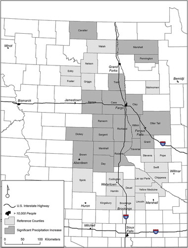
Figure 2. Selected study area counties in the U.S. northern prairie region.

3. Methods and data

To evaluate whether long-term shifts in precipitation and temperature correspond with changes in crop types, we looked at average annual precipitation and monthly growing season temperature during the study period. Annual precipitation data were included to provide a broader perspective on potential multi-year droughts and soil moisture availability for crop use. Only temperature readings from the crop growing season were used as non-growing season data were not relevant. Derived agricultural temperature data such as Crop Heat Units or Growing Degree Days were not calculated as the focus of this analysis was not a detailed accounting of per crop growing conditions. We also looked at a number of human drivers during our study period that most likely contributed to cropping changes. These included the growth of the U.S. corn-based ethanol industry, the rise of U.S. biodiesel production, market prices of U.S. corn and soybeans, changing export markets for soybeans and corn and the transportation system modification to accomplish this trade, changes in both agronomic seed engineering and field practices, modification to U.S. farm policy, and change to the farming culture during the study period. We create a data-based, human driving force narrative that highlights their complexities and reinforces the need to understand such drivers as synergistic collectives. Such collectives, when woven together with biophysical forces, manifest at varied spatial and temporal scales, frequencies, and magnitudes.

3.1. Biophysical data and methods

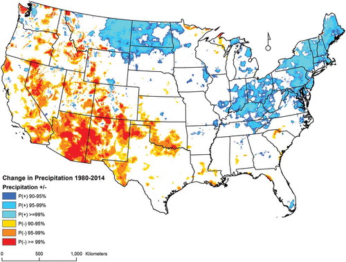
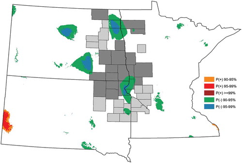
Long-term climate data from Daymet (Thornton et al., 2014) were downloaded for the study area. These data included daily precipitation and temperature from 1980 to 2014. Daymet daily gridded (1 km resolution) precipitation data were summarized into annual precipitation and monthly mean temperature (April through September, 1 km resolution) between 1980 and 2014. The annual precipitation data were used to analyze temporal trends of precipitation across the conterminous United States (CONUS) using linear regression for each data grid. We also conducted t-tests to evaluate significant precipitation trends. Figure 3 illustrates the trends during the study period of mean annual precipitation and associated statistical significance confidence levels across the CONUS. Much of the northern prairie received annual precipitation in amounts greater than the long-term average during the study period (Figure 3). The areal amounts of substantial significant change or only limited to no significant change in annual precipitation between 1980 and 2014 found in Figure 3 were used to select the counties that defined our study area (Figure 2).

Figure 3. Statistical confidence level of change in precipitation (+/increase or – /decrease) from 1980 to 2014 for the conterminous U.S. (Daymet – Thorton et al, 2014).

Annual mean monthly temperature data for the growing season, April through September, were created and then analyzed using linear regression for each Daymet data grid to determine if there had been significant changes to overall growing season temperature during the study period. We conducted t-tests to determine significant inter-annual growing season temperature trends over time, with a zero slope representing the null hypothesis of no trend present. We mapped the results for the three states (North Dakota, South Dakota, and Minnesota) that include the northern prairie.

Research from the plant science literature has indicated that wheat and other small grains can become stressed by higher minimum temperatures during the kernel filling stage of growth. High precipitation during this stage can also result in moisture-based diseases (e.g. Altenbach et al., 2003; Klink, Wiersma, Crawford, & Stuthman, 2014; McMullen, Jones, & Gallenberg, 1997; Peltonen-Sainio, Jauhiainen, & Hakala, 2011). Both instances can result in lower yields or discounted prices for the marketed grain. To investigate if there were potential linkages among higher minimum temperatures, an increase in precipitation, and changes in crop proportions in the region, we analyzed Daymet (1 km grid) minimum temperatures (usually occurring overnight) and total precipitation using monthly averages for June and July (during the kernel filling stage), for regional wheat and other small grains, to determine if there had been significant changes in these variables.

A biophysical characteristic that measures cropping suitability of soils was also analyzed. Crop capability classification data were extracted from the USDA’s gSSURGO soils database (U.S. Dept. of Agriculture 2015a). Data were converted to a 120-meter raster grid and county proportions of each crop capability class were calculated. The county proportions were then aggregated to the county group level. Together, these three general biophysical conditions – inherit soil capability for cropping, typical precipitation amounts, and typical growing season temperatures – form the foundation for what crops can be grown.

3.2 Agricultural data and methods

County-level crop data were obtained from the USDA’s National Agricultural Statistics Service (NASS) annual survey (U.S. Dept. of Agriculture 2015b) and the Census of Agriculture (completed by the U.S. Census Bureau through 1992 and by NASS from 1997 through the rest of our study period). All historical Census of Agriculture through 2002 were available at a single internet location (USDA Census of Agriculture Historical Archive, 2016) whereas the most current iteration, the 2012 Census of Agriculture, was available on the NASS Census of Agriculture website (U.S. Dept. of Agriculture 2016a). The NASS annual survey uses a sample-based methodology designed from several techniques that have long-term geographic stability (U.S. Dept. of Agriculture 2015c) but does not produce measures of uncertainty in area amounts of individual crops for each year. The Census of Agriculture is a long-term episodic enumeration of agricultural production that uses statistical methods to account for non-respondents (U.S. Dept. of Agriculture 2014). The Census of Agriculture also does not give measures of uncertainty of area amounts of individual crops for specific years. With the exception of hay (because there was no alternative choice) data that reflected area planted (instead of area harvested) were used in our analysis to avoid data anomalies caused by droughts or floods.

We analyzed three separate 3-year ‘eras’ evenly spaced across the study period: 1980–1982 (the beginning of the Daymet climatic data and avoiding both the 1983 Payment-In-Kind (PIK) anomaly in general crop planting and the depths of the 1980s farm crisis), 1996–1998 (the introduction of the first genetically modified organism–GMO–soybean and corn seed), and 2011–2013 (generally the post-ethanol boom in the northern prairie region and the end of recent high corn and soybean prices (2007–2012) – drivers often identified as the culprits of recent corn/soy expansion). NASS annual survey data (area planted) were used for most crops for the three eras. Several data gaps occurred in these data that included county level data for all wheat planted after 2007, amount of hay harvested for South Dakota counties in the early 1980s, and area planted for some of the more minor crops. Specific types of wheat (winter, spring, durum) planted were summed to produce the wheat area planted for 2011–2013. Other data gaps were filled with area harvested values from the Census of Agriculture within each specific era (1982, 1997, or 2012). Crop proportions (area planted or harvested) were calculated for each county using the mean of each of the three 3-year eras, and thus representing the 1980 to 2013 study period. To determine whether the aforementioned June and July climatic variables actually affected wheat and several other small grain yields, we compared NASS state-level mean yields for wheat, barley, and oat. This analysis used the three 3-year eras for each of the three states that we included in the northern prairie (U.S. Department of Agriculture, 2015b).

3.3 Spatial change analysis

To effectively analyze the potential impacts of climate variations on crop production, the study area was refined based on annual precipitation change from 1980 to 2014. We selected two groups of counties: those with more than 80% of their territory p ≥ 0.1 positive precipitation trends (‘substantial precipitation increase’ counties) and a control group that had less than 20% of their land area with p ≥ 0.1 positive precipitation trends (‘reference’ counties) (Figure 2). The counties that fell between 20 and 80 percent were not included to determine if the greater percentage spread between the two selected groups made a difference in crop area proportions. The reference counties included those in close geographic-proximity to the counties with substantial significant precipitation increase trends.

In addition to the selected counties within our study area, we also explored whether crop area proportions in the study area were representative of land change across the broader region of North Dakota, South Dakota, and Minnesota using the three 3-year representative eras. The overall area of planted cropland (including harvested hay land) in each state was also examined during each era to assess land-use changes among cropland and other uses, namely land enrolled in CRP. We accomplished this by analyzing the NASS annual survey data at the state level and the area in CRP (from its implementation in 1986 through the end of the study period) using state-level data from the USDA Farm Services Administration agency (U.S. Dept. of Agriculture 2015d). The overall area of land used for the cultivation of major crops and land in CRP allowed us to evaluate several recent conclusions of other studies of land conversion to cropland (e.g. Lark et al., 2015; Wright & Wimberly, 2013) over a longer time span.

3.4 Human drivers and methods

Qualitative methods using available tabular data and a robust literature review were used to assess the impact of human drivers on changing cropping proportions using a narrative approach. In addition, we created spatial databases of ethanol production facilities (initial year of operation and production capacity) and 110-car unit train railroad loading locations and sought expert input from North Dakota county agricultural professionals gathered using standardized e-mail interviews. Information about ethanol facilities was gathered from company websites pertaining to each site whereas the individual locations of unit train loading facilities were found in state transportation databases and through the use of Google Earth™ ‘historical’ imagery slider. Both the coordinates of the ethanol and 110-car unit train loading facilities were entered into GIS software to create maps. The e-mail interviews of county-scale North Dakota crop production experts were conducted in the fall of 2009 and responses were gained from representatives of approximately 15 eastern North Dakota counties.

3.5 Data use at mixed scales and resolutions

The goal of this research was to increase understanding of how changes in human drivers and possible changes in biophysical conditions were intertwined and produced changes in crop proportions in a region where agricultural production trends appeared to be in transition. One of the challenges was integrating data at various scales and resolutions that would help bridge the human-biophysical driving force gap. Researchers in the spatial modeling communities that study land-cover change projections (Bakker & Veldkamp, 2012; Eitelberg, Van Vliet, & Verburg, 2017; Sleeter et al., 2012; Sohl et al., 2016, 2012b, 2012a; Verburg, Veldkamp, & Fresco, 1999; Xia et al., 2017) and carbon fluxes (Liu et al., 2014; Zhao & Liu, 2014) have accepted the integration of multi-scaled data sets and their inherit limitations because other data choices are not available to help answer the complex set of questions such studies attempt to answer (Rinfuss, Walsh, Turner, Fox, & Mishra, 2004; Zhao & Liu, 2014).

4. Results

4.1 Justification for the county groups

The differences in annual precipitation change trends can be seen clearly in the two groups of counties. No county in the substantial precipitation increase trend group had less than a 2-mm/year (Figure 4a) increase and the mean change in annual precipitation for the entire group was 3.86 mm/year during the study period. No individual county in the reference county group had greater than 3-mm/year change (Figure 4b); as a group, the mean change in annual precipitation was relatively stable with a mean of 1.15 mm/year. Both county groups had a significant increase in annual precipitation, although the substantial precipitation increase trend group was much more prominent in change.

Figure 4. Differences in regression slope results of annual precipitation change for individual study area counties, substantial precipitation increase group (4a) and reference counties group (4b).

4.2 Crop proportion changes, comparing cropping capability in the county groups

There were notable changes in mean crop proportions in the group of counties with substantial positive precipitation trends during the study period (Table 1). Wheat was by far the most planted crop in these counties during the early 1980s but lost its predominance during the study period, primarily between the late 1990s and circa 2013. Corn began as part of a second tier of crops, which also included barley and sunflowers, and soybeans were in a third tier with harvested hay and oat. By the middle of the study period, however, soybeans and corn had reached overall second and third place, respectively, behind wheat. Soybeans in particular, in the substantial positive precipitation trend counties, rose substantially from 6th place in the early 1980s to 1st place in area planted by circa 2013. Some minor crops also made gains in mean proportions of area planted such as canola (a Canadian-developed form of rapeseed), sugar beets, and dry beans. Crops that had been prominent in the early 1980s, such as barley and sunflowers, along with more minor small grains, had nearly disappeared by circa 2013. Hay area also declined during the second half of the study period.

Table 1. Crop proportions of land use area found in the substantial precipitation increase counties for the 1980–1982, 1996–1998, and 2011–2013 eras. Totals may not equal 100.0% due to rounding.

Crop Type	1980–1982 mean proportion of area crop land use	Crop Type	1996–1998 mean proportion of area crop land use	Crop Type	2011–2013 mean proportion of area crop land use
Wheat	39.3%	Wheat	35.9%	Soybeans	40.2%
Barley	13.3%	Soybeans	21.9%	Corn	31.9%
Sunflowers	11.9%	Corn	14.0%	Wheat	14.0%
Corn	10.2%	Hay Harvested	7.6%	Hay Harvested	4.5%
Hay Harvested	7.8%	Barley	7.2%	Sugar Beets	2.8%
Soybeans	6.2%	Sunflowers	5.2%	Canola	2.7%
Oat	5.7%	Dry Beans & Peas	2.8%	Dry Beans & Peas	2.1%
Sugar Beets	1.8%	Sugar Beets	2.6%	Barley	0.7%
Flax	1.5%	Canola	1.2%	Sunflowers	0.5%
Dry Beans & Peas	1.2%	Oat	1.1%	Oat	0.3%
Rye	0.8%	Potatoes	0.3%	Potatoes	0.2%
Potatoes	0.3%	Flax	0.2%	Flax	0.1%
Canola	0.0%	Rye	0.2%	Rye	0.0%
Sorghum	0.0%	Sorghum	0.0%	Sorghum	0.0%

In the reference counties, wheat was the leading crop planted during the early 1980s but was replaced by soybeans and corn by the later 1990s (Table 2). Corn remained as one of the leading crops across the entire study period in this group of northern prairie counties but its mean proportion in area planted nearly doubled. Soybeans increased much the same as in the substantial precipitation increase counties to become the second leading crop by the end of the study period. Together, corn and soybeans accounted for three-quarters of the mean proportion of crops planted in the reference counties by circa 2013. Other small grains besides wheat and other oil crops besides soybeans had a secondary presence in this group of counties in the early 1980s but greatly diminished over time. By 2013, corn, soybeans, wheat, and hay were grown on over 90 percent of the cropland in the reference counties.

Table 2. Crop proportions of land use area found in the reference counties for the 1980–1982, 1996–1998, and 2011–2013 eras. Totals may not equal 100.0% due to rounding.

Crop Type	1980–1982 mean proportion of area crop land use	Crop Type	1996–1998 mean proportion of area crop land use	Crop Type	2011–2013 mean proportion of area crop land use
Wheat	30.3%	Soybeans	27.9%	Corn	38.8%
Corn	21.9%	Corn	25.8%	Soybeans	37.3%
Soybeans	11.3%	Wheat	21.5%	Wheat	10.3%
Hay Harvested	9.0%	Hay Harvested	8.7%	Hay Harvested	5.2%
Sunflowers	8.5%	Barley	4.9%	Dry Beans & Peas	3.3%
Oat	8.4%	Sunflowers	4.8%	Sugar Beets	1.7%
Barley	5.6%	Dry Beans & Peas	2.0%	Barley	1.2%
Flax	2.0%	Sugar Beets	1.5%	Canola	0.8%
Potatoes	0.9%	Oat	1.2%	Potatoes	0.6%
Rye	0.8%	Potatoes	0.7%	Oat	0.4%
Sugar Beets	0.8%	Canola	0.4%	Sunflowers	0.3%
Dry Beans & Peas	0.3%	Flax	0.3%	Flax	0.0%
Sorghum	0.2%	Rye	0.2%	Rye	0.0%
Canola	0.0%	Sorghum	0.0%	Sorghum	0.0%

A comparison of the two study groups using USDA gSSURGO soils-based cropping capability data (U.S. Department of Agriculture, 2015a) revealed similarities (Table 3). Cropping capability classes 1 and 2 correspond to soils best suited for cropland (Klingebiel & Montgomery, 1961–see table 3 for details of specific classes). Class 3 has higher erosion potential and lower fertility than classes 1 and 2, but is still often cropped. Classes 1 through 3 totaled 80.8 percent of the reference counties’ area versus 78.1 percent of the substantial precipitation increase group. Most of the leading crops in the northern prairie have a general plasticity for good growth in better soils. Because the results of both groups were so similar we did not run statistical tests of this variable against changes in crop proportions.

Table 3. The substantial precipitation increase counties group land area overall capability of cropping versus reference county group. Cropping capability decreases with higher numbers, numbers 6 through 8 not shown. Overall descriptions of cropping classes found in Klingebriel & Montgomery (1961).

Cropping Capability Class	Overall description of cropping classes	Counties w/Substantial Precipitation Increases	Reference Counties
0		2.7%	2.4%
1	Soils that have few limitations that restrict their use.	3.6%	5.4%
2	Soils that have some limitations that reduce the choice of plants or require moderate conservation practices.	56.6%	56.5%
3	Soils that have severe limitations that reduce the choice of plants or require special conservation practices or both.	17.9%	18.9%
4	Soils that have severe limitations that restrict the choice of plants, require very careful management, or both.	8.6%	7.0%
5	Soils that little or no erosion hazard but have other limitations impractical to remove that limit their use largely to pasture, range, woodland, or wildlife food and cover.	10.6%	9.9%

4.3 Crop proportion changes in the regional states

At the state level, the percentages of harvested hay area decreased less (nearly 25%) using 3-year means of 1980–1982, 1996–1998, and 2011–2013 than in the two groups of study counties (42% in the reference counties and 44% in the substantial precipitation increase counties). This difference may indicate that farmers in the study counties with mostly good soils for cropping could replace hay with other crops, whereas at the state scale, where more overall marginal lands are found, hay may be the only feasible or most profitable crop option (e.g. northern Minnesota or parts of the western Dakotas). The pattern of loss of area planted to non-wheat small grains and sunflowers as part of the ‘other’ category is apparent at the state level (Figure 5). Land planted to oat, barley, and sunflowers decreased approximately 89%, 75%, and 70%, respectively. Corn area substantially increased (+46.5%) but more impressive was the expansion of soybeans, which increased 162.5% during the study period. Together, the area planted to corn and soybeans was approximately 61,566 km² more in circa 2013 in the three states than during the early 1980s. Wheat had the second largest change in overall area planted with a decrease of over 32,000 km². Wheat, along with oat, barley, and sunflowers, provided enough ‘replacement land’ for the observed expansion of corn and soybeans. The area decline in these crops does not indicate, however, that other non-cropland conversions did not also occur.

Figure 5. NASS annual survey area amounts for land planted for the crops listed in Table 1 between 1980 and 2014 and federal Conservation Reserve Program land enrolled 1986–2014 for the combined three states of North Dakota, South Dakota, and Minnesota.

Cropland (the 15 crops found in Table 1) expanded 2.5% from the 1980–1982 mean to the 2011–2013 mean in South Dakota even with 4,377 km² (2011–2013 mean) still part of the CRP (Table 4, U.S. Department of Agriculture, 2015b; U.S. Department of Agriculture, 2015d). South Dakota cropland increased more (5.3%) from the early 1980s if a 2012–2014 mean is used, even though 4,067 km² of CRP remained enrolled. A cold, wet spring in 2011 in North Dakota greatly affected the 2011–2013 cropland area mean value. If a 2012–2014 cropland area mean is used, North Dakota gained just over 2% in cropland area (the 15 crops in Table 1) since the early 1980s with 7,807 km² of CRP land still remaining. Overall, cropland and CRP in the three states peaked in 2008 with 274,387 km² (Figure 5). In comparison, Minnesota cropland in the same crops had a different trajectory than the two other states with a 12% decrease during the study period. Minnesota’s CRP area was between the amounts of the two Dakotas, accounting for part of the ~11,000 km² cropland loss since the early 1980s. However, Minnesota is also the only state of the three that has experienced substantial cropland-to-urban land use conversions. The crop proportion changes found in the selected counties within the study area are similar to the crop proportion change in the entire three state region and, with the exception of Minnesota, more land was in current or recent cropland use (CRP land) at the end of the study period than at the beginning.

Table 4. 3-year means of amount of land used in the 15 studied crops, and CRP land enrolled 1980–1982 (no CRP during this time), 2011–2013, 2012–2014 and percent change. Source: (U.S. Department of Agriculture, 2015b, 2015d) [acres converted to km²].

State	1980–1982 Mean Cropland Used (km^2)	2011–2013 Mean Cropland Used (km^2)	Percent Change from 1980–1982 Mean	2012–2014 Mean Cropland Used (km^2)	Percent Change from 1980–1982 Mean	Enrolled CRP Mean 2011–2013 (km^2)	Enrolled CRP Mean 2012–2014 (km^2)
North Dakota	89,967	84,989	−5.5%	91,822	2.1%	8,977	7,807
South Dakota	67,432	69,122	2.5%	70,978	5.3%	4,377	4,067
Minnesota	91,020	79,687	−12.4%	79,874	−12.2%	6,166	5,713

4.4 Analysis of Changes in Mean Monthly Growing Season Temperature, Minimum Temperature in June and July, and Precipitation in June and July

Our study counties were selected based on whether or not they fell within areas of substantial changes in annual precipitation; we did not know how trends in mean monthly temperature during the growing season would be spatially distributed across the region. A map of p ≥ 0.1 statistical confidence for positive and negative trends in mean monthly temperature for April through September between 1980 and 2014 shows that much of the three states did not experience a significant change in temperature (Figure 6). There were pockets of negative trends in growing season mean temperature that were found in some of our selected counties such as Roberts, SD, Traverse, MN, (both in the substantial positive precipitation trend group) and Walsh, ND (a reference group county). A closer examination of mean crop proportions for these three counties (see Table 5, in Supplemental data) shows that the general patterns found in the two groups of study counties, as well the overall three states, maintained in these pockets of negative trend in mean growing season temperature; the area of corn increased, the areas of wheat, other small grains, and sunflowers decreased, and the area planted to soybeans increased greatly over time.

Figure 6. Statistical confidence level of temperature change (+/increase or – /decrease) in mean growing season (April through September) temperature from 1980 to 2014 for North Dakota, South Dakota, and Minnesota.

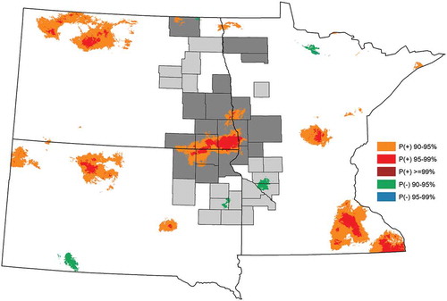
Our examination of temporal changes in minimum temperatures for June and July show quite different results than mean growing season temperature. Areas of positive increases (p ≥ 0.1 confidence intervals) in minimum temperatures for these two months were found across the three states, including much of eastern North Dakota (Figure 7). Changes in positive increases of precipitation in June and July were much more limited in geographical extent (Figure 8). The state-level trends in grain yields, however, do not appear to support the belief that higher minimum temperatures in June and July adversely affected wheat production (see Table 6, in Supplemental data). The mean yield per land unit increased in all three states over the study period using the three 3-year eras. Other small grains yields, such as oat and barley, perhaps were more sensitive to higher minimum temperatures, among other climatic variables, as reported by Klink, Wiersma, Crawford, and Stuthman (2014) for their agricultural-university campus test sites. State-level trends using the three 3-year eras show that whereas oat yields for the Dakotas had greater than 35% increases between the beginning and ending of our study period, oat yields in Minnesota actually showed a 6% decrease (see Table 6, in Supplemental data). Barley yields at the state level, with the exception of North Dakota, showed only an 11–13% increase across time, the lowest of any of the crops found in Table 6. Over time, it also seems unlikely from the limited changes in precipitation in the region for these two months that widespread outbreaks of excessive moisture diseases greatly impacted wheat production, although local and shorter temporal conditions during specific years may be masked by the overall study period length analysis. This was the case when a major small grains ‘scab’ infestation heavily impacted parts of the study area in the excessively wet year of 1993 and several subsequent years (McMullen et al., 1997).

Figure 7. Statistical confidence level of temperature change (+/increase or – /decrease) in mean minimum temperature for June and July from 1980 to 2014 for North Dakota, South Dakota, and Minnesota.

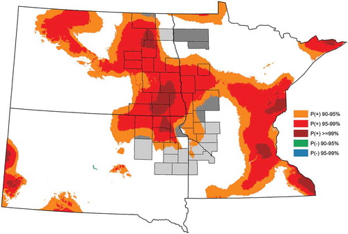
Figure 8. Statistical confidence level of precipitation change (+/increase or – /decrease) for June and July from 1980 to 2014 for North Dakota, South Dakota, and Minnesota.

5. Human drivers of crop area proportion changes in northern prairie

5.1 Introduction to human drivers

Human drivers affect, facilitate, and cause land use change (e.g. Auch, Napton, Kambly, Moreland, & Sayler, 2012; Lambin et al., 2001; Meyer & Turner 1994; Napton et al., 2010). Increased biofuel production and high commodity prices are the oft-cited reasons for increased corn and soybean production in the northern prairie (e.g. Gallant et al. 2014; Graesser, 2008; Johnston, 2014; Lark et al., 2015; Otto et al., 2016; Wright & Wimberly, 2013). Undoubtedly, these drivers have affected crop area proportion changes, but other socioeconomic factors are also involved. Auch et al. (2012) illustrated how a ‘web’ of multiple drivers often merge together in space and time to influence land-use change. Such webs are difficult to quantitatively assess; nonetheless, we examine some of the drivers that have impacted land change on the northern prairie.

5.2 Change in U.S. corn and ethanol production

U.S. corn production steadily increased throughout our study period (Figure 9) with annual variability linked to changes in federal farm programs (e.g. the short-lived 1983 PIK program) or droughts (e.g. 1988, 2012). The U.S. corn crop consumed by the ethanol industry was minimal during the first 20 years of the study period and did not surpass 50 million tonnes (nearly 2 billion bushels) until 2006 (Figure 9, U.S. Dept. of Agriculture 2015e). Corn consumed by ethanol rose to over 127 million tonnes (5 billion bushels) by 2010 where it has since plateaued, declining only slightly during the 2012 drought.

Figure 9. U.S. overall corn and soybean production from 1980 to 2014, as well as corn used for ethanol production, corn used for other industrial uses that do not include direct livestock feed and exports, soybeans used for crush, and soybeans exported.

Sources: (U.S. Department of Agriculture, 2015e; U.S. Dept. of Agriculture 2015f).

Our study area, and slightly beyond, included 19 ethanol production facilities: six in both the substantial precipitation increase counties and reference counties, and an additional seven located within 80 km (50 miles) of the study area. Most were constructed between 2001 and 2006 when U.S. ethanol production was increasing, although the substantial precipitation increase counties had a greater percentage of their facilities built in 2007 and thereafter. The capacity of individual ethanol facilities to use more corn may be the most important attribute to consider. Generally, facilities in the reference counties and just outside of those counties were smaller in size than the facilities within the substantial precipitation increase counties (Figure 10). The reference counties group had only one facility that exceeded 379 million liters (approximately 100 million gallons) of annual production whereas two plants located in the North Dakota substantial precipitation increase counties had equivalent capacities. Ethanol production facilities can also be expanded for greater capacity. The Aberdeen, South Dakota facility, in the substantial precipitation increase group, was established before 2000; by 2017, the addition of a second facility at the same site had increased the capacity by almost 600% (Advanced BioEnergy, 2017).

Figure 10. Annual production capacity of ethanol facilities in the study area.

Source: Renewable Fuels Association (2017), individual facility websites.

5.3 Change in U.S. biodiesel production

Increased soybean production tends to be included in the ‘biofuels’ portion of the cropland expansion narrative. This is problematic because although almost all corn alcohol goes into vehicle fuel, soybean oil has a number of uses other than biodiesel. During the study period, U.S. soybean oil production steadily increased, long before the presence of biodiesel (Figure 11). Only after 2005 did increases in biodiesel appear to add to soybean oil’s increases and the decreases in soybean oil from 2008 to 2010 are reflected in decreases in biodiesel. Canola was a secondary oil source for biodiesel, along with recycled cooking oil and animal fats (Wisner, 2013). The U.S. does not produce much canola but it is Canada’s largest importer (Canola Council of Canada, 2014). Corn oil as a by-product of corn ethanol refining is also developing as a biodiesel feedstock and appears to be on a trend to surpass canola (Martin, 2016; Wisner, 2013).

Figure 11. U.S. soybean oil and biodiesel production from 1980 to 2014. Sources: U.S. Dept. of Agriculture (2015f) [dry measurement converted to wet measurement]; Biodiesel.org (2015).

5.4 Change in U.S. corn and soybean prices

Corn and soybean prices have not mimicked their overall production increases over time. Iowa corn, used here as a bellwether because of its role as one of the leading corn producing states, normalized to an annual price, was between $2.00 and $3.00 per bushel (24.5 kg) during the first 20 years of the study period as corn production increased (Figure 12). Only in 2007 did Iowa corn sustain over $4.00 a bushel for the year during the rapid expansion of national ethanol production driven primarily by changes in federal biofuel policies and increased use of ethanol as an oxygenate for gasoline after MTBE (Methyl tert-butyl ether) was banned (Tiffany, 2009). The price surge continued, spiking during the drought year of 2012 at nearly $7.00 a bushel, and then fell substantially in 2013 and again in 2014. Soybeans had a wider range in annual price for the first two-thirds of the study period ranging between $4.00 and $8.00 a bushel (27.2 kg), breaking the latter price only once before 2007 (Figure 12). As with corn, per bushel soybean prices rose quickly in 2007, stalled in 2009, and peaked in 2012 at over $14.00 before dropping back to $10.00. Whether both of these crops have established a new ‘base price’ higher than pre-2007 trends remains to be seen, especially with normalized annual prices for corn only in the $3.50–3.35 range for 2015 and 2016 (Iowa State Extension, 2017).

Figure 12. The annualized market year price of corn and soybeans per bushel in Iowa from 1980 to 2014.

Source: Iowa State Extension (2017).

It has been argued by Tiffany (2009) that corn prices are now linked to the price of petroleum by 2005 and 2007 federal legislation that demanded more ethanol use in the national gasoline supply. However, Wisner (2014) indicated that a growing corn supply impacted corn prices more than ethanol when the growth in ethanol production mostly ended by 2013; without increased ethanol demand, overall corn supply was a greater driver of the price of corn. Zulauf (2016) also stressed the linkage in the growth of corn supply to corn prices and noted that ethanol’s impact on corn prices between 2006 and 2013 was an anomalous era (fast-growing ethanol demand on corn versus slower than expected growth in corn yields) compared to years before and after national ethanol use expansion.

5.5. Change in U.S. soybean and corn exports

Soybeans differ from corn in that exporting them has become another dominant end-use (Figure 9) while corn exports have never exceeded 20 percent of U.S. total production (Capehart, 2015). In market year 2014, U.S. soybeans used for exports were approximately 48.7 million tonnes, nearly equaling ‘crushed’ soybeans (48.9 million tonnes) which produces soybean meal and oil. By 2012 China had become the largest purchaser of U.S. soybeans (see Table 7, in Supplemental data) and the largest overall buyer globally. The Chinese have also increased their purchases of U.S. corn (see Table 8, in Supplemental data). New and existing grain ports in the Pacific Northwest such as Kalama and Longview, Washington, have undergone construction or expansion (Pacific Northwest Waterways Association, 2015) and have become major points of departure for Chinese-bound soybeans and corn.

State-level exports of soybeans and corn from the Dakotas and Minnesota nest within a national narrative as the value of soybeans destined for export from the three states increased from 919 million dollars in 2000 to 4.316 billion dollars in 2014, with Minnesota ranking 4th in overall export value of this crop, South Dakota 8th and North Dakota 9th (U.S. Dept. of Agriculture 2015g). The value of corn exported from the three states had less of an overall change, increasing from 546 million dollars in 2000 to 1.723 billion in 2014, with Minnesota ranking 4th nationally, South Dakota 6th, and North Dakota 12th in 2014 (U.S. Department of Agriculture, 2015g). Caveats in using these data are 1) that export destinations are not given; soybeans and corn could be going north into Canada, south to the ports of the lower Mississippi, or east to the port of Duluth/Superior on Lake Superior and 2) that the value of these commodities had risen between 2000 and 2014. The higher prices for soybeans and corn, however, does not fully account for the change if the overall value is divided by Iowa-baseline annual prices (Figure 12) for those years. Those annual prices would indicate that the amount of corn and soybeans leaving the three states bound for export would have increased by 50% and 160%, respectively, between 2000 and 2014.

The northern prairie has emerged as the most proximate production region of these two crops, especially soybeans, to the Pacific Northwest ports. That distance advantage and the emerging Chinese market has encouraged the expansion or construction of grain terminals that can accommodate 110-car unit trains that specialize in carrying specific goods, such as crops, for a single destination (Laingen, 2014). Facilities located in the Red River Valley of North Dakota and Minnesota and the counties in west-central Minnesota of the reference county group were built at an earlier date than ones farther west in North and South Dakota (Figure 13) using the date the facilities were first detected using Google Earth ‘historical’ imagery slider. South Dakota has the largest concentration of the most recent unit train railroad loading facilities, with some located even further west than the James River Valley but still accessible within an hour’s drive of the study area.

Figure 13. The year of construction or expansion of railroad loading facilities that can accommodate 110-car unit trains within an 80 km drive of the study area.

Sources: state transportation systems information or as first detected with Google Earth imagery

5.6 Change in corn and soybean agronomics

Other human-centric driving forces that result in crop area proportion change, such as agronomic advances that alter or improve plant cultivars that may be proprietary, may not be as apparent to those searching geographic or land change literature. Agricultural production experts in North Dakota stated that faster-maturing corn hybrids have existed for quite some time, but yields tended to be low and thus not economically competitive with wheat (USDA-North Dakota crop production experts, email correspondence, 2009). However, yields of such hybrids have improved to the point where they now can compete with wheat and other non-corn/soy crops, and as such, farmers have increased the amount of corn they grow (USDA-North Dakota crop production experts, email correspondence, 2009). Improved agronomics for both corn and soybeans, in both seed genetics and cultivation practices, have allowed them to be produced in areas once thought to be out of their natural range, with some seed companies planning to expand former boundaries even further (Gilmour, 2016). Lee and Tracy (2009) indicated that by the middle of the study period there was full integration between genetic research and current agronomic field practices that resulted in more customized seed choices for producers. Clay et al. (2014) stated that soil health was generally better, at least in the South Dakota counties, later in the study period as management practices that enhanced soil, such as conservation tillage, became more widely used. Other important agronomic strides were changes in crop genetics, especially the introduction of GMO varieties in the late 1990s. By the last of our 3-year eras circa 2013, the ‘stacking’ of GMO traits, such as in corn rootworm (Diabrotica spp.) and corn borer (Ostrinia nubilalis) resistance (both major pests), and glyphosate-resistance, had become standard options when purchasing seed (Johnson & McCuddin, 2009). Advanced seed coatings, especially for corn, introduced other anti-biologics that helped seed survive germination in soil temperature and wetness situations that would have been marginal for success in the past (Stoll & Saab, 2015).

5.7 Change in U.S. farm policy

Other non-biofuel changes to U.S. farm policy also played a role in crop selection choices on the northern prairie. Modern government-subsidized crop insurance began in the early 1980s (U.S. Dept. of Agriculture 2016b). Gradual modifications to this type of insurance guaranteed more revenue protection in later eras of the study period and allowed producers to take more risks in selecting the crops they chose to produce. The 1996 farm bill, referred to as the ‘Freedom to Farm’ act, allowed farmers to plant different crops than in previous years, a change that decoupled substantial portions of farm program payments from production decisions (Babcock & Carriquiry, 2001). This meant that producers no longer had to plant what they had historically planted in order to be eligible to receive government payments and crop insurance. By planting new crops, farmers established ‘APHs’ (actual production histories) and could enter into crop insurance programs. Farmers were now free to plant the crops that would yield them the highest returns (Babcock & Carriquiry, 2001). Thus, synergistic conditions between various aspects in federal farm policy helped establish a new foundation of crop proportions in the region.

5.8 Change in U.S. farm culture

‘The Farm of today, as in the past, is overwhelmingly a business that is owned by the family which lives there and operates it’ (Hudson & Laingen, 2016, 7). The shift from feed grains and livestock to cash-crop farming coincided with a widespread adoption of technology and computerization by farmers (Hart & Lindberg, 2014). There is no simple answer to why this transition occurred, but one cause has been a doubling in world trade in food and feed grains over the past half-century (Raup, 2002). Whereas in the past farmers were concerned only about their operation, modern farmers must be in tune with global patterns of production and consumption that are driven largely by today’s globalized economy (Pechlaner & Otero, 2010).

Starting in the first half of the 20th century and accelerating in more recent decades, corn and soybeans have proven more versatile in creating products than wheat and other small grains (Langreth & Herper, 2009; Pollan, 2006). Overall, neoliberal globalization starting in the 1970s helped concentrate agrifood systems where fewer corporations controlled much of the buying, processing, and selling of agricultural commodities and processing them into finished consumer products (Bonanno, 2014; Constance, Hendrickson, Howard, & Hefferan, 2014). Concentrated corporate control over crop seed production followed suit, especially with the introduction of transgenic varieties (Constance et al., 2014; Langreth & Herper, 2009). The more aggressive genetic manipulation of corn and soybeans was justified because these crops were rarely fed directly to humans, and farmers often found these changed crops more reliable and revenue-generating to grow, as one North Dakota farmer stated, ‘wheat and barley haven’t kept up with the times’ (Langreth & Herper, 2009).

Contemporary farms (e.g. corn/soy, small-grain, or those focused on livestock), while still predominantly family-owned and operated, focus on specialization, in part, because of the massive shift in the costs of production. With seven of ten farms having disappeared since the 1930s, land ownership has changed drastically. Per 0.4-ha (acre) cropland prices regularly exceed $5,000–10,000; annual inputs can be tens-of-thousands of dollars; and large equipment can cost hundreds-of-thousands of dollars. When considering the low cost per unit measurement that farmers receive for what they grow, the amount of land each farm needs to operate are orders of magnitude larger than their mid-20th century counterparts. Hart (2003b) estimated that a modern Midwestern family farm must generate a gross income of at least $250,000 to provide an acceptable level of living for a contemporary American family (where no off-farm income was taken into consideration). To amass such an income, a farmer would need to operate at least 405 ha (1,000 acres), what Hart and Lindberg (2014) call a ‘kilofarm’.

A less-easily quantifiable cultural shift involves the continuation of farm legacies. Many of this region’s farmers grew small grains and raised cattle because that was their family’s farming practice. Much to the consternation of older farmers, a new technologically and economically savvy generation has decided to alter such longstanding land-use and production practices (Hudson & Laingen, 2016). Specialization has helped to create distinct regions where farmers focus their efforts on producing higher-yielding crops while using fewer inputs (e.g. nitrogen) and improved environmental practices (e.g. tillage/residue management, variable-rate fertilizer/chemical application) (Auch & Laingen, 2015). The transition, from more farms with a greater diversity of production to fewer farms with increased specialization, has been ongoing for a century, and will undoubtedly continue into the foreseeable future. Unless drastic changes in domestic and global agricultural consumption trends occur, American farmers will continue to focus on increased specialization to help them maximize yields of the commodities that they raise.

6. Discussion and conclusions

Land change on the northern prairie is complex. Simplistic treatments that cite increased ethanol fuel production and high commodity prices ignore what longer-term and more robust contexts provide to the broader narrative. Fausti (2015) argued ‘ethanol led to more corn’ but also cited the introduction of GMO corn traits in the late 1990s as having played a major role in the increase in corn area planted. Corn, however, had already begun replacing oat and barley in this region before this time (Figure 5) and GMO corn does not explain the rise in soy production between the first two ‘eras’ in this current study. In 1995, the year before any GMO corn or soybeans were sold, farmers in the three states, when answering the NASS annual survey, indicated they would plant 17,886 km² more soybeans than they did in 1980. Our findings reinforce what Wright and Wimberly (2013) and Lark et al. (2015) stated about land conversion on the northern prairie, but also challenge the results of these prior studies by introducing a longer historical record. Our findings indicate that the vast majority (90%+) of the land used to grow these 15 crops circa 2013 was already being used for cropland in the early 1980s, and that recent conversion of natural grassland and wetland provides only a small percentage of currently cropped land.

While our discussion of the human drivers that helped bring about crop proportion changes is admittedly incomplete, it highlights how multiple factors – occurring at varying but usually overlapping spatial and temporal scales – come together to facilitate land change. How human drivers coalesce with biophysical conditions creates an even more complex narrative of how and why land change occurs. Statistical analyses of biophysical drivers (annual precipitation and mean growing season temperature) indicate that increases in annual precipitation were spatially more widespread than changes in mean growing season (April through September) temperature during the study period. These results support responses from agricultural production experts in North Dakota (USDA-North Dakota crop production experts, email correspondence, 2009). Several respondents mentioned how frequent, above average precipitation episodes in the early1990s enhanced moisture-driven disease that affected small grain profitability. Conversely, corn generally benefited from the additional rain. Although many of the surveyed experts stated that corn and soybeans had simply become the more lucrative crops to grow, several perceived that the price dockage for poorer quality small grains caused by excess wetness was a substantial factor persuading farmers to curtail or lessen their planting of small grains (USDA-North Dakota crop production experts, email correspondence, 2009). The overall trend in less small grain planted by area, however, transcended the substantial precipitation increase counties and indicates the interactions of more drivers in their decline than just moldy or lightweight grain.

One of the conclusions from this investigation is that a more robust and extensive survey of producers or crop production experts is needed to further understand the variety of factors contributing to crop type planning by farmers. They are weighing immediate site factors (land productivity), personal financial situation (e.g. will the investment in precision agriculture technology to maximize new seed technology pay off in the few years left remaining to farm?), macro-economic crop markets (forecast prices, foreign production, trade, domestic usage), federal agriculture policy, current biophysical trends (precipitation, temperature conditions), level of personal knowledge, risk management/aversion strategies, and other considerations (MacDonald, Korb, & Hoppe, 2013). Much of the decision making in production agriculture is managing short- and long-term financial risk (Coble & Dismukes, 2008; Hudson & Laingen, 2016). Understanding how observed biophysical changes and anticipated future changes interact with the host of other farm-planning drivers would help provide insight into which agricultural risks are driving production decisions and when.

A second conclusion is that unravelling the complexity typically involved in understanding land change driving forces often presents a conundrum for researchers. Quantitative, statistical analyses are preferred, yet data may not always be available for important drivers that may help form the synergistic web that often facilitates land change. Further, results gleaned from hybrid quantitative-qualitative methods may easily bias the importance of statistical (quantitative) findings and understate what might be more or just as important, but less justifiable, qualitative narratives. Land change researchers have often oversimplified complex stories of land change because they focused on easily quantifiable factors instead of more expansive (albeit less straightforward and more confounding) list of potential/actual drivers. Robust, statistical analyses also do not necessarily compensate for a less quantifiable but more comprehensive knowledge base of regional or thematic land use observations that include larger geographical and historical contexts. Land change modelers have noted, ‘An understanding of land use dynamics requires a deep understanding of a variety of biophysical and socioeconomic processes that occur across a wide range of spatiotemporal and sociopolitical scales’ (Bennet, Tang, & Wang, 2011, 211).

The breadth and complexity of human and biophysical driving force webs often lessens our ability to fully explain resulting land use changes adequately. We partitioned our study area based on precipitation values to explore whether this factor alone was a substantial enough driver to cause crop proportions to change on the northern prairie. When comparing counties that experienced increased precipitation to a set of nearby reference counties, as well as analyzing data at a three-state scale, the increase of corn and soybeans and decreases in small grains and sunflowers was ubiquitous throughout. The last of our conclusions is that increases in annual precipitation did not cause farmers to change their cropping proportions in the U.S. northern prairie; rather, change in such biophysical factors, along with myriad socioeconomic influences – some more obvious than others – tended to manifest themselves at multiple spatial and temporal scales, and thus facilitated change. Humans and the land are dynamic, and the complex web of driving forces that lead to land-use change necessitates the need for ongoing land change studies.

Acknowledgement

The authors would like to thank the U.S. Geological Survey’s Climate and Land Use Change, Climate and Land Use Research and Development Program for support of this research. The authors would also like to thank Jochum Wiersma, University of Minnesota and Joel Ransom, North Dakota State University for helpful suggestions that improved our understanding about small grains growing conditions in the region. The authors also thank Jennifer Rover and Sandra Poppenga, USGS Earth Resources Observation and Science Center and three anonymous reviewers for helpful comments and critiques that improved this paper. Any use of trade, firm, or product names is for descriptive purposes only and does not imply endorsement by the U.S. Government.

Disclosure statement

No potential conflict of interest was reported by the authors.

Supplemental data

Supplemental data for this article can be accessed here.

References

- Advanced BioEnergy. (2017). Aberdeen. Retrieved from http://advancedbioenergy.com/locations_aberdeen.htm
- Altenbach, S.B., Dupont, F.M., Kothari, M., Chan, R., Johnson, E.L., & Lieu, D. (2003). Temperature, water, and fertilizer influence the timing of key events during grain development in a US spring wheat. Journal of Cereal Science, 37, 9–20. doi:10.1006/jcrs.2002.0483
- Auch, R.F. (2015). Chapter 7 Northern Glaciated Plains Ecoregion. J.L. Taylor, W. Acevedo, R.F. Auch, & M.A. Drummond (Eds.), Status and Trends of Land Change in United States Great Plains—1973 to 2000 (pp. 69–76). U.S. Geological Survey Professional Paper 1794-B. Retrieved from http://pubs.er.usgs.gov/publication/pp1794B
- Auch, R.F., & Laingen, C. (2015). Having it both ways? land use change in a U.S. midwestern agricultural ecoregion. The Professional Geographer, 67(1), 84–97. doi:10.1080/00330124.2014.921015
- Auch, R.F., Napton, D.E., Kambly, S., Moreland, T.R., Jr., & Sayler, K.L. (2012). The driving forces of land change in the northern piedmont of the United States. Geographical Review, 102(1), 53–75. doi:10.1111/gere.2012.102.issue-1
- Babcock, B., & Carriquiry, M. (2001). Acreage shifts under freedom to farm. Iowa Ag Review, 7(1), 4–5.
- Bakker, M., & Veldkamp, A. (2012). Changing relationships between land use and environmental characteristics and their consequences for spatially explicit land-use change prediction. Journal of Land Use Science, 7(4), 407–424. doi:10.1080/1747423X.2011.595833
- Beck, J., & Wright-Knoll, P. (2000). Soil Survey of Marshall County, Minnesota, Part I (pp. 149). Natural Resources Conservation Service, USDA. Washington, D.C.: U.S. Government Printing Office.
- Bennett, D.A., Tang, W., & Wang, S. (2011). Toward an understanding of provenance in complex land use dynamics. Journal of Land Use Science, 6(2–3), 211–230. doi:10.1080/1747423X.2011.558598
- Biodiesel.org. 2015. Production statistics. Retrieved from http://biodiesel.org/production/production-statistics
- Bogue, D.J., & Beale, C.L. (1961). Economic Areas of the United States (pp. 1161). New York, NY: The Free Press of Glencoe.
- Bonanno, A. (2014). Agriculture and food in the 2010s. In C. Bailey, L. Jensen, & E. Ransom (Eds.), Rural America in a Globalizing World Problems and Prospects for the 2010s (pp. 3–15). Morgantown, WV: West Virginia University Press.
- Brooks, M.S. (2015). Chapter 6 Lake Agassiz Plain Ecoregion. J.L. Taylor, W. Acevedo, R.F. Auch, & M.A. Drummond (Eds.), Status and trends of land change in United States Great Plains—1973 to 2000 (pp. 61–67). U.S. Geological Survey Professional Paper 1794-B. Retrieved from http://pubs.er.usgs.gov/publication/pp1794B
- Bryce, S.A., Omernik, J.M., Pater, D.E., Ulmer, M., Schaar, J., Freeouf, J., … Azevedo, S.H. (1998). Ecoregions of North and South Dakota. U.S. Geological Survey Ecoregion Map Series, scale 1:500,000. Retrieved from http://www.epa.gov/wed/pages/ecoregions/ndsd_eco.htm.
- Canola Council of Canada. (2014). Industry overview. Retrieved from http://www.canolacouncil.org/markets-stats/industry-overview/
- Capehart, T. (2015). Corn–Background. U.S. Dept. of Agriculture, Economic Research Service. Retrieved from http://www.ers.usda.gov/topics/crops/corn/background.aspx.
- Carpenter, S.R., Booth, E.G., Gillon, S., Kucharik, C.J., Loheide, S., Mase, A.S., … Wardropper, C.B. (2015). Plausible futures of a social-ecological system: Yahara watershed, Wisconsin, USA. Ecology and Society, 20(2), 10. doi:10.575/ES-07433_200210
- Chase, T.N., Pielke, R.A., Sr., Kittel, T.G.F., Baron, J.S., & Stohlgren, T.J. (1999). Potential impacts on Colorado Rocky Mountain weather due to land use changes on the adjacent Great Plains. Journal of Geophysical Research Atmospheres, 104(D14). art. no. 1999JD900118, 16673-16690. doi:10.1029/1999JD900118
- Clay, D.E., Clay, S.A., Reitsma, K.D., Dunn, B.H., Smart, A.J., Carlson, G.G., … Stone, J.J. (2014). Does the conversion of grasslands to row crop production in semi-arid areas threaten global food supplies? Global Food Security, 3, 22–30. doi:10.1016/j.gfs.2013.12.002
- Coble, K.H., & Dismukes, R. (2008). Distributional and risk reduction effects of commodity revenue program design. Review of Agricultural Economics, 30(3), 543–553. doi:10.1111/raec.2008.30.issue-3
- Conniff, R. (2012). When civilizations collapse. environment Yale, School of Forestry and Environmental Studies. Retrieved from http://environment.yale.edu/envy/stories/when-civilizations-collapse/.
- Constance, D.H., Hendrickson, M., Howard, P.H., & Hefferan, W.D. (2014). Economic concentration in the agrifood system: Impacts on rural communities and emerging responses. In C. Bailey, L. Jensen, & E. Ransom (Eds.), Rural America in a globalizing world problems and prospects for the 2010s (pp. 16–35). Morgantown, WV: West Virginia University Press.
- Czech, B., Krausman, P.R., & Devers, P.K. (2000). Economic associations among causes of species endangerment in the United States. BioScience, 50(7), 593–601. doi:10.1641/0006-3568(2000)050[0593:EAACOS]2.0.CO;2
- Drummond, M.A., Auch, R.F., Karstensen, K.A., Sayler, K.L., Taylor, J.L., & Loveland, T.R. (2012). Land change variability and human-environment dynamics in the United States Great Plains. Land Use Policy, 29(3), 710–723. doi:10.1016/j.landusepol.2011.11.007
- Eitelberg, D.A., Van Vliet, J., & Verburg, P.H. (2017). Accounting for monogastric livestock as a driver in global land use and cover change assessments. Journal of Land Use Science, 12(1), 1–16. doi:10.1080/1747423X.2016.1270361
- Fausti, S.W. (2015). The causes and unintended consequences of a paradigm shift in corn production practices. Environmental Science & Policy, 52, 41–50. doi:10.1016/j.envsci.2015.04.017
- Gage, A.M., Olimb, S.K., & Nelson, J. (2016). Plowprint: Tracking cumulative cropland expansion to target grassland conservation. Great Plains Research, 26, 107–116. doi:10.1353/gpr.2016.0019
- Gallant, A.L., Euliss, Jr., N.H., & Browning, Z. (2014). Mapping large-area landscape suitability for honey bees to assess the influence of land-use change on sustainability of national pollination services. Plos One, 9(6), 1–14.
- Gilmour, G. (2016). The Corn Belt moves north Monsanto has plans to produce varieties that can be grown on half the acres in western Canada. Country Guide, March 8. Retrieved from https://www.country-guide.ca/2016/03/08/the-corn-belt-moves-north/48412/
- Graesser, J. (2008). The Impact of Ethanol on Land Use in the Northwestern Corn Belt. Brookings, SD: South Dakota State University, Dept. of Geography, Master Thesis.
- Gude, P.H., Hansen, A.J., Rasker, R., & Maxwell, B. (2006). Rates and drivers of rural residential development in the Greater Yellowstone. Landscape and Urban Planning, 77(1–2), 131–151. doi:10.1016/j.landurbplan.2005.02.004
- Hart, J.F. (2001). Half a century of cropland change. Geographical Review, 91(3), 525–543. doi:10.2307/3594739
- Hart, J.F. (2003a). Specialty cropland in California. Geographical Review, 93(2), 153–170. doi:10.1111/j.1931-0846.2003.tb00027.x
- Hart, J.F. (2003b). The changing scale of American agriculture. Charlottesville, VA: University of Virginia Press.
- Hart, J.F., & Lindberg, M.B. (2014). Kilofarms in the agricultural heartland. The Geographical Review, 104(2), 139–152. doi:10.1111/gere.2014.104.issue-2
- Hudson, J.C. (1994). Making the Corn Belt (pp. 254). Bloomington, IN: University of Indiana Press.
- Hudson, J.C., & Laingen, C.R. (2016). American farms, american food: A geography of agriculture and food production in the United States (pp. 158). Lanham, MD: Lexington Books.
- Hupp, C.R., Noe, G.B., Schenk, E.R., & Benthem, A.J. (2013). Recent and historic sediment dynamics along Difficult Run, a suburban Virginia piedmont stream. Geomorphology, 180–181(2013), 156–169. doi:10.1016/j.geomorph.2012.10.007
- Iowa State Extension. (2017). Iowa Cash Corn and Soybean Prices. Retrieved from http://www.extension.iastate.edu/agdm/crops/pdf/a2-11.pdf.
- James, L.A. (2011). Contrasting geomorphic impacts of pre- and post-columbian land-use changes in Anglo America. Physical Geography, 32(5), 399–422. doi:10.2747/0272-3646.32.5.399
- Jelinek, L.J. (1979). Harvest Empire a History of California Agriculture (pp. 113). San Francisco, CA: Boyd and Fraser Publishing Company.
- Johnson, G.R., & McCuddin, Z.P. (2009). Maize and the biotech industry. In J.L. Bennetzen & S. Hake (Eds.), Handbook of Maize Genetics and Genomics (pp. 115–135). New York, NY: Springer.
- Johnston, C.A. (2014). Agricultural expansion: Land use shell game in the U.S. northern plains. Landscape Ecology, 29(1), 81–95. doi:10.1007/s10980-013-9947-0
- Kim, H.W., Amalya, D.M., Chescheir, G.M., Skaggs, W.R., & Nettles, J.E. (2013). Hydrologic effects of size and location of fields converted from drained pine forest to agricultural cropland. Journal of Hydrologic Engineering, 18(5), 552–566. doi:10.1061/(ASCE)HE.1943-5584.0000566
- Klingebiel, A.A., & Montgomery, P.H. (1961). Land-Capability Classification. Washington, DC: U.S. Government printing Office, U.S. Department of Agriculture, Soil Conservation Service, Agriculture Handbook No. 210. Retrieved from http://www.nrcs.usda.gov/Internet/FSE_DOCUMENTS/nrcs142p2_052290.pdf)
- Klink, K., Wiersma, J.J., Crawford, C.J., & Stuthman, D.D. (2014). Impacts of temperature and precipitation variability in the northern plains of the United States and Canada on the productivity of spring barley and oat. International Journal of Climatology, 34, 2805–2818. doi:10.1002/joc.3877
- Laingen, C.R. (2014). A picture is worth 898 words: Changing agricultural landscapes of the Dakotas. FOCUS on Geography, 57(1), 41–42. doi:10.1111/foge.2014.57.issue-1
- Lambin, E.F., Turner, B.L., Geist, H.J., Agbola, S.B., Angelsen, A., Bruce, J.W., … Xu, J. (2001). The causes of land-use and land-cover change: Moving beyond the myths. Global Environmental Change, 11(4), 261–269. doi:10.1016/S0959-3780(01)00007-3
- Langreth, R., & Herper, M. (2009, December 31). The planet versus Monsanto. Forbes, Retrieved from https://www.forbes.com/forbes/2010/0118/americas-best-company-10-gmos-dupont-planet-versus-monsanto.html
- Lark, T.J., Mueller, R.M., Johnson, D.M., & Gibbs, H.K. (2017). Measuring land-use and land-cover change using the U.S. department of agriculture’s cropland data layer: Cautions and recommendations. International Journal of Applied Earth Observation and Geoinformatics, 62, 224–235. doi:10.1016/j.jag.2017.06.007
- Lark, T.J., Salmon, J.M., & Gibbs, H.K. (2015). Cropland expansion outpaces agricultural and biofuel policies in the United States. Environmental Research Letters, 10, 044003. doi:10.1088/1748-9326/10/4/044003
- Lee, E.A., & Tracy, W.F. (2009). Modern maize breeding. In J.L. Bennetzen & S. Hake (Eds.), Handbook of Maize Genetics and Genomics (pp. 141–160). New York, NY: Springer.
- Levers, C., Butsic, V., Verburg, P.H., Müller, D., & Kuemmerle, T. (2016). Drivers of changes in agricultural intensity in Europe. Land Use Policy, 58, 380–393. doi:10.1016/j.landusepol.2016.08.013
- Liu, S., Liu, J., Wu, Y., Young, C.J., Werner, J.M., Dahal, D., Oeding, J., & Schmidt, G.L. (2014). Chapter 7 Baseline and projected future carbon storage and greenhouse-gas fluxes in terrestrial ecosystems of the eastern United States. In Z. Zhu & B.C. Reed (Eds.), Baseline and projected future carbon storage and greenhouse-gas fluxes in ecosystems of the Eastern United States (pp. 115–177). U.S. Geological Survey Professional Paper 1804. Retrieved from http://pubs.usgs.gov/pp/1804/pdf/pp1804.pdf.
- Liu, S., Tan, Z., Li, Z., Zhao, S., & Yuan, W. (2011). Are soils of Iowa USA currently a carbon sink or source? Simulated changes in SOC stock from 1972 to 2007. Agriculture, Ecosystems & Environment, 140, 106–112. doi:10.1016/j.agee.2010.11.017
- Lotze-Campen, H. (2011). Climate change, population growth, and crop production: An overview. In S.S. Yadev, R.J. Redden, J.L. Hatfield, H. Lotze-Campen, & A.E. Hall (Eds.), Crop adaptation of climate change (pp. 1–11). Chichester, UK: John Wiley & Sons.
- MacDonald, J.M., Korb, P., & Hoppe, R.A. (2013). Farm Size and the Organization of U.S. Crop Farming. Dept. of Agriculture, Economic Research Service, ERR-152. Retrieved from: https://www.ers.usda.gov/webdocs/publications/45108/39359_err152.pdf?v=41526
- Marshall, C.H., Pielke, R.A., Sr., & Steyaert, L.T. (2003). Wetlands: Crop freezes and land-use change in Florida. Nature, 426(6962), 29–30. doi:10.1038/426029a
- Martin, J. 2016. Everything you wanted to know about biodiesel (charts and graphs included!). June 22. Union of Concerned Scientists. Retreived from http://blog.ucsusa.org/jeremy-martin/all-about-biodiesel
- McMullen, M., Jones, R., & Gallenberg, D. (1997). Scab of wheat and barley: A re-emerging disease of devastating impact. Plant Disease, 81(12), 1340–1348. doi:10.1094/PDIS.1997.81.12.1340
- Meiyappan, P., Dalton, M., O’Neill, B.C., & Jain, A.K. (2014). Spatial modeling of agricultural land use change at global scale. Ecological Modelling, 291, 152–174. doi:10.1016/j.ecolmodel.2014.07.027
- Meyer, S.R., Johnson, M.L., Lilleholm, R.J., & Cronan, C.S. (2014). Development of a stakeholder-driven spatial modeling framework for strategic landscape planning using Bayesian networks across two urban-rural gradients in Maine, USA. Ecological Modelling, 291, 42–57. doi:10.1016/j.ecolmodel.2014.06.023
- Meyer, W.B., & Turner II, B.L. (Eds.). (1994). Changes in land use and land cover: A global perspective (pp. 549). New York, NY: Cambridge University Press.
- Napton, D., & Graesser, J. (2011). Agricultural land change in the northwestern corn belt, usa: 1972-2007. Geo-Carpathica, 11(11), 65–81.
- Napton, D.E., Auch, R.F., Headley, R., & Taylor, J.L. (2010). Land changes and their driving forces in the southeastern United States. Regional Environmental Change, 10(1), 37–53. doi:10.1007/s10113-009-0084-x
- Newman, S.M., Carroll, M.S., Jakes, P.J., & Pavegilo, T.B. (2013). Land development patterns and adaptive capacity for wildfire: Three examples from Florida. Journal of Forestry, 111(3), 167–174. doi:10.5849/jof.12-066
- Omernik, J.M. (1987). Ecoregions of the conterminous United States. Annals of the Association of American Geographers, 77(1), 118–125. doi:10.1111/j.1467-8306.1987.tb00149.x
- Otto, C.R.V., Roth, C.L., Carlson, B.L., & Smart, M.D. (2016). Land-use change reduces habitat suitability for supporting managed honey bee colonies in the Northern Great Plains. Proceedings of the National Academy of Science, 113, 10430–10435. doi:10.1073/pnas.1603481113
- Pacific Northwest Waterways Association. (2015). Impacts of channel deepening on the Columbia River. Retrieved from http://www.pnwa.net/wp-content/uploads/2012/11/Channel-Deepening-Report-6-18-2015.pdf.
- Pechlaner, G., & Otero, G. (2010). The neoliberal food regime: Neoregulation and the new division of labor in North America. Rural Sociology, 75(2), 179–208. doi:10.1111/j.1549-0831.2009.00006.x
- Peltonen-Sainio, P., Jauhiainen, L., & Hakala, K. (2011). Crop response to temperature and precipitation according to long-term multi-location trials at high-latitude conditions. The Journal of Agricultural Science, 149, 49–62. doi:10.1017/S0021859610000791
- Pollan, M. (2006). The Omnivore’s Dilemma: A natural history of four meals (pp. 450). New York: The Penguin Press.
- Power, A.G. (2010). Ecosystem services and agriculture: Tradeoffs and synergies. Philosophical Transactions of the Royal Society B: Biological Sciences, 365(1554), 2959–2971. doi:10.1098/rstb.2010.0143
- Prince, H. (1997). Wetlands of the American midwest a historical geography of changing attitudes (pp. 410). Chicago, IL: The University of Chicago Press.
- Raup, P.M. (2002). Reinterpreting structural changes in U.S. agriculture. In M. Canavari, P. Caggiati, & K.W. Easter (Eds.), Economic studies on food, agriculture, and the environment (pp. 185–200). New York: Kluwer Academic/Plenum Publishers.
- Renewable Fuels Association. (2017). Biorefinery locations. Retrieved from http://www.ethanolrfa.org/resources/biorefinery-locations/.
- Rinfuss, R.R., Walsh, S.J., Turner II, B.L., Fox, J., & Mishra, V. (2004). Developing a science of land change: Challenges and methodological issues. Proceedings of the National Academy of Sciences, 101(39), 13976–13981. doi:10.1073/pnas.0401545101
- Schaefer, W.T., Jr. (2005). Soil survey of brookings county, South Dakota (pp. 379). Natural Resources Conservation Services, USDA. Washington, D.C.: U.S. Government Printing Office.
- Schwarz, H.E., Jacque, E., Dickens, W.J., Rogers, P., & Thompson, J. (1990). Water quality and flows. In B.L. Turner II, W.C. Clark, R.W. Kates, J.F. Richards, J.T. Mathews, & W.B. Meyer (Eds.), The Earth as transformed by human action (pp. 253–270). Cambridge, UK: Cambridge University Press.
- Serra, P., Pons, X., & Sauri, D. (2008). Land-cover and land-use change in a Mediterranean landscape: A spatial analysis of driving forces integrating biophysical and human factors. Applied Geography, 28(3), 189–209. doi:10.1016/j.appgeog.2008.02.001
- Sleeter, B., Sohl, T., Bouchard, M., Reker, R., Soulard, C., Acevedo, W., … Zhu, Z. (2012). Scenarios of land use and land cover change in the conterminous United States—Utilizing the special report on emission scenarios at ecoregional scales. Global Environmental Change, 22(4), 896–914. doi:10.1016/j.gloenvcha.2012.03.008
- Smaliychuk, A., Müller, D., Prishchepov, A.V., Levers, C., Kruhlov, I., & Kuemmerle, T. (2016). Recultivation of abandoned agricultural lands in Ukraine: Patterns and drivers. Global Environmental Change, 38, 70–81. doi:10.1016/j.gloenvcha.2016.02.009
- Sohl, T.L., Loveland, T.R., Sleeter, B.M., Sayler, K.L., & Barnes, C.A. (2010). Addressing foundational elements of regional land-use change forecasting. Landscape Ecology, 25(2), 233–247. doi:10.1007/s10980-009-9391-3
- Sohl, T.L., Reker, R., Bouchard, M., Sayler, K., Dornbierer, J., Wika, S., … Friesz, A. (2016). Modeled historical land use and land cover for the conterminous United States. Journal of Land Use Science, 11(4), 476–499. doi:10.1080/1747423X.2016.1147619
- Sohl, T.L., Sayler, K.L., Drummond, M.A., & Loveland, T.R. (2007). The FORE-SCE model: A practical approach for projecting land cover change using scenario-based modeling. Journal of Land Use Science, 2(2), 103–126. doi:10.1080/1747423071218202
- Sohl, T.L., Sleeter, B.M., Sayler, K.L., Bouchard, M.A., Reker, R.R., Bennett, S.L., … Zhu, Z. (2012b). Spatially explicit land-use and land-cover scenarios for the Great Plains of the United States. Agriculture, Ecosystems & Environment, 153, 1–15. doi:10.1016/j.agee.2012.02.019
- Sohl, T.L., Sleeter, B.M., Zhu, Z., Sayler, K.L., Bennett, S., Bouchard, M., … Acevedo, W. (2012a). A land-use and land-cover modeling strategy to support a national assessment of carbon stocks and fluxes. Applied Geography, 34, 111–124. doi:10.1016/j.apgeog.2011.10.019
- Soulard, C.E., & Wilson, T.S. (2015). Recent land-use/land-cover change in the Central California Valley. Journal of Land Use Science, 10(1), 59–80. doi:10.1080/1747423X.2013.841297
- Stoll, M., & Saab, I. (2015). Soil temperature and corn emergence. DuPont, Pioneer Retrieved from https://www.pioneer.com/home/site/us/agronomy/soil-temp-corn-emergence/
- Tan, Z., Liu, S., Johnston, C.A., Loveland, T.R., Tieszen, L.L., Liu, J., & Kurtz, R. (2005). Soil organic carbon dynamics as related to land use history in the northwestern Great Plains. Global Biogeochemical Cycles, 19, GB3011. doi:10.29/2005GB002536
- Thompson, J.R., Foster, D.R., Scheller, R., & Kittredge, D. (2011). The influence of land use and climate change on forest biomass and composition in Massachusetts, USA. Ecological Applications, 21(7), 2425–2444. doi:10.1890/10-2383.1
- Thornton, P.E., Thornton, M.M., Mayer, B.W., Wilhelmi, N., Wei, Y., & Cook, R.B. (2014). Daymet: Daily surface weather on a 1 km grid for North America, Time period: 1980 to 2014, Version 2. ORNL DAAC, Oak Ridge, Tennessee, USA. Retrieved from http://dx.doi.org/10.3334/ORNLDAAC/1219.
- Tiffany, D.G. (2009). Economic and environmental impacts of U.S. corn ethanol production and use. Federal Reserve Bank of St. Louis. Regional Economic Development, 5(1), 42–58.
- Trimble, S.W. (1974). Man-induced Soil Erosion on the Southern Piedmont, 1700-1970 (pp. 180). Ankeny, IA: Soil Conservation Society of America.
- U.S. Census Bureau. (2015). Foreign Trade. U.S. exports to specific countries by 5 digit end-use code were used to create the “soybean” and “corn” tables. Retrieved from https://web.archive.org/web/20130502011122/http://www.census.gov/foreign-trade/statistics/product/enduse/exports/c5700.html (for 2003-2012); (2013) http://www.census.gov/foreign-trade/statistics/product/enduse/exports/index.html#C.
- U.S. Department of Agriculture. (2014). Appendix A census of agriculture methodology In Census of Agriculture 2012 Census Full Report. National Agricultural Statistics Service. [Washington, D.C.]. Retrieved from http://www.agcensus.usda.gov/Publications/2012/Full_Report/Volume_1,_Chapter_1_US/usappxa.pdf
- U.S. Department of Agriculture. (2015a). Description of gridded soil geographic (gSSURGO) database. Natural Resources Conservation Service. Retrieved from https://www.nrcs.usda.gov/wps/portal/nrcs/detail/soils/survey/geo/?cid=nrcs142p2_053628.
- U.S. Department of Agriculture. (2015b). Quick Stats- Annual Survey. National Agricultural Statistics Service. Retrieved from http://quickstats.nass.usda.gov/.
- U.S. Department of Agriculture. (2015c). NASS surveys: The foundation of estimates. National Agricultural Statistics Service. Retrieved from http://www.nass.usda.gov/Education_and_Outreach/Understanding_Statistics/Foundation_of_Estimates/Nationwide_Enumeration_and_Integrated_Surveys/.
- U.S. Department of Agriculture. (2015d). CRP Enrollment and Rental Payments by State, 1986-2014. Farm Services Administration. Retrieved from http://www.fsa.usda.gov/programs-and-services/conservation-programs/reports-and-statistics/conservation-reserve-program-statistics/index.
- U.S. Department of Agriculture. (2015e). Feed grains yearbook. Table 31, Corn: Fuel, Seed, and Industrial Use. Economic Research Service. Retrieved from http://www.ers.usda.gov/data-products/feed-grains-database/feed-grains-yearbook-tables.aspx.
- U.S. Department of Agriculture. (2015f). Oil crops yearbook. Table 3, Soybeans: Supply, disappearance, and price, U.S. 1980/81 – 2014/15. Economic Research Service. Retrieved from http://www.ers.usda.gov/data-products/oil-crops-yearbook.aspx.
- U.S. Department of Agriculture. (2015g). State export data. U.S. Agricultural Exports, State data by commodity, Cal Yr 2000-2014. Economic Research Service. Retrieved from http://www.ers.usda.gov/data-products/state-export-data.aspx.
- U.S. Department of Agriculture. (2016a). Census of Agriculture 2012. Publications/2012/Full Report/Volume 1, Chapter 2 County Level. Retrieved from http://www.agcensus.usda.gov/Publications/2012/Full_Report/Volume_1,_Chapter_2_County_Level/.
- U.S. Department of Agriculture. (2016b). History of the Crop Insurance Program. Risk Management Agency. Retrieved from http://www.rma.usda.gov/aboutrma/what/history.html.
- U.S. Environmental Protection Agency. (2015). Level III Ecoregions of Continental United States, revised 2013. Retrieved from ftp://ftp.epa.gov/wed/ecoregions/us/Eco_Level_III_US.pdf.
- USDA Census of Agriculture Historical Archive. (2016). Ithaca, NY: Cornell University, Albert Mann Library. Retrieved from http://agcensus.mannlib.cornell.edu/AgCensus/homepage.do;jsessionid=7749DD6DD24F6DCE0824DA7F14D8702C.
- Veldkamp, A., & Fresco, L.O. (1997). Exploring land use scenarios, an alternative approach based on actual land use. Agricultural Systems, 55(1), 1–17. doi:10.1016/S0308-521X(95)00079-K
- Verburg, P.H., de Koning, G.H.J., Kok, K., Veldkamp, A., & Bourma, J. (1999). A spatial explicit allocation procedure for modeling the pattern of land use change based upon actual land use. Ecological Modelling, 116(1), 45–61. doi:10.1016/S0304-3800(98)00156-2
- Verburg, P.H., Veldkamp, A., & Fresco, L.O. (1999). Simulation of changes in the spatial pattern of land use in China. Applied Geography, 19, 211–233. doi:10.1016/S0143-6228(99)00003-X
- Wiken, E., Jiménez Nava, F., & Griffith, G. (2011). North American terrestrial ecoregions—Level III: Montreal, Canada, Commission for Environmental Cooperation. Retrieved from http://www.cec.org/Storage/133/15860_QA07.30-32_NP_NA_Terrestrial_Ecoregions_Level_3_Final-2june11.pdf.
- Wimberly, M.C., Janssen, L.L., Hennessy, D.A., Luri, M., Chowdhury, N.M., & Feng, H. (2017). Cropland expansion and grassland loss in the eastern Dakotas: New insights from a farm-level survey. Land Use Policy, 63, 160–173. doi:10.1016/j.landusepol.2017.01.026
- Wisner, R. (2013, April). Feedstocks used for U.S. biodiesel: How important is corn oil? Agricultural marketing resource center renewable energy and climate change newsletter. Retrieved from http://www.agmrc.org/renewable_energy/biodiesel/feedstocks-used-for-us-biodiesel-how-important-is-corn-oil/#.
- Wisner, R. (2014, March/April). Ethanol, gasoline, crude oil and corn prices: Are the relationships changing? AgMRC Renewable Energy & Climate Change Newsletter. Retrieved from: http://www.agmrc.org/renewable-energy/ethanol/ethanol-gasoline-crude-oil-and-corn-prices-are-the-relationships-chnaging/.
- Worster, D. (1979). Dust Bowl: The Southern Plains in the 1930s (pp. 277). New York: Oxford University Press.
- Wright, C.K., & Wimberly, M.C. (2013). Recent land use change in the western corn belt threatens grasslands and wetlands. Proceedings of the National Academy of Science, 110(10), 4134–4139. doi:10.1073/pnas.1215404110
- Xia, L., Chen, G., Liu, X., Liang, X., Wang, S., Chen, Y., … Xu, X. (2017). A new global land-use and land-cover change product at a 1-km resolution for 2010 to 2100 based on human-environment interactions. Annals of the American Association of Geographers, 107(5), 1040–1059. doi:10.1080/24694452.2017.1303357
- Zhao, S., & Liu, S. (2014). Scale criticality in estimating ecosystem carbon dynamics. Global Change Biology, 20(7), 2240–2251. doi:10.1111/gcb.2014.20.issue-7
- Zulauf, C. (2016). US corn ethanol market: Understanding the past to assess the future. Farmdoc daily (6): 218, November 17. Retrieved from http://farmdocdaily.illinois.edu/2016/11/us-corn-ethanol-market-past-and-future.html