Agricultural technology adoption and land use: evidence for Brazilian municipalities

ABSTRACT

The Green Revolution spread ‘modern agriculture’ to agricultural areas of the world through the creation of new products and practices. The adoption of agricultural technology brought about great changes in land use. The growth of new cultivated varieties, expansion of existing crops and deforestation are some of the results of this process. This article evaluates the relationship between agricultural technologies (use of agricultural machinery and technical assistance) and land use in Brazil. For that, a spatial econometric model of Simultaneous Equations Systems was used. Our approach highlights the importance of the regional technological pattern (represented by spatially lagged technological variables) on land use. The results corroborate the Borlaug hypothesis that the use of agricultural technologies can enable the maintenance of agricultural areas while preserving forest areas. In addition, with the incorporation of spatially lagged technological variables, we could observe the presence of technological spillovers in agriculture.

KEYWORDS:

• Agricultural technology
• technological diffusion
• land use
• Brazilian agriculture

1. Introduction

Brazilian agricultural production has grown enormously. In 1980, the grain harvest was 50.8 million tons, reaching 100.2 million in 2000 and finally 219 million in 2016, according to data from the National Food Supply Company (Conab). The country has become a major global player in the production of agricultural goods. No other nation has experienced such substantial variations in production. The sector stands out in the national accounts, with the agricultural trade balance in 2016 totaling 71.3 billion dollars, while the total balance was 45 billion, according to the World Trade Organization (WTO). Brazil is among the world’s largest exporters of sugar, soy, corn, orange juice, coffee, cotton, pork, poultry, and cattle.

There are several reasons for this success. The country has many natural advantages – an abundant availability of land and water, as well as favorable weather conditions. However, the key to success lies in the use of agricultural technology adapted to the Brazilian reality, the result of a partnership between the Brazilian Agricultural Research Corporation (Embrapa), research centers at universities and private initiatives with farmers and cattle ranchers. Thus, technological progress can be found at the center of the Brazilian agribusiness growth.

This agricultural boom has had consequences in terms of expanding some of the traditional areas for some crops, adapting new varieties, and of geographical changes in agricultural frontiers. The debate on the relationship between agriculture and deforestation is also worth mentioning. It is possible to establish a relationship between the adoption of technology and the use of agricultural and forest land. However, the impacts of technology on land use remain controversial.

Some studies argue that agricultural research and, therefore, the use of agricultural technology can preserve areas of forest, limiting losses of biodiversity through increased productivity achieved by the agricultural sector (Green, Cornell, Scharlemann, & Balmford, 2005). Technologies that promote input efficiency enable farmers to overcome the constraints imposed by the low qualities of the land (Zilberman, Khanna, Kaplan, & Kim, 2014). Such dynamics significantly affect land prices to reduce the premium for higher quality land, which ultimately results in no need for deforestation. On the other hand, there are those who argue that an upsurge in productivity due to new technologies can increase the profitability of agriculture compared to alternative land uses (such as forestry), encouraging the expansion of the agricultural frontier (Lambin et al., 2001; Southgate, Sierra, & Brown, 1991).

In addition, the effect of technological spillovers owing to spatial proximity should not be overlooked, that is to say, when using a given type of technology, farmers can influence their neighbors socially (developing a regional technological pattern), including with regard to how the land is used. The works of Case (1992), Best, McKemey, and Underwood (1998), Holloway, Shankar, and Rahmanb (2002), Staal, Baltenweck, Waithaka, DeWolff, and Njoroge (2002), Rounsevell, Annetts, Audsley, Mayr, and Reginster (2003), Bandiera and Rasul (2006), Conley and Udry (2010), Wright, Hudson, and Mutuc (2013) and Wollni and Andersson (2014) run on this theme.

Empirical articles related to land use modeling and its determinants can be found in the literature. Aguiar, Câmara, and Escada (2007) construct spatial regression models to evaluate the determinants of different land uses (i.e. forestry, grazing, temporary and permanent agriculture) in four spatial partitions, namely: the entire Amazon; south and east of the Amazon, where most deforestation has occurred; Central Amazon, where the new borders are located; and Western Amazon, still preserved. The authors used data from the 1996 Agricultural Census. The results show that the pattern of concentrated deforestation in the south and east of the Amazon is related to the proximity of urban centers and roads, reinforced by a greater connectivity with more developed regions of Brazil and more favorable climatic conditions in terms of the intensity of the dry season. The authors conclude that the heterogeneous occupation patterns of Amazonia can only be explained by combining several factors related to the organization of productive systems, favorable environmental conditions and access to local and national markets. Kirby et al. (2006), Laurance et al. (2002), Margulis (2004), Perz and Skole (2003), Pfaff (1999) and Reis and Guzmán (1994) use the Amazon region as the scope of analysis.

Chakir and Le Gallo (2013) construct a model of land use participation using a spatial data panel, and their observations referring to NUTS (Nomenclature of Territorial Units for Statistics) from France go from 1992 to 2003. This study considered agriculture, forestry, urban and others uses. They investigated the relationship between land areas in different uses and economic-demographic factors that influence land use decisions. The authors found that a specification that controls unobserved individual heterogeneity and spatial autocorrelation is better than any other specification, where these factors are ignored, in terms of predictive accuracy. Irwin (2010), Irwin and Geoghegan (2001) and Plantinga and Irwin (2006) are other references in land use modeling.

This article is innovative with respect to the literature on land use studies, as, first, it takes into account the role of agricultural technology over agricultural and forestry uses, and second, considers that the decision on land use is interdependent and requires exclusivity of space (i.e. choosing to plant a crop implies not choosing pastures or forestry use and vice versa) while also considering the spatial neighborhood effect, both elements present in the System of Spatial Simultaneous Equations.

The concept of agricultural technology must be understood as the application of knowledge, science and engineering in agricultural and animal production systems (Zilberman et al., 2014). Thus, this term can range from very common techniques such as use of tractors, harvesters, irrigation pivots, fertilizer and pesticide use to newer techniques such as GPS monitoring, genetic engineering, biotechnology and nanotechnology. This paper is limited to analyzing the impacts of two types of technology: use of agricultural machinery (tractors) and the presence of technical assistance (agricultural engineers, agronomy engineers and researchers in agronomic sciences) on rural properties. These are the most popular forms of technological capital (physical and human) in Brazilian agriculture.

In view of the points presented, the questions that guide this study are:

1. What is the impact of technological elements (mechanization and technical assistance) on the use of agricultural and forestry land in Brazil? To answer this question, we have two hypotheses to be verified. The first, linked to the Borlaug hypothesis, is that the use of agricultural technologies can enable the maintenance of agricultural areas while preserving forest areas by raising productivity and/or occupying previously unproductive areas. And the second, linked to the Jevons paradox, is that the increase in productivity leads to a growth of profit, favoring the expansion of agricultural activity and land use destined to it, to the detriment of forestry use.

2. Is there any influence of neighboring areas in this relationship? We would like to verify the hypothesis that a ‘technological neighborhood’ is capable of influencing the land use pattern of a region.

In addition to this introductory section, this article is divided as follows. The second section presents a discussion of the relationship between technology and land use, as well as notes on neighborhood effects in agriculture. The third describes the theoretical model, database and the empirical implementation. The fourth and fifth sections present and discuss the results. Finally, the sixth section presents the conclusions.

2. The relationship between agricultural technology and land use

The Green Revolution initiated in the USA and Europe in the 1950s spread ‘modern agriculture’ to agricultural areas of the world through the creation of new products and practices. The adoption of agricultural innovations drastically affected the use and values of land. The growth of new cultivated varieties as well as the expansion of existing crops are some of the results of this process (Zilberman et al., 2014). However, the impacts of technology on land use are still controversial. At the center of this debate is the Borlaug hypothesis versus the Jevons paradox. The idea of the Borlaug hypothesis is that agricultural innovation through increased productivity is the key to saving land (Hertel, 2012). On the other hand, the Borlaug hypothesis has been debated by studies that argue in favor of the Jevons paradox, which suggests that the increase in agricultural productivity will be accompanied by an expansion in agricultural area (Hertel, 2012). It concludes that intensification alone does not reduce pressure on forests and that, in the absence of effective conservation policies, increased production may stimulate additional deforestation (Rudel et al., 2009) via direct agricultural encroachment or displacement of other uses (Arima, Richards, Walker, & Caldas, 2011; Lambin & Meyfroidt, 2011).

Following the Borlaug hypothesis, Green et al. (2005) argue that agricultural research and consequently the use of technologies are able to maintain forest areas, limiting losses of biodiversity by increasing the productivity achieved by the agricultural sector. In addition, the use of technologies has direct impacts on the control of damage, such as the recovery of erosive or remaining lands from cattle raising (Ervin & Ervin, 1982) and pest control (Lichtenberg & Zilberman, 1986). Technologies that increase the efficiency of input use allow farmers to overcome the constraints imposed by low quality of land (Zilberman et al., 2014). Such dynamics significantly affect land prices by reducing the premium for higher-quality land, which ultimately results in no further deforestation.

On the other hand, in favor of the Jevons paradox, there are those who argue that increases in productivity from the use of new technologies can enhance the profitability of agriculture compared to alternative land uses (less profitable agricultural crops or forestry), encouraging the expansion of the agricultural frontier. This second stance is tied to the economic view of profit maximization by the decision-making agent. Angelsen and Kaimowitz (1999) synthesize the results of several studies that analyze the causes of tropical deforestation. Regarding the use of technology, evidence of a positive relationship between technological improvement and increased deforestation was found (Southgate et al., 1991). Lambin et al. (2001) argue that 4% of all forest deforestation cases are explained by agricultural expansion. The authors also consider the use of technology in the agriculture and logging sectors to be responsible for 107 of the 152 cases of deforestation (70%). Angus, Burgess, Morris, and Lingard (2009), in a study carried out in the United Kingdom, predict that in the next 50 years the development of new agricultural technology markets for agricultural products will lead to considerable changes in land use. The increase in agricultural varieties from the Green Revolution can expand the amount of land allocated to agriculture, a process reinforced by the greater adoption of technology by small farmers, influenced by their lower access prices (Sunding & Zilberman, 2001).

Evenson and Alves (2009) observe the impact of technology variables (public and private expenditure on research and development (R&D) in agriculture) on land use in Brazil. Their results mix the Borlaug hypothesis and the Jevons paradox: the effect of public and private R&D spending on the crop area is positive. Spending on private R&D has a minimal effect on pasture lands. In turn, money spent on public R&D decreases the amount of natural grazing areas and increases the acreage of planted pasture. The effects on forests are small. Private R&D has a negative effect while public R&D has a positive effect.

Based on the two views mentioned above, two antagonistic hypotheses emerge:

HYPOTHESIS (H1): the use of agricultural technologies can enable the maintenance of agricultural areas, while preserving forest areas by raising productivity and/or occupying previously unproductive areas. This idea is linked to the Borlaug hypothesis.

If hypothesis 1 is confirmed, the sign of the coefficients that relate the technological variables – spatially lagged or not (for mechanization and technical assistance) – and agricultural land use should be negative, indicating an increase in productivity (i.e. an equal or greater quantity of agricultural goods is produced in a smaller geographic space), while the relationship with forestry use should be positive.

HYPOTHESIS (H2): an increase in productivity leads to profit growth, favoring the expansion of agricultural activity and land use destined to it, to the detriment of forestry use, siding with the Jevons paradox.

Therefore, a positive signal is expected for the coefficients that relate the technological variables – spatially lagged or not – and the uses of crop and pasture lands, indicating, therefore, an extensive agricultural use and, inversely, a negative signal is expected in relation to forestry use.

In addition, some studies report technology spillovers from geographically close agricultural activities. The works of Bandiera and Rasul (2006), Best et al. (1998), Case (1992), Conley and Udry (2010), Holloway et al. (2002), Rounsevell et al. (2003), Staal et al. (2002), Wollni and Andersson (2014) and Wright et al. (2013) are on this theme. Case (1992) proves the interdependence among farmers about decisions taken in relation to the adoption of new technologies in Indonesia by means of a microeconomic model. Wright et al. (2013) evaluate the existence of spatial spillovers in the adoption of irrigation technology in Texas (USA). They used SAR (spatial lag) and SEM (spatial autoregressive error) models and did not find evidence of the neighborhood effect. According to Wollni and Andersson (2014), organic farming can minimize the effects of soil erosion. The authors emphasize the role of the diffusion of biological technologies on the use of the soil for organic agriculture. They studied areas in some regions of Honduras and found that the more the information about the techniques was present in the vicinity, the more they positively influenced an increase in the production of an organic crop that broke a degradation spiral.

In turn, Pardey, Alston, and Ruttan (2010) highlight the characteristics of the use of technology in agriculture, which follows: (i) the atomistic nature of agricultural production, unlike the industrial sector, in which agglomeration is more evident; (ii) the spatial specificity of agricultural technologies due to the biological nature of agricultural production, where appropriate technologies vary with changes in climate, soil types, topography, latitude, altitude and distance from markets; and (iii) great heterogeneity among existing establishments, implying differences in demand for technologies and innovations. The meeting of these factors can act as a block to any neighborhood effect in agricultural activities.

Based on the above, we formulate the last hypothesis of this study.

HYPOTHESIS (H3): technological spillover in agriculture exists and its effects on land use should not be disregarded.

If hypothesis 3 is confirmed, the coefficients that relate spatially lagged technological variables and the types of land use should be statistically significant.

3. Methodology

3.1. Economic model

We use microeconomic assumptions for land use analysis. The land use model is derived from the problem of profit maximization of the farmer. The production function for each land use category is described as:

(1) $y_j=F_j\left(n_j,I_j,T,X,W{n}_j,WT\right)j=1,2,\dots ,J$(1)

where $j$ is the land use category, $y_j$ is the product of the origin of land type $j$, $n$ is the area of land use $j$, $I$ is the vector of inputs used in land type $j$, $T$ is the vector of technology variables, $X$ is the vector of other control variables. In addition, we can insert in the model spatially lagged variables for land use ($W{n}_j$) and technology use ($WT$). The presence of $W{n}_j$ symbolizes the possible importance of the neighborhood in determining land use in a region, which then influences the production of the good that uses land as a production factor. In turn, the use of the $WT$ variable is linked to a regional technological pattern and to the possible existence of technological spillovers between regions. The insertion of these spatial lags in the model is important because, first, spatial units (e.g. municipalities) may have a contagious effect in the technological procedures adopted by an agent and in the type of economic activity performed by the agent. Second, we know that spatial data require dependency treatment and spatial heterogeneity (this will become clearer in the exploratory analysis of spatial data).

The profit function (${\pi }_j$) associated with production for each category of land use is given by:

(2) ${\pi }_j=\sum _{j=1}^J{p}_{yj}{y}_j-\sum _{j=1}^J{p}_{Fj}{F}_j={\pi }_j\left(p_{yj},p_{Fj},F_j\right)$(2)

where $p_{yj}$ and $p_{Fj}$ represent the price of the good produced in land type $j$ and the price of the inputs, respectively. As a hypothesis, we consider that the relative prices between regions are effectively determined by technological condition ($T$) and other control variables ($X$). We therefore disregard the presence of relative prices in our modeling, since price is an endogenous argument, for example, the technology variable. In addition, we consider $F=⟨n,I,T,X,Wn,WT⟩$. It is possible to write the following problem of profit maximization conditioned to the total amount of land as follows:

(3) $ma{x}_{n_1,n_2,\dots ,n_J}\left(\sum _{j=1}^J{\pi }_j\left(n_j,F_{j\left(-n_j\right)}\right)\right)s.a\sum _{j=1}^J{n}_j=N$(3)

The Lagrangian of the optimization problem expressed in (3) is written as follows:

(4) $\mathcal{L}=\sum _{j=1}^J{\pi }_j\left(n_j,F_{j\left(-n_j\right)}\right)+\mu \left(N-\sum _{j=1}^J{n}_j\right)$(4)

From the first-order conditions extracted from (4), we can derive the optimal land allocations for each use type $j$, represented by the symbol $n_j^{\ast }$. These optimal areas are determined by the total area of the establishment ($N$) and by the vector of explanatory variables ($F_j$), i.e. $n_j^{\ast }=\mathcal{F}\left(N,F_j\right)$.

3.2. Data

In order to implement the model proposed above, we now describe the endogenous and exogenous variables used in our empirical experiment.

3.2.1. Dependent variable

Land use ($N$): Three types of land use were considered: cropland ($cr$), pasture ($pt$) and forestry ($ft$). Percentages of these uses were calculated in relation to the total. The total area refers to the sum of cropland, pasture, forestry and other areas (degraded areas, areas for the construction of properties and roads). The data were extracted from the 2006 Agricultural Census provided by the Brazilian Institute of Geography and Statistics (IBGE).

3.2.2. Variable of interest

Agricultural technology ($T$): Agricultural technology will be represented by two variables. The first expresses the use of physical agricultural technological capital ($k$). For this, the ratio between the number of tractors (with more than 100 hp) and the cropland area of each municipality was adopted as proxy. As source, we used the 2006 Agricultural Census, made available by IBGE. The second represents agricultural human capital ($h$). The ratio between the total number of skilled workers in the agricultural sector (agricultural engineers, agronomy engineers and researchers in agronomic sciences) and the cropland area of each municipality was used as a metric. The data used were provided by the Annual Social Information Report (RAIS), published by the Ministry of Labor and Employment (MTE), with 2006 as the reference year.

We assume, like Evenson and Alves (2009) and Mendelsohn, Nordhaus, and Shaw (1994), that changes in soil use as a function of technological variables (i.e. $\mathrm{\partial }N/\mathrm{\partial }T$) can be perceived using cross-section data. The year 2006 is particularly interesting due to the dissemination of information from the Agricultural Census conducted by the Brazilian Institute of Geography and Statistics (IBGE) which captures important aspects regarding land use (it is noteworthy that during this period, Brazil affirms its position as an agro-exporting country (Barros, 2009)) and the modernization of the field.

3.2.3. Other control variables

Climatic conditions ($C$): The climatic condition of the Brazilian municipalities will be represented by temperature and precipitation information. The temperature data are from the NCEP-DOE Reanalysis 2 project (Kanamitsu et al., 2002), while the precipitation information is from the Climate Hazards group Infrared Precipitation with Station (CHIRPS) (Funk et al., 2015). Data were selected for the years 2005 and 2006, and the mean temperature and precipitation were calculated in quarterly bands (December/January/February (djf), March/April/May (mam), June/July/August (jja) and September/October/November (son)) to adapt climatic events to cultivation decisions. An interactive variable between temperature and precipitation was also constructed. Climatic variables are included to verify the influence of temperature and precipitation changes on land use. Decker, Jones, and Achutuni (1986), Adams (1989), Sanghi, Alves, Evenson, and Mendelsohn (1997), Evenson and Alves (2009) and Faria and Haddad (2017) highlight the relationship between climatic variables and land use in Brazilian regions.

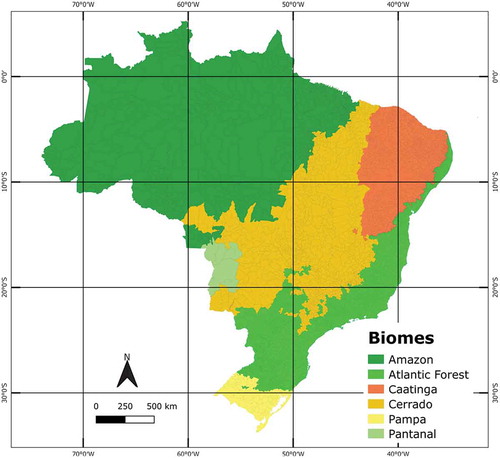
Edaphic conditions ($E$): Dummies related to Brazilian biomes were used as proxy. They are: Amazon Forest ($damz$), Cerrado ($dcer$), Atlantic Forest ($dmatl$), Caatinga ($dcaa$), Pampa ($dpmp$) and Pantanal ($dptn$), the Amazon Forest being the base category. The areas of these biomes can be seen in Figure 1. Two reasons justify this: (i) the soil belonging to the same biome has similar edaphic characteristics, in order to help us explain how appropriate the crops are to a particular type of soil and (ii) to observe the role of biomes in relation to land use.

Figure 1. Brazilian biomes.

Spatial interdependence ($S$): Two spatial dependencies were used in this article and are actually the result of the interaction between the spatial weighting matrix ($W$) and the chosen variables: (i) $WN$, which shows the average of the type $n$ soil in neighbors, serving as an indicator of spatial patterns; and (ii) technological interdependence, in which we have $Wk$ and $Wh$ symbolizing the average use of some technology or technical knowledge in the neighborhood, proxy for a local technological pattern and a possible existence of spillover.

The optimal specification of spatial weight matrices is an area of active research (see Bhattacharjee and Jensen-Butler (2013), Gerkman and Ahlgren (2014), Getis and Aldstadt (2004), Qu and Lee (2015), Seya, Yamagata, and Tsutsumi (2013) and Stakhovych and Bijmolt (2009)). In this study, the choice of spatial weights matrix followed the procedure described in Stakhovych and Bijmolt (2009). The process consists of estimating the proposed spatial model (or that indicated by the Lagrange Multiplier tests) with each candidate matrix, then choosing the spatial weights matrix that yields the smallest value of the Akaike Information Criterion (AIC). Table A1 (in Appendix A) shows the results of the procedure.

3.2.4. Instrumental variables

Within the system of simultaneous equations, land use variables ($N$) can not be treated as exogenous to the model. In order to deal with this endogeneity, in this article, the instrumental variable used is time-lag land use ($N_{\left(t-1\right)}$). This variable can be considered a good instrument because it meets the prerequisites defined by Wooldridge (2015), such as lack of correlation with the error term, and partial correlation with the variable considered endogenous in question, i.e. land use in the current period ($N$). As the model inserts the spatial lag of the land use variables ($WN$) as regressor, this is also an equally endogenous variable and must also be treated. Thus, in this case, the variable in $t-1$ was spatially lagged ($W{N}_{\left(t-1\right)}$) to be used as an instrument. Time-lagged data on the participation of the different types of land use were extracted from the 1995/1996 Agricultural and Livestock Census provided by the IBGE.

In Appendix A (Table A2), the variables are presented in greater detail. Table 1 presents summary statistics for this dataset. Due to the difference between the units of measurement of the variables, we decided to standardize them. In this case, it is useful to obtain regression results for all variables involved – both dependent and independent variables are standardized, for two reasons. First, the unit of measurement of the variables becomes irrelevant, making them equal so that the estimated coefficients (denominated as standard coefficients or beta coefficients) will be given in terms of units of standard deviation, facilitating the interpretation of the results. Second, it is possible to rank the importance of the explanatory variables from the magnitudes of the standardized coefficients, or rather, the larger the standardized coefficient, the ‘more important’ the variable will be compared to the other variables (Wooldridge, 2015). The results should, therefore, be interpreted as the standard deviation. We consider 5,507 Brazilian municipalities as the units of spatial analysis.

Table 1. Summary statistics.

Variable	Mean	Median	Standard deviation	Number of municipalities
Cropland area/(Cropland area + Pasture + Forest)	0.294	0.211	0.265	5507
Pasture area/(Cropland area + Pasture + Forest)	0.467	0.485	0.251	5507
Forest area/(Cropland area + Pasture + Forest)	0.239	0.189	0.190	5507
Mechanization – Number of tractors (with more than 100 hp) by cropland area	0.011	0.003	0.051	5507
Technical assistance – Number of agricultural engineers, agronomists and researchers by cropland area	0.003	0.000	0.121	5507
Average temperature in December, January and February (in °C)	24.602	24.882	1.947	5507
Average temperature in March, April and May (in °C)	22.856	23.370	2.855	5507
Average temperature in June, July and August (in °C)	20.306	20.674	4.121	5507
Average temperature in September, October and November (in °C)	23.160	23.586	3.279	5507
Average precipitation in December, January and February (in mm)	172.163	172.117	74.873	5507
Average precipitation in March, April and May (in mm)	130.146	113.608	63.149	5507
Average precipitation in June, July and August (in mm)	61.091	35.975	56.453	5507
Average precipitation in September, October and November (in mm)	101.032	115.383	51.412	5507

3.3. Exploratory analysis of spatial data: spatial autocorrelation tests

The presence of spatial autocorrelation was tested globally and locally via the Moran and the LISA (Local Indicator of Spatial Association) indexes, respectively. The existence of spatial patterns was verified for the dependent variables (land use) and the technology variables, which will be useful later for observing regional technological patterns and spillovers. Moran’s I coefficients were calculated and their values are reported in Table 2.

Table 2. Spatial autocorrelation statistics – Moran’s I*.

Variable**	Moran’s I	E(I)	p-value***
Cropland (cr)	0.6602	−0.0002	0.001
Pasture (pt)	0.6200	−0.0002	0.001
Forest (ft)	0.5234	−0.0002	0.001
Mechanization – Physical capital (k)	0.2617	−0.0002	0.001
Technical assistance – Human capital (h)	0.5154	−0.0002	0.001

Notes: * The neighborhood matrix $k15$ was chosen using the criterion set forth in Stakhovych and Bijmolt (2009) presented in the appendix (see Table A1). ** The variables are expressed in relation to the total. *** The empirical pseudo-significance is based on 99,999 random permutations.

Given the statistical evidence shown in Table 2, the null hypothesis of spatial randomness below a significance level of 1% is rejected. Coefficient I provides a clear indication that land uses and the variables of technology are autocorrelated in space across the Brazilian municipalities. The magnitude of the statistic informs us that the variables cropland (cr) and pasture (pt) present a strong spatial concentration.

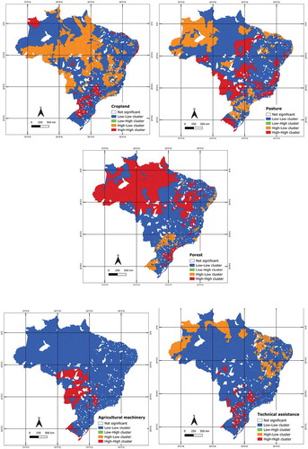
The LISA indicator, proposed by Anselin (1995), has the capacity to capture local patterns of spatial autocorrelation. The local Moran coefficient I ($I_i$) breaks down the global autocorrelation indicator in the local contribution of each observation into four categories: HH – high/high, LL – low/low, HL – high/low, and LH – low/high (Anselin, 2013). The generated cluster maps are shown below. Expectations about the distribution of variables in space were satisfied (Figure 2), demonstrating the reliability of the data used. In addition, we verified that the variables used are not randomly distributed in space, but spatially grouped. This suggests that econometric analysis should incorporate geographic neighborhood effects.

Figure 2. Map of LISA clusters for selected variables.

3.4. Empirical implementation

Land resources are limited, and any decision about their use is interdependent and requires space exclusivity. Thus, if one chooses to plant crops on land, this implies not choosing pasture nor forest, and vice versa. This produces a potential correlation in terms of error (${\epsilon }_j$) of the equations belonging to the system. Therefore, there is a problem of simultaneity of equations that explain land use and the detection of spatial autocorrelation. Note the presence of a cross spatial lag, indicating that the average of the variable of interest in neighbors explains the basic endogenous variable, in addition to the feedback simultaneity, formalizing a concept of circular causation. When using the Spatial Simultaneous Equation System framework, two problems are avoided: (i) a simultaneous estimation method takes into account the correlation between these errors. Methods that estimate each equation alone ignore the correlation between the equations and are therefore not efficient; and (ii) it prevents the omitted variable bias when not excluding the aspect of spatial dependency.

We follow the taxonomy proposed by Rey and Boarnet (2004) for simultaneous spatial equations. To structure the taxonomy, it is useful to note that there are essentially four dimensions to consider: feedback simultaneity, spatial autoregressive lag simultaneity, spatial cross-regressive lag simultaneity and spatial lag in the explanatory variable. Thus, there are four structural models described in Table 3:

Table 3. Model taxonomy.

Model	Equations	Simultaneity	Description
(1)	$N_{j,i}=f\left(N_{-j,i},T_i,C_i,E_i,N_{j\left(t-1\right),i},{\epsilon }_j\right)$	Feedback	In the feedback model, the equation that intends to explain the land use $j$ in region $i$ ($N_{j,i}$) has as determinants the other types of use ($N_{-j,i}$), the use of agricultural technology ($T_i$), climatic conditions ($C_i$), soil conditions ($E_i$) and the land use $j$ in region $i$in the past ($N_{j\left(t-1\right),i}$).
(2)	$N_{j,i}=f\left(W{N}_{j,i},N_{-j,i},T_i,C_i,E_i,N_{j\left(t-1\right),i},{\epsilon }_j\right)$	Feedback and lags	In this model, the equation that aims to explain the use of soil type $j$ in region $i$follows the previous structure with increase of spatial lag in the endogenous variable present on the left side of equation ($W{N}_{j,i}$), where $W$ is the spatial lag matrix.
(3)	$N_{j,i}=f\left(W{N}_{j,i},N_{-j,i},W{N}_{-j,i},T_i,C_i,E_i,N_{j\left(t-1\right),i},{\epsilon }_j\right)$	Feedback, lags and cross-lags	This model has as a novelty the insertion of endogenous variables spatially lagged from the right side ($W{N}_{-j,i}$).
(4)	$N_{j,i}=f\left(W{N}_{j,i},N_{-j,i},W{N}_{-j,i},T_i,W{T}_i,C_i,E_i,N_{j\left(t-1\right),i},{\epsilon }_j\right)$	Feedback, lags, cross-lags and lag in independent variable	Finally, we consider a complete model with feedback, spatial lag, cross-lag and spatial lag in an independent variable, more specifically in the variable of use of agricultural technology ($W{T}_i$).

According to Rey and Boarnet (2004), there are four conditions for identifying an equation in the system, incorporating special dependence:

First condition: The error terms of each equation have zero mean and are not spatially autocorrelated.

Second condition: All endogenous basic variables in the model can be expressed in terms of exogenous variables, additional endogenous variables and error terms¹.

Third condition: The solution of the model for the basic endogenous variables in terms of the exogenous variables and the error terms is unique.

Fourth condition: The number of basic endogenous variables appearing on the right side of an equation must be equal to or less than the number of exogenous variables and additional endogenous variables appearing in the model but not in that equation.

Two procedures will be used to generate the results. The first, proposed by Kelejian and Robinson (1993), resembles the Two-Stage Least Squares (2SLS) method. This estimator can be implemented as follows:

Step 1 (KR1): The values adjusted by the model of each basic endogenous variable appearing on the right side of the equation are obtained by regressing this variable against the exogenous variables ($X$) and their spatial lags ($WX$), where $X=⟨T,C,E⟩$.

Step 2 (KR2): The adjusted values of each additional endogenous variable are obtained, regressing it against the exogenous variables ($X$) and their spatial lags ($WX$) by Ordinary Least Square (OLS).

Step 3 (KR3): The basic and additional endogenous variables in the $ith$ equation are substituted with their adjusted values and the parameters of the equation are then estimated by OLS.

The second procedure, proposed by Kelejian and Prucha (2004), generalizes the estimator considered in Kelejian and Prucha (1998) for a single equation spatially autoregressive model. The proposed Generalized Spatial Two Stage Least Squares (GS2SLS) estimation procedure consists of three steps:

Step 1 (KP1): We estimate the model parameter vector by Two Stage Least Squares (2SLS) using $H_n=⟨N_{\left(t-1\right)},W{N}_{\left(t-1\right)},W^2{N}_{\left(t-1\right)},W^3{N}_{\left(t-1\right)}⟩$ as the instrument matrix. Based on this, we compute the estimates of the residuals.

Step 2 (KP2): We use these estimated values of the residual to estimate the value of its autoregressive parameter (i.e. regressing the residue by its spatial lag), using the generalized method of moments introduced by Kelejian and Prucha (1999).

Step 3 (KP3): This estimate is used to explain the spatial autocorrelation in the residues, using a Cochrane-Orcutt transformation. The model parameters are obtained by estimating the model transformed by 2SLS using $H_n$ as an instrument matrix.

4. Econometric results

Figure 3 presents the determinants of agricultural and forestry land use using a structural model (4), following Kelejian and Robinson (1993) for the estimation procedure. All models estimated can be seen in Appendix B (Tables B1–B4). In this model structure, the coefficients associated with the local use of mechanization ($k$) and technical assistance ($h$) may not be different from zero for any category of land use. Therefore, based on these variables, it is not possible to accept or reject any of the hypotheses.

Table B1. Determinants of agricultural and forest land use for model (1): estimation by System of Simultaneous Equations in Space using procedure of Kelejian and Robinson. Period: 2006.

	Cropland			Pasture			Forest
Explanatory variables	coef.	std. error	t-value	coef.	std. error	t-value	coef.	std. error	t-value
Constant	-0.518	0.027	-19.185	-0.520	0.028	-18.571	-0.441	0.033	-13.364
Mechanization - Physical capital (k)	0.000	0.006	0.000	0.007	0.006	1.167	0.001	0.007	0.143
Technical advice - Human capital (h)	-0.007	0.006	-1.167	0.001	0.006	0.167	-0.008	0.007	-1.143
Climate - December, January and February (cdjf)	0.115	0.042	2.738	-0.055	0.045	-1.222	-0.075	0.052	-1.442
Climate - March, April and May (cmam)	0.029	0.024	1.208	-0.012	0.024	-0.500	-0.007	0.029	-0.241
Climate - June, July and August (cjja)	0.047	0.023	2.043	-0.055	0.025	-2.200	-0.032	0.029	-1.103
Climate - September, October and November (cson)	-0.044	0.040	-1.100	0.053	0.043	1.233	0.124	0.049	2.531
Biome - Caatinga (dcaa)	0.090	0.035	2.571	0.016	0.037	0.432	-0.012	0.044	-0.273
Biome - Cerrado (dcer)	0.102	0.029	3.517	-0.029	0.031	-0.935	-0.054	0.038	-1.421
Biome - Pampa (dpmp)	0.115	0.048	2.396	0.059	0.055	1.073	0.037	0.057	0.649
Biome - Pantanal (dptn)	-0.047	0.150	-0.313	0.099	0.159	0.623	-0.197	0.184	-1.071
Biome - Atlantic Forest (dmatl)	0.134	0.030	4.467	-0.009	0.030	-0.300	-0.039	0.036	-1.083
Cropland (cr)				-0.977	0.026	-37.577	-1.443	0.043	-33.558
Pasture (pt)	-0.906	0.029	-31.241				-1.401	0.042	-33.357
Forest (ft)	-0.672	0.020	-33.600	-0.699	0.029	-24.103
Dependent variable with time lag (Nt-1)	-0.030	0.017	-1.765	-0.026	0.016	-1.625	-0.048	0.014	-3.429
Dependent variable with spatial and time lag (WNt-1)	0.023	0.018	1.278	0.049	0.017	2.882	0.014	0.024	0.583
AIC	5313.14			5904.52			7539.34
R-squared	0.847			0.829			0.771

Table B2. Determinants of agricultural and forest land use for model (2): estimation by System of Simultaneous Equations in Space using procedure of Kelejian and Robinson. Period: 2006.

	Cropland			Pasture			Forest
Explanatory variables	coef.	std. error	t-value	coef.	std. error	t-value	coef.	std. error	t-value
Constant	-0.521	0.027	-19.296	-0.520	0.028	-18.571	-0.437	0.033	-13.242
Dependent variable spatially lagged (prWN)	0.092	0.058	1.586	0.062	0.043	1.442	0.197	0.055	3.582
Mechanization - Physical capital (k)	-0.002	0.006	-0.333	0.008	0.006	1.333	0.001	0.007	0.143
Technical advice - Human capital (h)	-0.011	0.006	-1.833	0.002	0.006	0.333	-0.001	0.007	-0.143
Climate - December, January and February (cdjf)	0.104	0.043	2.419	-0.049	0.045	-1.089	-0.08	0.052	-1.538
Climate - March, April and May (cmam)	0.032	0.025	1.280	-0.019	0.025	-0.760	0.007	0.030	0.233
Climate - June, July and August (cjja)	0.041	0.023	1.783	-0.053	0.025	-2.120	-0.021	0.029	-0.724
Climate - September, October and November (cson)	-0.041	0.040	-1.025	0.046	0.043	1.070	0.113	0.049	2.306
Biome - Caatinga (dcaa)	0.093	0.035	2.657	0.010	0.037	0.270	-0.018	0.044	-0.409
Biome - Cerrado (dcer)	0.104	0.029	3.586	-0.027	0.031	-0.871	-0.059	0.038	-1.553
Biome - Pampa (dpmp)	0.124	0.048	2.583	0.057	0.055	1.036	0.011	0.058	0.190
Biome - Pantanal (dptn)	-0.056	0.150	-0.373	0.118	0.159	0.742	-0.201	0.184	-1.092
Biome - Atlantic Forest (dmatl)	0.139	0.030	4.633	-0.009	0.030	-0.300	-0.040	0.036	-1.111
Cropland (cr)				-0.928	0.043	-21.581	-1.226	0.074	-16.568
Pasture (pt)	-0.840	0.051	-16.471				-1.191	0.072	-16.542
Forest (ft)	-0.618	0.039	-15.846	-0.664	0.037	-17.946
Dependent variable with time lag (Nt-1)	0.002	0.026	0.077	-0.009	0.020	-0.450	-0.009	0.018	-0.500
Dependent variable with spatial and time lag (WNt-1)	-0.023	0.034	-0.676	0.023	0.025	0.920	-0.054	0.031	-1.742
AIC	5312.59			5904.52			7528.56
R-squared	0.847			0.829			0.771

Table B3. Determinants of agricultural and forest land use for model (3): estimation by System of Simultaneous Equations in Space using procedure of Kelejian and Robinson. Period: 2006.

	Cropland			Pasture			Forest
Explanatory variables	coef.	std. error	t-value	coef.	std. error	t-value	coef.	std. error	t-value
Constant	-0.520	0.027	-19.259	-0.519	0.028	-18.536	-0.447	0.033	-13.545
Dependent variable spatially lagged (prWN)	0.548	0.155	3.535	0.687	0.148	4.642	0.737	0.127	5.803
Mechanization - Physical capital (k)	-0.001	0.006	-0.167	0.008	0.006	1.333	0.003	0.007	0.429
Technical advice - Human capital (h)	-0.010	0.006	-1.667	0.001	0.006	0.167	-0.003	0.007	-0.429
Climate - December, January and February (cdjf)	0.094	0.043	2.186	-0.048	0.045	-1.067	-0.073	0.052	-1.404
Climate - March, April and May (cmam)	0.033	0.025	1.320	-0.012	0.025	-0.480	0.002	0.030	0.067
Climate - June, July and August (cjja)	0.045	0.023	1.957	-0.049	0.025	-1.960	-0.015	0.029	-0.517
Climate - September, October and November (cson)	-0.051	0.040	-1.275	0.036	0.043	0.837	0.090	0.049	1.837
Biome - Caatinga (dcaa)	0.087	0.035	2.486	0.002	0.038	0.053	-0.018	0.044	-0.409
Biome - Cerrado (dcer)	0.103	0.029	3.552	-0.022	0.031	-0.710	-0.044	0.038	-1.158
Biome - Pampa (dpmp)	0.123	0.048	2.563	0.038	0.055	0.691	0.026	0.058	0.448
Biome - Pantanal (dptn)	-0.063	0.150	-0.420	0.106	0.159	0.667	-0.205	0.183	-1.120
Biome - Atlantic Forest (dmatl)	0.139	0.030	4.633	-0.011	0.031	-0.355	-0.030	0.036	-0.833
Cropland (cr)				-0.935	0.046	-20.326	-1.339	0.078	-17.167
Pasture (pt)	-0.859	0.051	-16.843				-1.351	0.080	-16.888
Forest (ft)	-0.647	0.049	-13.204	-0.633	0.058	-10.914
Cropland with spatial lag (prWcr)				0.657	0.153	4.294	0.892	0.191	4.670
Pasture with spatial lag (prWpt)	0.436	0.140	3.114				0.908	0.183	4.962
Forest with spatial lag (prWft)	0.349	0.109	3.202	0.426	0.117	3.641
Dependent variable with time lag (Nt-1)	-0.007	0.027	-0.259	-0.008	0.022	-0.364	-0.033	0.019	-1.737
Dependent variable with spatial and time lag (WNt-1)	-0.031	0.034	-0.912	0.009	0.029	0.310	-0.009	0.032	-0.281
AIC	5306.17			5888.51			7506.37
R-squared	0.847			0.831			0.772

Table B4. Determinants of agricultural and forest land use for model (4): estimation by System of Simultaneous Equations in Space using procedure of Kelejian and Robinson. Period: 2006.

	Cropland			Pasture			Forest
Explanatory variables	coef.	std. error	t-value	coef.	std. error	t-value	coef.	std. error	t-value
Constant	-0.526	0.027	-19.481	-0.518	0.028	-18.500	-0.450	0.033	-13.636
Dependent variable spatially lagged (WN)	0.511	0.155	3.297	0.685	0.148	4.628	0.734	0.127	5.780
Mechanization - Physical capital (k)	0.001	0.006	0.167	0.008	0.006	1.333	0.003	0.007	0.429
Technical advice - Human capital (h)	-0.007	0.006	-1.167	0.001	0.006	0.167	-0.003	0.007	-0.429
Physical Capital with spatial lag (Wk)	-0.071	0.023	-3.087	0.022	0.025	0.880	-0.042	0.029	-1.448
Human Capital with spatial lag (Wh)	-0.015	0.026	-0.577	-0.031	0.025	-1.240	0.049	0.028	1.750
Climate - December, January and February (cdjf)	0.093	0.044	2.114	-0.056	0.046	-1.217	-0.063	0.052	-1.212
Climate - March, April and May (cmam)	0.013	0.025	0.520	-0.009	0.025	-0.360	-0.005	0.03	-0.167
Climate - June, July and August (cjja)	0.060	0.024	2.500	-0.053	0.025	-2.120	-0.010	0.029	-0.345
Climate - September, October and November (cson)	-0.065	0.040	-1.625	0.034	0.044	0.773	0.088	0.050	1.760
Biome - Caatinga (dcaa)	0.095	0.035	2.714	0.000	0.038	0.000	-0.014	0.044	-0.318
Biome - Cerrado (dcer)	0.104	0.030	3.467	-0.025	0.031	-0.806	-0.039	0.038	-1.026
Biome - Pampa (dpmp)	0.144	0.049	2.939	0.048	0.056	0.857	0.024	0.058	0.414
Biome - Pantanal (dptn)	-0.056	0.150	-0.373	0.11	0.159	0.692	-0.206	0.183	-1.126
Biome - Atlantic Forest (dmatl)	0.147	0.030	4.900	-0.011	0.031	-0.355	-0.028	0.037	-0.757
Cropland (cr)				-0.923	0.048	-19.229	-1.330	0.082	-16.220
Pasture (pt)	-0.906	0.056	-16.179				-1.338	0.084	-15.929
Forest (ft)	-0.712	0.054	-13.185	-0.621	0.061	-10.180
Cropland with spatial lag (Wcr)				0.653	0.153	4.268	0.887	0.192	4.620
Pasture with spatial lag (Wpt)	0.422	0.140	3.014				0.901	0.185	4.870
Forest with spatial lag (Wft)	0.378	0.109	3.468	0.423	0.117	3.615
Dependent variable with time lag (Nt-1)	-0.035	0.029	-1.207	-0.003	0.023	-0.130	-0.031	0.019	-1.632
Dependent variable with spatial and time lag (WNt-1)	-0.030	0.035	-0.857	0.012	0.030	0.400	-0.004	0.032	-0.125
AIC	5296.38			5890.88			7506.74
R-squared	0.847			0.830			0.772
Breusch-Pagan test of independence	735.54***

Figure 3. Determinants of agricultural and forest land use for model (4): estimation by system of simultaneous equations in space using procedure of Kelejian and Robinson (1993) – Period: 2006.

In turn, the coefficient associated with spatially lagged physical capital variable ($Wk$) is negative for cropland use (Figure 3(a)). In this case, if $Wk$ increases by one standard deviation, on average, the cropland area reduces by 0.071 standard deviation. This result follows the validation line of the Borlaug hypothesis, that is, the use of agricultural technology in the form of physical capital (agricultural machinery) maintains/reduces agricultural areas, thus preserving forest areas. Note that this effect can only be perceived when we take into account the use of technology in a region (via the application of spatial lag), rather than a municipality alone. Another result to be highlighted is the effect of the spatially lagged agricultural human capital variable ($Wh$) on forest areas (Figure 3(c)). We found the positive effect of 0.049 standard deviation of forest area for each standard deviation of $Wh$. Thus, it is possible to affirm that the regional presence of qualified people assists in the preservation of green areas. Again, we have a result that meets the Borlaug hypothesis. We believe that two points justify the fact that only spatially lagged variables are significant. First, there may be some type of loan or rent of agricultural machinery between rural producers, and, secondly, skilled workers can move across small distances, thus serving more than one rural property.

Both results also validate hypothesis 3, that of the existence of technological-agricultural spillover among the regions. Some channels may explain this technology spillover. The best known is explained by epidemiological models (see Griliches, 1957; Mansfield, 1961) which report the existence of a contagious effect or ‘word-of-mouth’ communication. By realizing the gains of their neighbors (e.g. productivity increase), economic agents, in this case farmers, seek to adopt a similar technology in order to enjoy the same benefits. It should be noted that this contagion effect occurs between agents from the same region and across regions (e.g. municipalities), the latter being explained by the variables $Wk$ and $Wh$. The economic literature identifies two other basic approaches to technological diffusion, namely, the models of balanced diffusion (David, 1969; Davies, 1979; Stoneman & Ireland, 1983) and evolutionary models (Iwai, 1984a, 1984b; Metcalfe, 2002; Nelson & Winter, 2002; Silverberg, Dosi, & Orsenigo, 1988).

Figure 3 also shows that the different land uses are spatially dependent (variable WN). This indicates a spatial correlation of land use; therefore, municipalities with the presence of cropland are surrounded by municipalities that also have a significant presence of cropland, regions with the presence of pasture are surrounded by pasture and forest areas are surrounded by forests.

Figure 3 also presents aspects related to interdependence and competition among land uses. Note that cropland use undergoes greater competition from pasture use (Figure 3(a)), with an increase of one standard deviation of pasture reducing cropland area by 0.906 standard deviation, on average, whereas the forestry effect was of −0.712 standard deviation. The opposite is also true. That is, pasture use undergoes greater cropland competition (the increase of one standard deviation of cropland area reduces 0.923 standard deviation of pasture – see Figure 3(b)). This dispute effect increases when we observe the ratio between agricultural uses (cropland and pasture) versus forestry (Figure 3(c)). We found that for each increase of one standard deviation of cropland, there is a reduction of 1.330 standard deviation of forestry, an effect that is slightly lower than the pasture-forestry ratio (−1.338 standard deviation). This indicates that there is no harmonious relationship between land uses for agricultural and forestry purposes. This aspect can be mitigated by the use of technology. As we are working with a beta coefficient, the magnitude of the coefficients found reveals the importance of the variable. It can be seen that in all the equations the variables that represent the other land uses presented the greatest magnitudes, revealing the importance of a modeling in the form of simultaneous equations. It is also worth noting that the Breusch-Pagan test rejects the hypothesis that the errors in the two estimated equations are not correlated. This provides empirical evidence that producers’ decisions about how to allocate land for different types of use should be interdependent, and that in this case the use of simultaneous estimation methods such as the one proposed here is more efficient than the estimation of each system equation in isolation.

The results related to the climatic conditions variables inform us that the cropland areas expand when the temperature and/or precipitation increase in the periods of December/January/February ($djf$) and June/July/August ($jja$). Pasture areas reduce when the temperature and/or precipitation increase significantly in the months of June/July/August (jja). Finally, forest areas increase when the temperature and/or precipitation rise during the months of September/October/November ($son$).

The biome dummies, which play the role of control of soil conditions, are mostly different from zero in the cropland equation. Through them, it can be observed that there is a higher incidence of cropland in the Atlantic Forest areas, followed by the Pampa, Cerrado, Caatinga and Amazon Forest.

Figure 4 reinforces the results already discussed here, using the estimation procedure proposed by Kelejian and Prucha (2004). All other models estimated using the procedure of Kelejian and Prucha (2004) can be seen in Appendix B (Tables B5–B8). We emphasize the negative sign between the spatially lagged physical capital variable (which indicates a regional technology pattern) and the cropland and pasture uses. In this case, if $Wk$ increases by one standard deviation, on average, cropland and pasture areas fall by 0.02 standard deviation (see Figure 4(a,b)). Again, this result corroborates the Borlaug hypothesis.

Table B5. Determinants of agricultural and forest land use for model (1): estimation by System of Simultaneous Equations in Space using procedure of Kelejian and Prucha. Period: 2006.

	Cropland			Pasture			Forest
Explanatory variables	coef.	std. error	t-value	coef.	std. error	t-value	coef.	std. error	t-value
Constant	-0.004	0.012	-0.333	-0.004	0.013	-0.308	-0.004	0.017	-0.235
Mechanization - Physical capital (k)	0.000	0.003	0.000	0.001	0.003	0.333	0.001	0.004	0.250
Technical advice - Human capital (h)	0.001	0.003	0.333	0.001	0.003	0.333	0.001	0.004	0.250
Climate - December, January and February (cdjf)	0.001	0.019	0.053	0.001	0.020	0.050	0.001	0.027	0.037
Climate - March, April and May (cmam)	-0.013	0.011	-1.182	-0.014	0.012	-1.167	-0.017	0.015	-1.133
Climate - June, July and August (cjja)	-0.015	0.010	-1.500	-0.016	0.011	-1.455	-0.021	0.014	-1.500
Climate - September, October and November (cson)	0.040	0.019	2.105	0.042	0.020	2.100	0.056	0.026	2.154
Biome - Caatinga (dcaa)	0.024	0.017	1.412	0.025	0.017	1.471	0.033	0.023	1.435
Biome - Cerrado (dcer)	-0.003	0.013	-0.231	-0.003	0.014	-0.214	-0.005	0.018	-0.278
Biome - Pampa (dpmp)	0.024	0.022	1.091	0.025	0.023	1.087	0.031	0.030	1.033
Biome - Pantanal (dptn)	0.020	0.072	0.278	0.022	0.076	0.289	0.028	0.099	0.283
Biome - Atlantic Forest (dmatl)	-0.002	0.014	-0.143	-0.003	0.014	-0.214	-0.004	0.019	-0.211
Cropland (cr)				-1.056	0.002	-528.000	-1.374	0.004	-343.500
Pasture (pt)	-0.947	0.002	-473.500				-1.301	0.004	-325.250
Forest (ft)	-0.726	0.002	-363.000	-0.767	0.002	-383.500
R-squared	0.963			0.959			0.931

Table B6. Determinants of agricultural and forest land use for model (2): estimation by System of Simultaneous Equations in Space using procedure of Kelejian and Prucha. Period: 2006.

	Cropland			Pasture			Forest
Explanatory variables	coef.	std. error	t-value	coef.	std. error	t-value	coef.	std. error	t-value
Constant	-0.004	0.012	-0.333	-0.004	0.013	-0.308	-0.006	0.016	-0.375
Dependent variable spatially lagged (WN)	0.001	0.002	0.500	0.002	0.002	1.000	0.005	0.003	1.667
Mechanization - Physical capital (k)	0.000	0.003	0.000	0.001	0.003	0.333	0.001	0.004	0.250
Technical advice - Human capital (h)	0.000	0.003	0.000	0.001	0.003	0.333	0.001	0.004	0.250
Climate - December, January and February (cdjf)	0.001	0.019	0.053	0.001	0.020	0.050	0.000	0.026	0.000
Climate - March, April and May (cmam)	-0.013	0.011	-1.182	-0.014	0.011	-1.273	-0.018	0.015	-1.200
Climate - June, July and August (cjja)	-0.014	0.010	-1.400	-0.015	0.011	-1.364	-0.020	0.014	-1.429
Climate - September, October and November (cson)	0.039	0.018	2.167	0.041	0.019	2.158	0.054	0.025	2.160
Climate - December, January and February squared (cdjf2)	-0.019	0.015	-1.267	-0.020	0.016	-1.250	-0.025	0.021	-1.190
Climate - March, April and May squared (cmam2)	0.029	0.011	2.636	0.030	0.012	2.500	0.039	0.015	2.600
Climate - June, July and August squared (cjja2)	0.004	0.007	0.571	0.004	0.007	0.571	0.005	0.009	0.556
Climate - September, October and November squared (cson2)	-0.022	0.014	-1.571	-0.023	0.015	-1.533	-0.030	0.019	-1.579
Biome - Caatinga (dcaa)	0.024	0.016	1.500	0.025	0.017	1.471	0.033	0.022	1.500
Biome - Cerrado (dcer)	-0.002	0.013	-0.154	-0.003	0.014	-0.214	-0.003	0.018	-0.167
Biome - Pampa (dpmp)	0.025	0.022	1.136	0.027	0.023	1.174	0.034	0.030	1.133
Biome - Pantanal (dptn)	0.021	0.071	0.296	0.022	0.075	0.293	0.030	0.098	0.306
Biome - Atlantic Forest (dmatl)	-0.001	0.013	-0.077	-0.002	0.014	-0.143	-0.002	0.018	-0.111
Cropland (cr)				-1.053	0.003	-351.000	-1.372	0.005	-274.400
Pasture (pt)	-0.947	0.003	-315.667				-1.300	0.005	-260.000
Forest (ft)	-0.724	0.002	-362.000	-0.764	0.003	-254.667
R-squared	0.964			0.959			0.931

Table B7. Determinants of agricultural and forest land use for model (3): estimation by System of Simultaneous Equations in Space using procedure of Kelejian and Prucha. Period: 2006.

	Cropland			Pasture			Forest
Explanatory variables	coef.	std. error	t-value	coef.	std. error	t-value	coef.	std. error	t-value
Constant	-0.007	0.012	-0.583	-0.007	0.013	-0.538	-0.009	0.017	-0.529
Dependent variable spatially lagged (WN)	0.217	0.047	4.617	0.221	0.047	4.702	0.225	0.047	4.787
Mechanization - Physical capital (k)	0.001	0.003	0.333	0.001	0.003	0.333	0.001	0.004	0.250
Technical advice - Human capital (h)	0.001	0.003	0.333	0.001	0.003	0.333	0.001	0.004	0.250
Climate - December, January and February (cdjf)	0.002	0.02	0.100	0.002	0.021	0.095	0.002	0.027	0.074
Climate - March, April and May (cmam)	-0.011	0.011	-1.000	-0.012	0.011	-1.091	-0.015	0.015	-1.000
Climate - June, July and August (cjja)	-0.01	0.011	-0.909	-0.011	0.011	-1.000	-0.015	0.015	-1.000
Climate - September, October and November (cson)	0.031	0.019	1.632	0.033	0.02	1.650	0.043	0.026	1.654
Biome - Caatinga (dcaa)	0.024	0.016	1.500	0.025	0.017	1.471	0.032	0.022	1.455
Biome - Cerrado (dcer)	0.002	0.013	0.154	0.002	0.014	0.143	0.003	0.018	0.167
Biome - Pampa (dpmp)	0.024	0.022	1.091	0.026	0.023	1.130	0.033	0.03	1.100
Biome - Pantanal (dptn)	0.02	0.071	0.282	0.021	0.075	0.280	0.028	0.098	0.286
Biome - Atlantic Forest (dmatl)	0.003	0.014	0.214	0.003	0.014	0.214	0.003	0.019	0.158
Cropland (cr)				-1.051	0.004	-262.750	-1.367	0.006	-227.833
Pasture (pt)	-0.948	0.003	-316.000				-1.299	0.005	-259.800
Forest (ft)	-0.727	0.003	-242.333	-0.765	0.003	-255.000
Cropland with spatial lag (Wcr)				0.227	0.05	4.540	0.293	0.065	4.508
Pasture with spatial lag (Wpt)	0.208	0.045	4.622				0.284	0.061	4.656
Forest with spatial lag (Wft)	0.161	0.034	4.735	0.17	0.036	4.722
R-squared	0.964			0.959			0.932

Table B8. Determinants of agricultural and forest land use for model (4): estimation by System of Simultaneous Equations in Space using procedure of Kelejian and Prucha. Period: 2006.

	Cropland			Pasture			Forest
Explanatory variables	coef.	std. error	t-value	coef.	std. error	t-value	coef.	std. error	t-value
Constant	-0.010	0.012	-0.833	-0.010	0.013	-0.769	-0.013	0.017	-0.765
Dependent variable spatially lagged (WN)	0.213	0.047	4.532	0.218	0.047	4.638	0.223	0.047	4.745
Mechanization - Physical capital (k)	0.001	0.003	0.333	0.001	0.003	0.333	0.001	0.004	0.250
Technical advice - Human capital (h)	0.001	0.003	0.333	0.001	0.003	0.333	0.001	0.004	0.250
Physical Capital with spatial lag (Wk)	-0.020	0.011	-1.818	-0.020	0.011	-1.818	-0.027	0.015	-1.800
Human Capital with spatial lag (Wh)	0.002	0.011	0.182	0.002	0.011	0.182	0.002	0.015	0.133
Climate - December, January and February (cdjf)	0.004	0.020	0.200	0.004	0.021	0.190	0.005	0.027	0.185
Climate - March, April and May (cmam)	-0.014	0.011	-1.273	-0.015	0.012	-1.250	-0.020	0.015	-1.333
Climate - June, July and August (cjja)	-0.008	0.011	-0.727	-0.008	0.011	-0.727	-0.011	0.015	-0.733
Climate - September, October and November (cson)	0.027	0.019	1.421	0.028	0.020	1.400	0.037	0.026	1.423
Biome - Caatinga (dcaa)	0.027	0.016	1.688	0.028	0.017	1.647	0.037	0.023	1.609
Biome - Cerrado (dcer)	0.005	0.013	0.385	0.005	0.014	0.357	0.006	0.018	0.333
Biome - Pampa (dpmp)	0.028	0.022	1.273	0.030	0.023	1.304	0.038	0.030	1.267
Biome - Pantanal (dptn)	0.022	0.071	0.310	0.023	0.075	0.307	0.031	0.098	0.316
Biome - Atlantic Forest (dmatl)	0.006	0.014	0.429	0.006	0.015	0.400	0.008	0.019	0.421
Cropland (cr)				-1.051	0.004	-262.750	-1.367	0.006	-227.833
Pasture (pt)	-0.948	0.003	-316.000				-1.298	0.005	-259.600
Forest (ft)	-0.727	0.003	-242.333	-0.766	0.003	-255.333
Cropland with spatial lag (Wcr)				0.223	0.050	4.460	0.288	0.065	4.431
Pasture with spatial lag (Wpt)	0.205	0.045	4.556				0.279	0.061	4.574
Forest with spatial lag (Wft)	0.160	0.034	4.706	0.169	0.036	4.694
R-squared	0.963			0.959			0.932

Figure 4. Determinants of agricultural and forest land use for model (4): estimation by system of simultaneous equations in space using procedure of Kelejian and Prucha (2004) – Period: 2006.

It was also possible to observe the competitive relationship between land uses. The way in which the uses of agriculture and pasture exert great pressure on forests can be clearly seen. With each standard deviation of increase in areas of cropland and pasture, 1.367 and 1.298 standard deviation of forest areas are reduced respectively (see Figure 4(c)). In the supplementary material, we show which regions are most likely to replace forestry by cropland or pasture.

In addition, another specification was used as a robustness test. Following Huang, Bruemmer, and Huntsinger (2017) and Ma, Feng, Reidsma, Qu, and Heerink (2014), we estimate the coefficients using the function in its Translog format. Unlike the traditional Cobb-Douglas and CES (Mal, Manjunatha, Bauer, & Ahmed, 2011; Manjunatha, Anik, Speelman, & Nuppenau, 2013), the Translog function imposes no restriction on the values of the elasticity of substitution, nor does it assume homogeneity of the function (Wilson, Hadley, Ramsden, & Kaltsas, 1998). Thus, it is convenient to use the Translog function in the measurement of non-neutral technological modifications². The results reinforce what has been described so far, that is, we find again (1) a negative relationship between the physical capital variable (mechanization) with spatial lag and land use for agriculture, and a positive relationship between the spatially lagged agricultural human capital variable (technical assistance) over forest areas; (2) the existence of technology spillover; and (3) the competitive relationship between land uses for agricultural and forestry purposes that can be mitigated with the use of these technologies.

5. Discussion

From the mid-1960s, Brazilian agriculture began its modernization process following the so-called Green Revolution. Analyzing indicators of modernization in agriculture, such as the number of tractors used in agricultural establishments, there has been a significant transformation in the Brazilian agriculture. According to the Agricultural Census, there were about 8,372 tractors in use in Brazil in 1950, 665,280 in 1985 and 1,228,634 in 2017. In turn, the best land-use practices are directly related to the number of skilled people working in rural areas. The number of agricultural engineers, agronomists, zootechnicians and researchers in agronomical sciences and zootechnics went from 17,779 in 2005 to 23,972 in 2017. Despite the advances in the incorporation of innovations by agriculture, many rural producers in Brazil, owning mostly small establishments, still have difficulties to access and use modern production processes and methods, such as tractors, fertilizers, soil correctives, pesticides, storage units, as well as financing, technical guidance, cooperativism, among other resources (Gasques, Vieira Filho, & Navarro, 2010). From a total of 5.2 million rural establishments in Brazil, identified in the IBGE’s 2006 Census of Agriculture, only 983,000 used high technology. Although technological innovation processes in agriculture have enabled great advances, it is important to recognize that there is a highly technological and dynamic agriculture in Brazil, alongside another which is still very poor and in the margins of the market.

The ‘Brazilian success’ in terms of agricultural production and productivity was accompanied by worsening socioeconomic inequality in rural areas (Amann & Baer, 2006; Da Silva, 1996; Franko, 2007; Martinelli, Naylor, Vitousek, & Moutinho, 2010; Ocampo, 2009). Family farming is represented by 4.4 million agricultural establishments in the country (84.4% of the total), but covers only 80 million ha (24.3% of the total area). The average area of family farms was 18.3 ha, while that of non-family farms was 330 ha (IBGE, 2011). In addition, 3.9 million establishments (39% of the total) were administered by illiterate people or could read and write without attending school and in 43% of cases had not completed elementary school. This fact deepens inequality in rural areas as technical improvement and consequent increase in productivity correlate with the education level of the producer (IBGE, 2011). In turn, the high concentration of income of Brazilian rural households reflects the scenario of poor land distribution, low education and little access to more efficient forms of production. In 2010, according to data from the Institute of Applied Economic Research (Ipea), the Gini coefficient (a measure of inequality, with values close to 1 representing greater inequality) in the Brazilian countryside was 0.727. Coefficients above 0.6 represent extremely high levels of social inequality.

Environmental degradation is another consequence of the growth of Brazilian agriculture (Niewöhner et al., 2016). The Atlantic Forest, Cerrado (tropical savanna) and Amazon Forest biome are the most affected (Carvalho, de Marco, & Ferreira Junior, 2009; Nepstad et al., 2009; Phillips et al., 2009; Ribeiro, Metzger, Martensen, Ponzoni, & Hirota, 2009; Scouvart et al., 2008; de Las Heras, Lake, Lovett, & Peres, 2012; Ferreira, Ferreira, Miziara, & Soares-Filho, 2013; Ferreira et al., 2014; Bell, Caviglia-Harris, & Cak, 2015; Lewis, Edwards, & Galbraith, 2015; Sloan & Sayer, 2015; Barlow et al., 2016, 2018). Originally, the Atlantic Forest biome occupied more than 1.3 million km², but due to human activities in particular agriculture and urbanization today remains about 10% of its original coverage. Ribeiro et al. (2009) show that more than 80% of the remaining fragments are smaller than 50 ha (most of them located in coastal areas) and nature reserve areas protect only 10% of the remaining forest. In turn, the Cerrado (tropical savanna) is the second most important agricultural biome in Brazil covering about 2 million km². Estimates show that half of the Cerrado has already been replaced by agricultural land or pasture (Carvalho et al., 2009; Ferreira et al., 2013; Garcia & Ballester, 2016). In addition, about 20% of native and endemic species no longer occur in protected areas and at least 137 species of animals that occur in the Cerrado are threatened with extinction (Colli, Bastos, & Araújo, 2002; Klink & Machado, 2005). In the Brazilian Amazon, deforestation is driven by livestock, wood extraction and road opening in the region (Bell et al., 2015; de Las Heras et al., 2012; Scouvart et al., 2008). Despite its large extension (4.1 million km²), the Amazonian ecosystem is fragile. The forest lives on its own organic material in a humid environment with abundant rainfall. The slightest interference can cause irreversible damage to your delicate balance. Some studies indicate that about 20% of its original area was degraded by human action (Barlow et al., 2018, 2016; Bell et al., 2015; de Las Heras et al., 2012; Lewis et al., 2015; Phillips et al., 2009; Scouvart et al., 2008).

In section 4 we observed that the use of technological capital (mechanization and technical assistance) combined with good land-use practices can lead to productivity increases without the need to change large ranges of natural cover. If the mechanization of a region ($Wk$) increases by a standard deviation, on average, crop areas will be reduced by 0.071 standard deviation (see Figure 3(a)). This result follows the validation line of the Borlaug hypothesis, that is, the use of agricultural technology in the form of physical capital (agricultural machinery) maintains/reduces agricultural areas, thus preserving forest areas. In addition, we found the positive effect of 0.049 standard deviation of forest areas for each standard deviation of technical assistance in a neighborhood ($Wh$) (see Figure 3(c)). If this is true, there is much to be done in terms of better land use in Brazil, since a large portion of farmers/ranchers have no contact with modern equipment and practices.

Brazilian small farmers need, more than ever, access to information, knowledge and technological innovations. And the institutions of development, research and extension must act intelligently and concertedly to develop solutions that enable the increase in performance and the economic insertion of small farmers, respecting the regional and cultural diversities of the country. Supportive public policies, appropriate technologies, credit and training are among the critical points for these less favored segments to access and use agricultural innovations.

The results found in this article warn us that agricultural technology, whether in the form of equipment or more qualified personnel, should not be seen as a villain in the process of environmental preservation. On the contrary, technology should ensure food safety in perfect harmony with environmental conservation. It is up to governmental bodies to create incentives suitable for the good use of these technologies, aiming to increase the productivity of each area used, thus enabling a more sustainable agriculture.

6. Conclusion

This article attempted to understand the relationship between the adoption of technology (mechanization and technical assistance) and agricultural and forestry land use in Brazilian municipalities. The questions that guided this study were: (i) what is the impact of technological elements on the use of agricultural and forestry land in Brazil? And (ii) is there any influence of the neighborhood in this relationship? To answer these, the variables of agricultural and forestry land use were regressed in relation to mechanization and technical assistance variables. In addition, other factors were considered in the equations, such as climate, soil conditions and spatial interdependence.

Three points stand out in this article. First, most of the results showed some relationship between the variables of agricultural capital (mechanization and technical assistance) and land use for cropland, pasture and forestry. Our approach highlights the importance of the regional technological pattern (represented by spatially lagged technological variables) on land use. Here, the results corroborate the Borlaug hypothesis, which holds that the use of agricultural technologies can enable the maintenance of agricultural areas while preserving forest areas. In addition, with the incorporation of spatially lagged technological variables, we could observe the presence of technology spillovers in agriculture, validating hypothesis 3. Second, we found evidence of competition between land uses. The dispute is more intense when we observe the relationship between agricultural uses (cropland and pasture) versus forestry. Observing the results of the complete models, it is possible to affirm that, on average, each standard deviation of increase in areas for cropland and pasture respectively reduces 1.33 and 1.23 standard deviation of forest area. We believe that the use of technology can mitigate this competition relationship. The forest areas that suffer the greatest pressure are located in the Atlantic Forest biome. Third, from a methodological point of view, this article innovates by making use of the Simultaneous Equations System approach for space. The main model considered feedback effects, lags, cross-lags and lag in the independent variable. In addition, we considered two estimation procedures: Kelejian and Robinson (1993) and Kelejian and Prucha (2004).

This article contributes to the empirical literature on the impacts of agricultural technology, in particular mechanization and technical assistance on agricultural and forestry land use in Brazil, opening a new debate on this research topic. Future work may look at land use impacts from other types of technology such as the use of irrigation pivots and the adoption of the crop-pasture-forest system. In addition, this study serves to motivate future work that may advance this theme, investigating the impacts of technology on biome areas.

Acknowledgments

Ademir Rocha acknowledges financial support from Rede Clima (CNPq Grant 380931/2018-4). Eduardo Gonçalves and Eduardo Almeida acknowledges financial support from National Council for Scientific and Technological Development (CNPq), the Brazilian Federal Agency for Support and Evaluation of Graduate Education (CAPES) and the Minas Gerais State Research Foundation (FAPEMIG).

Disclosure statement

No potential conflict of interest was reported by the authors.

Supplementary material

Supplemental data for this article can be accessed here.

Additional information

Funding

This work was supported by the Conselho Nacional de Desenvolvimento Científico e Tecnológico [306057/2015-8];Fundação de Amparo à Pesquisa do Estado de Minas Gerais [APQ-03151-16];Coordination for the Improvement of Higher Education Personnel – CAPES [001].

Notes

1. It is worth noting here the difference between basic and additional endogenous variables. The first are those that appear on the left side of the equations, while the latter are those that appear on the right side of the equations and are functions of the basic endogenous variables (Rey & Boarnet, 2004).

2. The econometric implementation of the main model as well as the robustness models occurred in the R environment using essentially the ‘spdep’ (Bivand et al., 2011), ‘systemfit’ (Henningsen and Hamann, 2007), ‘bbmle’ (Bolker, 2017) and ‘micEcon’ (Henningsen & Toomet, 2010) packages.

Appendices

Appendix A. Auxiliary tables.

Table A1. Stakhovych and Bijmolt Criteria for selection of spatial lag matrix*.

Spatial lag matrix	Cropland (cr)	Pasture (pt)	Forest (ft)
1-nearest neighbor (k1)	7635.49	7815.27	9378.89
5-nearest neighbors (k5)	7288.16	7724.41	9337.82
10-nearest neighbors (k10)	7183.67	7715.99	9357.30
15-nearest neighbors (k15)	7125.28	7670.22	9319.87
20-nearest neighbors (k20)	7138.73	7684.61	9339.26

Note: *The values within the table represent the Akaike criterion (AIC). The 15-nearest neighbors (k15) matrix was selected.

Table A2. Description of the variables.

	Description		Source	Period
I. Endogenous Variables (N) Land Use
cr	Cropland area / (Cropland area + Pasture + Forest)		Agricultural Census (IBGE)	2006
pt	Pasture area / (Cropland area + Pasture + Forest)
ft	Forest area / (Cropland area + Pasture + Forest)
II. Exogenous Variables (T) Agricultural Technology
k	Mechanization - Number of tractors (with more than 100 hp) by cropland area		Agricultural Census (IBGE)	2006
h	Technical asssistance - Number of agricultural engineers, agronomists and researchers by cropland area		RAIS	2006
(C) Climatic Conditions
tdjf	Average temperature in December, January and February (in °C)		NCEP-DOE Reanalysis 2 project and Climate Hazards group Infrared Precipitation with Station (CHIRPS)	2005-2006
tmam	Average temperature in March, April and May (in °C)
tjja	Average temperature in June, July and August (in °C)
tson	Average temperature in September, October and November (in °C)
pdjf	Average precipitation in December, January and February (in mm)
pmam	Average precipitation in March, April and May (in mm)
pjja	Average precipitation in June, July and August (in mm)
pson	Average precipitation in September, October and November (in mm)
cdjf	Interaction between variables tdjf and pdjf		Self elaboration	2005-2006
cmam	Interaction between variables tmam and pmam
cjja	Interaction between variables tjja and pjja
cson	Interaction between variables tson and pson
(E) Edaphic Conditions
damz	Biome - Amazon (= 1)		IBGE (shapefile)	2006
dcer	Biome - Cerrado (= 1)
dmatl	Biome - Atlantic Forest (= 1)
dcaa	Biome - Caatinga (= 1)
dpmp	Biome - Pampa (= 1)
dptn	Biome - Pantanal (= 1)
(S) Spatial Interdependence
Wk, Wh		Technological spillover - average number of tractors and qualified professionals in the nearest neighbors	Self elaboration	2006
WN		Spatial dependence - average of the type n soil used in the nearest neighbors
III. Variable Instruments (time-lag land use)
cr(t-1)	Cropland area / (Cropland area + Pasture + Forest) with time lag		Agricultural Census (IBGE)	1995/1996
pt(t-1)	Pasture area / (Cropland area + Pasture + Forest) with time lag
ft(t-1)	Forest area / (Cropland area + Pasture + Forest) with time lag

Appendix B. Results.

References

- Adams, R.M. (1989). Global climate change and agriculture: An economic perspective. American Journal of Agricultural Economics, 71(5), 1272–1279.
- Aguiar, A.P.D., Câmara, G., & Escada, M.I.S. (2007). Spatial statistical analysis of land-use determinants in the Brazilian Amazonia: Exploring intra-regional heterogeneity. Ecological Modelling, 209(2), 169–188.
- Amann, E., & Baer, W. (2006). Economic orthodoxy versus social development? The dilemmas facing Brazil’s labour government. Oxford Development Studies, 34, 219–241.
- Angelsen, A., & Kaimowitz, D. (1999). Rethinking the causes of deforestation: Lessons from economic models. The World Bank Research Observer, 14(1), 73–98.
- Angus, A., Burgess, P.J., Morris, J., & Lingard, J. (2009). Agriculture and land use: Demand for and supply of agricultural commodities, characteristics of the farming and food industries, and implications for land use in the UK. Land Use Policy, 26, 230–242.
- Anselin, L. (1995). Local indicators of spatial association - LISA. Geographical Analysis, 27(2), 93–115.
- Anselin, L. (2013). Spatial econometrics: Methods and models. London: Springer Science & Business Media.
- Arima, E.Y., Richards, P., Walker, R., & Caldas, M.M. (2011). Statistical confirmation of indirect land use change in the Brazilian Amazon. Environmental Research Letters, 6(2), 024010.
- Bandiera, O., & Rasul, I. (2006). Social networks and technology adoption in Northern Mozambique. The Economic Journal, 116(514), 869–902.
- Barlow, J., França, F., Gardner, T.A., Hicks, C.C., Lennox, G.D., Berenguer, E., … Graham, N.A.J. (2018). The future of hyperdiverse tropical ecosystems. Nature, 559(7715), 517.
- Barlow, J., Lennox, G.D., Ferreira, J., Berenguer, E., Lees, A.C., Nally, R.M., & Gardner, T.A. (2016). Anthropogenic disturbance in tropical forests can double biodiversity loss from deforestation. Nature, 535(7610), 144.
- Barros, G. (2009). Brazil: The challenges in becoming an agricultural superpower. In L. Brainard & L. Martinez-Diaz (Eds.), Brazil as an economic superpower? Understanding Brazil’s changing role in the global economy (pp. 2–35). Washington, DC: Brookings Institution Press.
- Bell, A.R., Caviglia-Harris, J.L., & Cak, A.D. (2015). Characterizing land-use change over space and time: Applying principal components analysis in the Brazilian Legal Amazon. Journal of Land Use Science, 10(1), 19–37.
- Best, J., McKemey, K., & Underwood, M. (1998). CARE Bangladesh INTERFISH Project: Output of Purpose Review. Reading: University of Reading.
- Bhattacharjee, A., & Jensen-Butler, C. (2013). Estimation of the spatial weights matrix under structural constraints. Regional Science and Urban Economics, 43(4), 617–634.
- Bivand, R., Anselin, L., Berke, O., Bernat, A., Carvalho, M., Chun, Y., ... & Lewin-Koh, N. (2011). spdep: Spatial dependence: Weighting schemes, statistics and models. Retrieved from http://CRAN.R-project.org/package=spdep
- Bolker, B. (2017). Maximum likelihood estimation and analysis with the bbmle package. Retrieved from https://cran.r-project.org/web/packages/bbmle/bbmle.pdf
- Carvalho, F.M.V., de Marco, P., & Ferreira Junior, L.G. (2009). The Cerrado in to pieces: Habitat fragmentation as a function of landscape use in the savannas of central Brazil. Biological Conservation, 142, 1392–1403.
- Case, A. (1992). Neighborhood influence and technological change. Regional Science and Urban Economics, 22(3), 491–508.
- Chakir, R., & Le Gallo, J. (2013). Predicting land use allocation in France: A spatial panel data analysis. Ecological Economics, 92, 114–125.
- Colli, G.R., Bastos, R.P., & Araújo, A.B. (2002). The character and dynamics of the Cerrado herpetofauna. In P.S. Oliveira & R.J. Marquis (Eds.), The cerrrados of Brazil: Ecology and natural history of a neotropical savanna (pp. 223–241). New York, NY: Columbia University Press.
- Conley, T.G., & Udry, C.R. (2010). Learning about a new technology: Pineapple in Ghana. The American Economic Review, 100(1), 35–69.
- Da Silva, J.G. (1996). A nova dinâmica da agricultura brasileira. Campinas: Instituto de Economia - UNICAMP.
- David, P.A. (1969). A Contribution to the Theory of Diffusion. Stanford: Research Center in Economic Growth Stanford University.
- Davies, S. (1979). The diffusion of process innovations. Cambridge: Cambridge University Press Archive.
- de Las Heras, A., Lake, I.R., Lovett, A., & Peres, C. (2012). Future deforestation drivers in an Amazonian ranching frontier. Journal of Land Use Science, 7(4), 365–393.
- Decker, W.L., Jones, V.K., & Achutuni, R. (1986). The impact of climate change from increased atmospheric carbon dioxide on american agriculture. Washington: US Department of Energy.
- Ervin, C.A., & Ervin, D.E. (1982). Factors affecting the use of soil conservation practices: Hypotheses, evidence, and policy implications. Land Economics, 58(3), 277–292.
- Evenson, R.E., & Alves, D.C.O. (2009). Technology, climate change, productivity and land use in Brazilian agriculture. Planejamento E Políticas Públicas, 18(1), 223–260.
- Faria, W.R., & Haddad, E.A. (2017). Modeling land use and the effects of climate change in Brazil. Climate Change Economics, 8(1), 1750002.
- Ferreira, J., Aragao, L.E.O.C., Barlow, J., Barreto, P., Berenguer, E., Bustamante, M., … Zuanon, J. (2014). Environment and Development. Brazil’s environmental leadership at risk. Science, 346, 706–707.
- Ferreira, M.E., Ferreira, L.G., Miziara, F., & Soares-Filho, B.S. (2013). Modeling landscape dynamics in the central Brazilian savanna biome: Future scenarios and perspectives for conservation. Journal of Land Use Science, 8(4), 403–421.
- Franko, P. (2007). The puzzle of Latin American economic development. Lanhan: Rowman & Littlefield Publishers.
- Funk, C., Peterson, P., Landsfeld, M., Pedreros, D., Verdin, J., Shukla, S., … Michaelsen, J. (2015). The climate hazards infrared precipitation with stations - a new environmental record for monitoring extremes. Scientific Data, 2, 150066.
- Garcia, A.S., & Ballester, M.V.R. (2016). Land cover and land use changes in a Brazilian Cerrado landscape: Drivers, processes, and patterns. Journal of Land Use Science, 11(5), 538–559.
- Gasques, J.G., Vieira Filho, J.E.R., & Navarro, Z. (2010). A Agricultura Brasileira: Desempenho, desafios e perspectivas. Brasília: Ipea.
- Gerkman, L.M., & Ahlgren, N. (2014). Practical proposals for specifying k-nearest neighbours weights matrices. Spatial Economic Analysis, 9(3), 260–283.
- Getis, A., & Aldstadt, J. (2004). Constructing the spatial weights matrix using a local statistic. Geographical Analysis, 36(2), 90–104.
- Green, R.E., Cornell, S.J., Scharlemann, J.P.W., & Balmford, A. (2005). Farming and the fate of wild nature. Science, 307(5709), 550–555.
- Griliches, Z. (1957). Hybrid corn: An exploration in the economics of technological change. Econometrica, 25(04), 501–522.
- Henningsen, A., & Hamann, J.D. (2007). systemfit: A package for estimating systems of simultaneous equations in R. Journal of Statistical Software, 23(4), 1–40.
- Henningsen, A., & Toomet, O. (2010). micEcon: Tools for microeconomic analysis and microeconomic modeling. Retrieved from http://www.micecon.org/.
- Hertel, T.W. (2012). Implications of agricultural productivity for global cropland use and GHG emissions: Borlaug vs. Jevons. West Lafayette: Center of Global Trade Analysis, Department of Agricultural Economics, Purdue University.
- Holloway, G., Shankar, B., & Rahmanb, S. (2002). Bayesian spatial probit estimation: A primer and an application to HYV rice adoption. Agricultural Economics, 27(3), 383–402.
- Huang, W., Bruemmer, B., & Huntsinger, L. (2017). Technical efficiency and the impact of grassland use right leasing on livestock grazing on the Qinghai-Tibetan Plateau. Land Use Policy, 64, 342–352.
- IBGE. (2011). Atlas do espaço rural brasileiro. Rio de Janeiro: Author.
- Irwin, E.G. (2010). New directions for urban economic models of land use change: Incorporating spatial dynamics and heterogeneity. Journal of Regional Science, 50(1), 65–91.
- Irwin, E.G., & Geoghegan, J. (2001). Theory, data, methods: Developing spatially explicit economic models of land use change. Agriculture, Ecosystems & Environment, 85(1), 7–24.
- Iwai, K. (1984a). Schumpeterian dynamics, part II: Technological progress, firm growth and “Economic selection”. Journal of Economic Behavior & Organization, 5(3–4), 321–351.
- Iwai, K. (1984b). Schumpeterian dynamics: An evolutionary model of innovation and imitation. Journal of Economic Behavior & Organization, 5(2), 159–190.
- Kanamitsu, M., Ebisuzaki, W., Woollen, J., Yang, S.-K., Hnilo, J.J., Fiorino, M., & Potter, G.L. (2002). NCEP–DOE AMIP-II Reanalysis (R-2). Bulletin of the American Meteorological Society, 83(11), 1631–1644.
- Kelejian, H.H., & Prucha, I.R. (1998). A generalized spatial two-stage least squares procedure for estimating a spatial autoregressive model with autoregressive disturbances. The Journal of Real Estate Finance and Economics, 17(1), 99–121.
- Kelejian, H.H., & Prucha, I.R. (1999). A generalized moments estimator for the autoregressive parameter in a spatial model. International Economic Review, 40(2), 509–533.
- Kelejian, H.H., & Prucha, I.R. (2004). Estimation of simultaneous systems of spatially interrelated cross sectional equations. Journal of Econometrics, 118(1–2), 27–50.
- Kelejian, H.H., & Robinson, D.P. (1993). A suggested method of estimation for spatial interdependent models with autocorrelated errors, and an application to a county expenditure model. Papers in Regional Science, 72(3), 297–312.
- Kirby, K.R., Laurance, W.F., Albernaz, A.K., Schroth, G., Fearnside, P.M., Bergen, S., … da Costa, C. (2006). The future of deforestation in the Brazilian Amazon. Futures, 38(4), 432–453.
- Klink, C.A., & Machado, R.B. (2005). Conservation of the Brazilian Cerrado. Conservation Biology, 19, 707–713.
- Lambin, E.F., & Meyfroidt, P. (2011). Global land use change, economic globalization, and the looming land scarcity. Proceedings of the National Academy of Sciences, 108(9), 3465–3472.
- Lambin, E.F., Turner, B.L., Geist, H.J., Agbola, S.B., Angelsen, A., Bruce, J.W., … Xu, J. (2001). The causes of land-use and land-cover change: Moving beyond the myths. Global Environmental Change, 11(4), 261–269.
- Laurance, W.F., Albernaz, A.K.M., Schroth, G., Fearnside, P.M., Bergen, S., Venticinque, E.M., & Da Costa, C. (2002). Predictors of deforestation in the Brazilian Amazon. Journal of Biogeography, 29(5–6), 737–748.
- Lewis, S.L., Edwards, D.P., & Galbraith, D. (2015). Increasing human dominance of tropical forests. Science, 349, 827–832.
- Lichtenberg, E., & Zilberman, D. (1986). The econometrics of damage control: Why specification matters. American Journal of Agricultural Economics, 68(2), 261–273.
- Ma, L., Feng, S., Reidsma, P., Qu, F., & Heerink, N. (2014). Identifying entry points to improve fertilizer use efficiency in Taihu Basin, China. Land Use Policy, 37, 52–59.
- Mal, P., Manjunatha, A.V., Bauer, S., & Ahmed, M.N. (2011). Technical efficiency and environmental impact of Bt cotton and non-Bt cotton in North India. AgBioForum, 14, 164–170.
- Manjunatha, A.V., Anik, A.R., Speelman, S., & Nuppenau, E.A. (2013). Impact of land fragmentation, farm size, land ownership and crop diversity on profit and efficiency of irrigated farms in India. Land Use Policy, 31, 397–405.
- Mansfield, E. (1961). Technical change and the rate of imitation. Econometrica, 29(4), 741–766.
- Margulis, S. (2004). Causes of deforestation of the Brazilian Amazon (Vol. 22). Washington: World Bank Publications.
- Martinelli, L.A., Naylor, R., Vitousek, P.M., & Moutinho, P. (2010). Agriculture in Brazil: Impacts, costs, and opportunities for a sustainable future. Current Opinion in Environmental Sustainability, 2(5–6), 431–438.
- Mendelsohn, R., Nordhaus, W.D., & Shaw, D. (1994). The impact of global warming on agriculture: A Ricardian analysis. The American Economic Review, 84(4), 753–771.
- Metcalfe, J.S. (2002). Evolutionary economics and creative destruction. London: Routledge.
- Nelson, R.R., & Winter, S.G. (2002). Evolutionary theorizing in economics. Journal of Economic Perspectives, 16(2), 23–46.
- Nepstad, D.C., Soares-Filho, B.S., Merry, F., Lima, A., Moutinho, P., Carter, J., … Stella, O. (2009). The end of deforestation in the Brazilian Amazon. Science, 326, 1350–1351.
- Niewöhner, J., Bruns, A., Haberl, H., Hostert, P., Krueger, T., Lauk, C., ... & Nielsen, J. Ø. (2016). Land use competition: Ecological, economic and social perspectives. In J. Niewöhner, A. Bruns, H. Haberl, P. Hostert, T. Krueger, C. Lauk, ... & J. Ø. Nielsen (Ed.), Land use competition: Ecological, economic and social perspectives (pp. 1–17). Berlin: Springer.
- Ocampo, J.A. (2009). Latin America’s growth and equity frustrations during structural reforms. Journal of Economic Perspectives, 18, 67–88.
- Pardey, P.G., Alston, J.M., & Ruttan, V.W. (2010). The economics of innovation and technical change in agriculture. In B. Hall & N. Rosenberg (Eds.), Handbook of the economics of innovation (Vol. 2, pp. 939–984). Amsterdam: North-Holland.
- Perz, S.G., & Skole, D.L. (2003). Social determinants of secondary forests in the Brazilian Amazon. Social Science Research, 32(1), 25–60.
- Pfaff, A.S.P. (1999). What drives deforestation in the Brazilian Amazon?: Evidence from satellite and socioeconomic data. Journal of Environmental Economics and Management, 37(1), 26–43.
- Phillips, O.L., Aragao, L.E.O.C., Lewis, S.L., Fisher, J.B., Lloyd, J., Lopez-Gonzalez, G., … Torres-Lezama, A. (2009). Drought sensitivity of the Amazon rainforest. Science, 323, 1344–1347.
- Plantinga, A.J., & Irwin, E.G. (2006). Overview of empirical methods. In K. Bell, K.J. Boyle & J. Rubin (Eds.), Economics of rural land-use change (pp. 113–134). Farnham: Ashgate Publishing.
- Qu, X., & Lee, L. (2015). Estimating a spatial autoregressive model with an endogenous spatial weight matrix. Journal of Econometrics, 184(2), 209–232.
- Reis, E.J., & Guzmán, R.M. (1994). An econometric model of Amazon deforestation. In K. Brown & D. Pearce (Eds.), The causes of tropical deforestation, the economic and statistical analysis of factors giving rise to the loss of tropical forests (pp. 172–191). London: University College London Press.
- Rey, S.J., & Boarnet, M.G.A. (2004). Taxonomy of spatial econometrics mode simultaneous equations systems. In L. Anselin, R.J.G.M. Florax, & S.J. Rey (Eds.), Advances in spatial econometrics: Methodology, tools and applications (pp. 99-120). Nova York: Springer.
- Ribeiro, M.C., Metzger, J.P., Martensen, A.C., Ponzoni, F.J., & Hirota, M.M. (2009). The Brazilian Atlantic Forest: How much is left, and how is the remaining forest distributed? Implications for conservation. Biological Conservation, 142, 1141–1153.
- Rounsevell, M.D.A., Annetts, J.E., Audsley, E., Mayr, T., & Reginster, I. (2003). Modelling the spatial distribution of agricultural land use at the regional scale. Agriculture, Ecosystems & Environment, 95(2), 465–479.
- Rudel, T.K., Schneider, L., Uriarte, M., Turner, B.L., DeFries, R., Lawrence, D., … Grau, R. (2009). Agricultural intensification and changes in cultivated areas, 1970-2005. Proceedings of the National Academy of Sciences, 106(49), 20675–20680.
- Sanghi, A., Alves, D., Evenson, R., & Mendelsohn, R. (1997). Global warming impacts on Brazilian agriculture: Estimates of the Ricardian model. Economia Aplicada, 1(1), 7–33.
- Scouvart, M., Adams, R.T., Caldas, M., Dale, V., Mertens, B., Nedelec, V., & Lambin, E.F. (2008). Causes of deforestation in the Brazilian Amazon: A qualitative comparative analysis. Journal of Land Use Science, 2(4), 257–282.
- Seya, H., Yamagata, Y., & Tsutsumi, M. (2013). Automatic selection of a spatial weight matrix in spatial econometrics: Application to a spatial hedonic approach. Regional Science and Urban Economics, 43(3), 429–444.
- Silverberg, G., Dosi, G., & Orsenigo, L. (1988). Innovation, diversity and diffusion: A self-organisation model. The Economic Journal, 98(393), 1032–1054.
- Sloan, S., & Sayer, J. (2015). Forest resources assessment of 2015 shows positive global trends but forest loss and degradation persist in poor tropical countries. Forest Ecology and Management, 352, 134–145.
- Southgate, D., Sierra, R., & Brown, L. (1991). The causes of tropical deforestation in Ecuador: A statistical analysis. World Development, 19(9), 1145–1151.
- Staal, S.J., Baltenweck, I., Waithaka, M.M., DeWolff, T., & Njoroge, L. (2002). Location and uptake: Integrated household and GIS analysis of technology adoption and land use, with application to smallholder dairy farms in Kenya. Agricultural Economics, 27(3), 295–315.
- Stakhovych, S., & Bijmolt, T.H.A. (2009). Specification of spatial models: A simulation study on weights matrices. Papers in Regional Science, 88(2), 389–408.
- Stoneman, P., & Ireland, N.J. (1983). The role of supply factors in the diffusion of new process technology. The Economic Journal, 93, 66–78.
- Sunding, D., & Zilberman, D. (2001). The agricultural innovation process: Research and technology adoption in a changing agricultural sector. In B.L. Gardner & G.C. Rausser (Eds.), Handbook of agricultural economics (Vol. 1, pp. 207–261). Amsterdam: North-Holland.
- Wilson, P., Hadley, D., Ramsden, S., & Kaltsas, I. (1998). Measuring and explaining technical efficiency in UK potato production. Journal of Agricultural Economics, 49(3), 294–305.
- Wollni, M., & Andersson, C. (2014). Spatial patterns of organic agriculture adoption: Evidence from Honduras. Ecological Economics, 97, 120–128.
- Wooldridge, J.M. (2015). Introductory econometrics: A modern approach. London, UK: Nelson Education.
- Wright, A., Hudson, D., & Mutuc, M. (2013). The location of service industries. Natural Resouces, 4, 307–318.
- Zilberman, D., Khanna, M., Kaplan, S., & Kim, E. (2014). Technology adoption and land use. In J.M. Duke & J. Wu (Eds.), Oxford handbook of land economics (pp. 207–261). Oxford: Oxford University Press.