The importance of agricultural yield elasticity for indirect land use change: a Bayesian network analysis for robust uncertainty quantification

ABSTRACT

A major barrier to realising biofuels’ climate change mitigation potential is uncertainty concerning carbon emissions from indirect land use change (ILUC). Central to this uncertainty is the extent to which yields can respond dynamically to increased demand for agricultural commodities. This study examines the elasticity of soybean and corn yields in the USA for 1990–2017 using Bayesian network models to robustly quantify uncertainty. The central finding is that a single parameter value for yield elasticity does not adequately represent the effects of technology, policy and price pressures through time. The models demonstrate the limiting role of technological progress as well as farmers’ capital investment in response to system shocks. Results suggest evaluation of parameter uncertainty alone is unlikely to capture a full range of future ILUC scenarios and reiterate the need for ILUC studies to use probabilistic approaches as standard to robustly inform climate change mitigation policies.

KEYWORDS:

• Yield
• elasticity
• ILUC
• biofuel
• Bayesian network

1. Introduction

Large-scale deployment of bioenergy with carbon capture and storage (BECCS) is believed necessary to restrict global warming to below 1.5°C (Intergovernmental Panel on Climate Change [IPCC], 2018). In scenarios consistent with warming of 1.5ºC or less, BECCS has been found necessary to remove an average of 12 Gt C yr⁻¹ by 2100 (IPCC, 2018). However, major concerns have been raised about the pressures placed on the land system by large-scale BECCS deployment (IPCC, 2018). Prominent among the potential negative consequences of BECCS is indirect land use change (ILUC; Gough et al., 2018). ILUC occurs when a change in agricultural production in one location leads to a change in land use elsewhere to offset the change in land use at the primary location (Overmars et al., 2011). Emissions from indirect deforestation could erase the carbon sequestration potential of BECCS (El Akkari et al., 2018).

Analysis of ILUC emissions due to first generation biofuels has highlighted agricultural intensification as the least studied and most uncertain aspect of the system (Wicke et al., 2012). Models used in ILUC studies represent yield increases in a variety of ways depending primarily on their disciplinary background; a crucial modelling choice being whether to treat yield increases as endogenous or exogenous to the land system. However, in both cases, assumptions about future yields have been found to be the central cause of model uncertainty.

Adopting the endogenous approach, Plevin et al. (2015) found that 50% of parameter uncertainty in ILUC projections of the widely-used economic-based Global Trade Analysis Project (GTAP) model is in the extent to which yields respond to changes in commodity demand – what is termed the ‘elasticity’ of yield with respect to demand. This gap in understanding is further demonstrated by the large range of parameter values given in the literature for the elasticity of agricultural yields. For example, the default parameterisation of the GTAP model is 0.25 (Hertel et al., 2010), meaning for every percentage increase in price, yields would increase 0.25%. However, the empirical basis for this value is a group of seven studies using data from the period 1951–1988 (Kenney & Hertel, 2009). By contrast, applying econometric methods to US Department of Agriculture data from 1951–2010, Berry (2011) found a yield elasticity for Corn of just 0.03, leading them to conclude that yield is unconnected to price. In another study over the period 1977–2007, Huang and Khanna (2010) use a mixed-effects model to calculate non-zero yield elasticities that vary substantially between commodities: 0.15 for corn, 0.06 for soybean and 0.43 for wheat.

By contrast, ILUC studies using spatially explicit land use models typically side-step this uncertainty by parameterising yields as an exogenously defined constant annual percentage increase (e.g., Van der Hilst et al., 2018). Integrated assessment modelling of BECCS’ long-term potential also typically assumes a linear annual yield increase (Fajardy et al., 2019). Sensitivity analysis of a model treating yield as an exogenous forcing also found future yield assumptions were the most important and uncertain factor for determining global ILUC emission projections (Mosnier et al., 2013).

Furthermore, even where ILUC modelling studies account for yield elasticity, none have yet considered whether yield elasticity has an upper-bound – a size of price shock above which farmers lack the means to respond (see Hertel et al., 2019 for a review). This may become an ever more important consideration if increased globalisation of commodities trading increases the probability of trade disruptions, price spikes and subsequent windows of increased pressure on primary ecosystems (Fuchs et al., 2019). This is particularly pertinent in the case of soybean, where prices have been strongly influenced by globalised trading between the USA, Brazil and China (Yao et al., 2018).

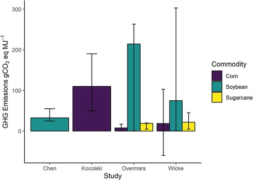
The consequences of uncertainty in future yield projections for calculated ILUC emissions from biofuels are profound (Figure 1). For example, Chen et al. (2018) found that factoring in a yield response to price reduced land clearing from soy biodiesel by 105%. Dumortier et al. (2010) found that including a yield-price response reduced Corn ethanol ILUC emissions from 1231 to 237 g CO₂ eq. MJ⁻¹. The extent of such parameter uncertainty caused Plevin et al. (2015) to advocate for probabilistic approaches as default in ILUC modelling and explicit presentation of uncertainty in all ILUC model results. The scale of uncertainty has also led to scepticism that current ILUC calculations should be used to inform policy (Plevin et al., 2017) and even whether mitigating ILUC emissions is an appropriate policy focus (Khanna et al., 2017).

Figure 1. Literature range for greenhouse gas emissions of 1^st generation biofuels: corn ethanol, soybean biodiesel and sugarcane ethanol, the predominant biofuel in Brazil (USDA FAS, 2019), which is included for context. In all studies ILUC is the principal cause of uncertainty. Chen and Kocolski are individual modelling studies, Wicke reviewed modelling studies, whilst Overmars used statistical methods. Error bars are full reported range. Sources: Chen – Chen et al. (2018); Kocolski – Kocolski et al. (2013); Overmars – Overmars et al. (2015); Wicke – Wicke et al. (2012)

Uncertainty about yield elasticity is complicated by contrasting accounts of the underlying processes driving yield growth. Economic studies of yield increases have tended to model yield over the long-term as a linear function of research and development spending (Baldos et al., 2018). Similarly, an analysis of the physiological basis of yield changes in soybean from 1920–2007 found a robust linear increase driven by gradual gains in photosynthetic efficiency and biomass allocation (Koester et al., 2014). However, other analyses have stressed the non-linear and disruptive impact of new agricultural technologies and policies on the land system. For example, studying the spatial allocation of land use change, Verstegen et al. (2016) found that increased demand for sugarcane ethanol in Brazil between 2003–2012 led to a fundamental shift in the land system between discrete system states.

Similarly, the introduction of genetically modified (GM) crops in 1996 has profoundly impacted agricultural production (Barrows et al., 2014a), further complicating our understanding of yield increases and their role in ILUC processes. Taheripour et al. (2016) reviewed literature on yield increases due to GM and found that, since their introduction, GM crops had driven a 5.2–17.1% increase in corn and 0–10.3% increase in soybean yields. GM crops had also greatly expanded the range of climatic conditions and soil types in which soybean can be grown by reducing competition pressures (Barrows et al., 2014a): Barrows et al. (2014b) found GM soybean had increased the acreage planted in the USA by up to 40%.

Previous studies of yield elasticity have typically used conventional statistical approaches such as linear and mixed-effects models to unpick the relative importance of factors influencing yields (e.g., Berry & Schlenker, 2011). However, these methods do not fully allow price-dependent yield changes to be separated from factors independent of price, which risks wrongful attribution of yield (in-)elasticity to exogenous factors such as climate or confusing the long-term rate of technological progress with short-term price-driven intensification (Golub & Hertel, 2012; study question one, as below). Furthermore, such methods do not support robust uncertainty quantification (study question two) and assume a yield elasticity that is static through time (study question three). To address these challenges, we take a novel approach to study of yield elasticities, by applying Bayesian network (BN) models. We discuss key aspects of BNs relevant to our study in section 2.1 and for a more detailed introduction readers are referred to online appendix 1.

Therefore, this study explores the impact of biofuel policies on yields in the USA corn and soybean production systems, which underpin creation of ethanol and biodiesel respectively. As the USA is the largest global producer of first-generation biofuels, and given BECCS remains an emerging technology, the USA is the best available test case to explore the potential ILUC consequences of BECCS. The study uses Bayesian network models to isolate yield response to price from confounding factors such as climate and long-term yield growth, to quantify uncertainty about yield elasticity, and to assess the impact of disruptive events on yields. It seeks to answer three central questions to better understand the importance of yield elasticity for ILUC:

1. Are USA corn and soybean yields elastic to price, and if so, to what extent?

2. What is an appropriate parameterisation to represent current uncertainty about yield elasticity within ILUC modelling studies?

3. Has yield elasticity shown discrete system shifts driven by new technologies (e.g., GM crops) or the introduction of biofuel policies? If not, has it evolved linearly or remained constant through time?

2. Methods

2.1. Overview of study methods

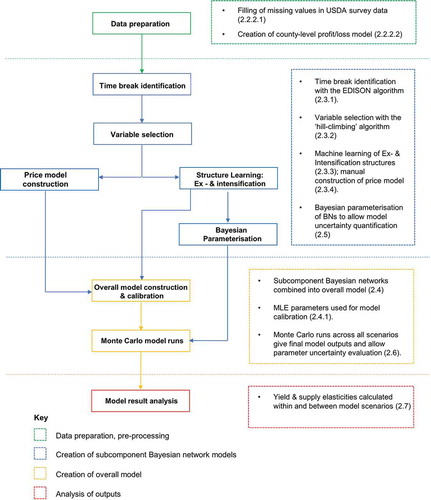
The structure of BNs can either be constructed using expert knowledge of a system, or using machine learning (Nagarajan et al., 2013). Typically, in the land use sciences, BN structures have been developed based on expert understanding (e.g., Celio et al., 2014), with the parameters of the model then defined quantitatively from field or remote sensing data (e.g., Nascimento et al., 2020). However, given the identified lack of literature agreement on the processes that drive yield increases, we adopt a machine learning approach to create network structures, thereby defining the presence (or absence) of relationships between variables numerically. Specifically, machine learning was used to create the structures of BN models for spatiotemporal subsections of the corn and soybean production systems (section 2.3). A flow chart of study methods is given in Figure 2.

Figure 2. Flowchart of study methods; numbers in parentheses in the accompanying text box indicate the paper section of corresponding descriptions in the text.

The use of BNs allowed relationships between price and agricultural intensification to be specified explicitly through the inclusion or omission of arcs (representing causal relationships) between price variables and drivers of yields (Figure 3). This should enable the price signal to be isolated from underlying yield growth (study question one, as above). The relationships represented by the arcs (directed edges) in a BN can themselves be parameterised with a probability distribution through Bayesian inference, enabling robust quantification of model parameter uncertainty (study question two; section 2.5).

Figure 3. Illustrative Bayesian network structure demonstrating separation of price-dependent from price-independent drivers of yield. Circles (nodes) represent variables and arrows (arcs) represent uni-directional probabilistic relationships between them (Jensen, 2001). The figure is an a-temporal static BN; by contrast a dynamic BN would factor in lagged responses between variables. Yield is influenced by two variables (termed ‘parent nodes’), one of which is price-dependent (e.g., rate of fertiliser application, b) and one is price-independent (e.g., growing season temperature, c). The price-dependent parent node to yield (b) can be updated given knowledge of price (a), allowing yield (d) to be predicted in the context of both price-dependent and price-independent variables (c).

To further isolate yield elasticity from other processes, intensification was defined as all farming decisions that impact yields on existing productive agricultural land – fertiliser, chemical, seed, machinery inputs and double cropping. Double cropping was included to account for the negative impact on yields of the late planting date required for a second crop (Mourtzinis et al., 2017). Extensification was included in the study to account for more marginal lands being brought into production and constraining yield elasticity under elevated prices (Secchi et al., 2009).

Methods developed in computational biology for the representation of gene regulatory networks with BNs support numerical identification of systemic breakpoints (Pyne et al., 2018). These methods simultaneously construct the dependencies within a system and compute the breakpoints at which these change significantly (Dondelinger et al., 2013). Such methods enabled identification of systemic shifts within US agricultural production during the study period (section 2.3.1). Identifying timesteps where structural changes in the land system occurred allowed relaxation of the assumption that yield elasticity is static through time (question three).

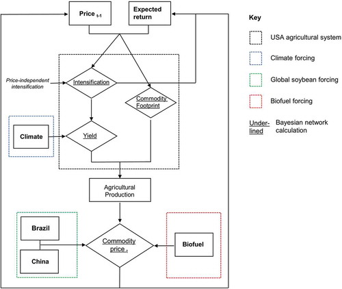
The resulting BN models of subsections of the overall study system were combined into a single holistic model (Figure 4; section 2.4). The USA soybean and corn agricultural systems were the central focus of the holistic model, with other drivers of commodity prices treated as external forcings. Varying these economic forcings was the basis of counterfactual experiments (section 2.6). Comparison of yields between scenarios allowed yield elasticity to be assessed (section 2.7). An erratic climate has been implicated in yield variance and agricultural commodity price spikes (Chatzopoulos et al., 2019). Therefore, whilst climate was not a central focus of counterfactual experiments, it was accounted for in intensification models, where yield was the target variable.

Figure 4. Structure of overall model. The USA agricultural system is the central model system, comprising 48 Bayesian Network sub-models. Commodity price is calculated with the two price BN models, using modelled national agricultural production and external forcings as inputs. The location of Bayesian networks in the overall model are indicated by underlined text.

2.2. Study boundaries and data processing

2.2.1. Study boundaries

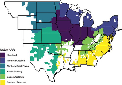
The study period was set as 1990–2017 to allow analysis of the impact on agricultural production of the introduction of biofuel mandates in 2005 and GM crops in 1996. The study focuses on USDA agricultural resource regions one to six (ARR) (US Department of Agriculture [USDA], 2000; Figure 5). The ARRs are areas of the USA with broadly similar agricultural land uses and production systems. ARRs one to six were chosen as these were the dominant corn and soybean regions during the study period, accounting for 97% and 91% of national production respectively (USDA, 2019); no data on key markers of intensification (machinery inputs, chemical and fertiliser inputs) were available for zones seven to nine (US Department of Agriculture Economic Research Service [USDA ERS], 2019).

Figure 5. Spatial boundaries of this study; only counties where data was available, and so were included in the analysis, are shown coloured in.

2.2.2. Data pre-processing

Table 1 gives an overview of sources and spatiotemporal resolution of data used in this study; Table 2 describes all candidate predictor variables in intensification, extensification and price BN models following data pre-processing. All data were re-scaled to an annual timestep and the county level, with linear interpolation used for data sets with partial spatial or temporal coverage. Where data were provided at the state-level, values for counties in missing states were filled with the mean of the relevant ARR. Processed data are made available as online appendices 2a-2 h, and a detailed overview of data pre-processing is given in appendix 3. Further key points are noted below.

Table 1. Overview of source, usage, temporal and spatial resolution of data sets used.

Dataset	Usage	Temporal extent (resolution)	Spatial resolution
USDA Agricultural Survey^a	Commodity acreage, yield, planting date, irrigated acreage	1990–2017 (Annual)	County
USDA ERS Intensification Data^b	GM adoption, fertiliser application rates, rate of chemical & machinery inputs	GM seed: 2000–2017 (Annual) Fertiliser application: 1990–2017 (Annual) Chemicals & Machinery: 1997–2017 (5-yearly)	State
USDA ERS Profit-Loss Model^b	Medium-term expected return per acre	1997–2017 (Annual)	Agricultural Resource Region
Conserve Reserve Programme Enrolment & Payments^c	CRP land availability and per acre payment	1990–2017 (Annual)	County
USDA agricultural insurance data^d	Medium-term expected return per acre, insured acreage pct.	1990–2017 (Annual)	County
USDA ERS agricultural subsidies^c	Feeds into medium-term expected return per acre	1990–2017 (Annual)	State
Climate data for continental USA^e	Mean growing season temperature and precipitation	1990–2017 (Monthly)	5 km^2 gridded
USDA ERS Biofuel Data^d	National level influence of biofuel price & production on underlying commodity price	1990–2017 (Annual)	National
USDA Foreign Agricultural Service Trade Data^f	Import and Export of Soybean & influence on price	1990–2017 (Annual)	National

Source:

^aUS Department of Agriculture [USDA NASS], 2019.

^bUSDA Economic Research Service [USDA ERS], 2019.

^cUSDA Farm Service Agency [USDA FSA], 2019.

^dUS Department of Agriculture Risk Management Agency [USDA RMA], 2019.

^eVose et al., 2014

^fUSDA Foreign Agricultural Service [USDA FAS], 2019.

Table 2. Overview of explanatory variables considered for inclusion in Bayesian network structures. Key: *raw acreage planted was for baseline data throughout, included as a proxy for the underlying suitability of the county for agriculture; ⁺nitrogen, potash and phosphate application rate considered separately.

Variable category	Extensification	Intensification
Economic variables	Pricet-1	Pricet-1
	Relative 3-year profit expectation between Corn, Soy and CRP lands	3-year profit expectation
	Proportion of total cropland planted with rice, sorghum, wheat or barley
Land management & suitability	Acres planted of target commodity (baseline)*	Acres planted of target commodity (baseline)*
	Change in acres planted of target commodity lag 1*	Rate of fertiliser^+, machinery and chemical application
	Total CRP lands	Julian Day at which half of target commodity was planted
		% of target commodity production irrigated
Climate	Growing season temperature	Growing season temperature
	Growing season precipitation	Growing season precipitation
GM uptake	Pre-GM acres planted of target commodity, % change in acres planted (1996 = 1)	GM uptake % for target commodity (overall and those with stacked attributes)
	GM uptake % for target commodity

2.2.2.1. USDA agricultural survey

The USDA agricultural survey provided core data for acreage planted and harvested, yield and percentage of planted acreage that was irrigated. Planting dates were used to calculate a day by when 50% of the crop had been planted, which has been suggested as a proxy for double cropping (Egli, 2008).

Response rates to the USDA Agricultural Survey are declining over time (Johansson & Effland, 2017). As a result, 61% of counties for soybean and 64% of counties for corn had at least one missing year of data. Survey responses are decreasing most acutely in regions outside Heartland (ARR one) – the region with the most intensive production and highest yields (USDA, 2019). For example, there were 10 times more missing data years per county in the Northern Great Plains (ARR three) compared to Heartland. Therefore, to mitigate this systematic bias, all counties with at least two data points were included, with linear interpolation used to fill missing years. The impact of this on study results were evaluated by learning BN models on data both with and without this data cleaning.

2.2.2.2. County-level price and profit margin

Farmers’ decisions on which crops to grow, and how intensively, are influenced by short-term commodity prices and climate anomalies (Schnitkey & Zulauf, 2019), tempered substantially by government subsidies (Graff Zivin & Perloff, 2012) and insurance schemes (Babcock, 2012). However, a thorough and recent account of the weight farmers ascribe to these factors during their decision making could not be identified. Therefore, economic influence on land use was modelled in two ways, representing different weights to this information. Both representations of economic decision-making become candidate predictor variables in a single set of extensification and intensification model structures (Table 2).

The first method, to represent a short-term or low-information decision, was simply to allow commodity price from the previous year to influence decision-making in the following year. Small regional differences in farm gate prices were ignored as price in the overall model was calculated at a national level (section 2.4). Second, to represent a higher-information decision, USDA ERS calculations of profit per-acre (USDA ERS, 2019) were used as the basis for a per-acre profit-loss calculation for both corn and soybean. This accounted for yield, commodity price, operation and capital costs, crop failure, subsidies, insurance payments and the opportunity cost (the unrealised potential value of labour if put to another productive use) of using land productively rather than fallowing land and acquiring subsidies under the Conservation Reserve Programme (CRP) over a three-year window. For a detailed description see online appendix 3.

2.3. Component model construction

Prior to model construction, data were divided into the six USDA ARRs. Each region was then treated as a separate spatial subsystem. The target variable (the variable of central interest in a BN) for the intensification subnetworks was yield, and for extensification BNs the target was the change in acreage from the prior year.

2.3.1. Time break identification

Growth in biofuel demand was previously found to cause discrete system shifts in land use (Verstegen et al., 2016). Therefore, we employed the EDISON machine learning algorithm (Dondelinger et al., 2013, appendix 1) to identify years in which systems exhibited a systemic shift. All potential explanatory and target variables were passed to the algorithm, which was run over 100 bootstrap samples of data for each ARR. To avoid overfitting resulting from multiple breakpoints being identified in consecutive study years, a single time break was permitted per spatial subsystem. The modal year identified as the highest probability breakpoint across iterations was chosen. This created 12 spatiotemporal subsystems of extensification and intensification for each commodity.

2.3.2. BN variable selection

An initial screening of predictor variables (termed ‘feature selection’ in machine learning) was conducted to encourage parsimonious model learning. Within the time breaks identified by the EDISON algorithm, network structures were created using the ‘hill climbing’ machine learning approach (Nagarajan et al., 2013), which creates network structures by seeking to optimise a given metric (appendix 1). The algorithm was run across 1000 bootstrap iterations with the Bayesian Information Criterion (BIC) as the metric (Schwarz, 1978). Variables were retained if they connected to the target variable in at least 50% of network structures.

2.3.3. BN structure and parameter learning

Following variable selection, network structures for extensification and intensification were constructed using the same bootstrap hill-climbing machine learning approach. To enable the final network structures to appropriately represent causal processes in the system, physically meaningless arcs (such as from yield to climate) were blacklisted from consideration by the algorithm. Furthermore, having identified temporal breakpoints in the system, static (a-temporal) BNs were used for model construction (Figure 3). An assumption of dynamic BNs is that all variables potentially have lagged relationships. However, to best represent prior knowledge about farmers’ decision-making, we elected to directly specify which variables could exhibit lagged relationships. Therefore, we adopted a static BN framework, and defined lag structures explicitly by including price from the previous year and our profit-loss model as candidate predictor variables. A summary of the lagged relationships included in the model is given in Table 3.

Table 3. Summary of temporal dependencies allowed between variables in BN models. Relative expected return is the expected return between soybean and corn, and between each commodity and CRP payments. Change in commodity acreage at lag 1 represents the effects of crop rotation on commodity acreage (Plourde et al., 2013).

Variable	Time lag (years)	Intensification	Extensification
Change in commodity acreage	1	✗	✓
Commodity price	1	✓*	✓
Expected return on production	1–3	✓*	✓
Relative expected return	1–3	✗	✓

* Price lags influence yield through intermediary variables such as fertiliser inputs.

A range of arc selection thresholds based on the proportion of bootstrap iterations in which an arc was present were then trialled. Therefore, to enable model assessment, data for 20% of counties were held back as a testing set. Final network structures were selected based on their overall BIC score and the RMSE of predictions on the relevant target variable in the testing set. Predictions from BNs were conducted using ‘likelihood weighting’ throughout; this is a stochastic sampling method for prediction that uses all available evidence in a BN, not just the direct parents of a node, and therefore accounts for indirect relationships in a system (Guo & Hse, 2002; see appendix 1).

The chosen library for BN modelling, ‘bnlearn’ (Scutari, 2010; section 2.8), has best-in-class facility for machine learning of network structures in systems with both discrete and continuous data types (Nagarajan et al., 2013). However, it does not support Bayesian parameterisation of such networks. Therefore, parameters for the relationships between nodes were initially specified with maximum likelihood estimates, which were used for model selection and calibration of the overall model. These parameters were then relearned with Bayesian methods to allow uncertainty quantification in model experiments (section 2.5).

2.3.4. Price model construction

For price models, only 28 data points were available as training data. Therefore, rather than using machine learning to develop model structures, price BN models were constructed manually based on subject-matter knowledge and predictive accuracy. Final models were selected on the RMSE of their predictions across all 28 data points.

2.4. Overall model construction

The 50 resulting BN models (12 intensive and 12 extensive component models, plus one price model, for each commodity) were then combined into one comprehensive model (Figure 4). Farmers’ extensification and intensification decisions were predicted simultaneously at each time step. Based on intensive inputs, yield was predicted. Yield and commodity footprint predictions were combined to calculate agricultural production of each commodity. To convert production in the six study ARRs to national production, modelled production was multiplied by the reciprocal of the ratio of production in the study area to national production in USDA data in each study year:

(1) ${\widehat{Production}}_{National,t}=\sum _{n=1}^{n=6}{\widehat{Production}}_{n,t}\ast \frac{1}{Productio{n}_{ARR1-6,t}/Productio{n}_{National,t}}$(1)

Modelled national production was then fed into the models of corn and soybean price. Calculated price became the lagged price variable influencing production in the next year. Modelled price and yield were also used to update three-year expected return, with costs scaling linearly with the percentage change in modelled inputs against baseline data. The difference between expected return from corn, soybean, and CRP payments was also updated.

2.4.1. Model calibration

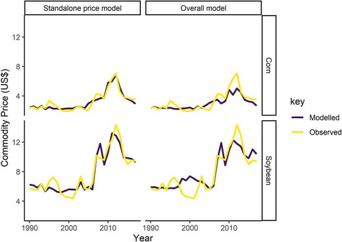
Intensification and extensification outputs of the overall model were calibrated using annual county-level USDA yield and acreage data. During this process, extensification BNs consistently overestimated the elasticity of commodity acreage to price. Therefore, predicted change in acreage was divided by a free parameter representing the economic cost of converting new farmland for production (Claasen & Tegene, 1999). The available acreage in each county was restricted to 150% of the maximum commodity acreage in the underlying data. With these additional constraints, the model performed well against observations (soybean pseudo r² = 0.78, corn pseudo r² = 0.79). Prices in the baseline runs were an average of 2.51% above modelled prices in the standalone price model, and an average of 3.21% below this reference price in corn, suggesting the overall model slightly underestimated (overestimated) soybean (corn) supply elasticity (Figure 6). Importantly, for both commodities, the model overestimates supply elasticity during the acute 2012 price spike.

Figure 6. Model calibration showing predicted price in the overall model and the price models as a standalone using observed production data. Additional error in the overall model outputs is therefore caused by errors in modelled USA agricultural production. Whilst both models perform well against observations, for both commodities, the overall model overestimates farmers’ capacity to respond to increased price pressure during the 2012 commodity spike.

2.5. Uncertainty quantification

In addition to assessment of data uncertainty on BN model structures (section 2.2.2.1), parameter uncertainty was assessed. Deterministic parameters for each node in all intensification and extensification BNs were replaced with parameter distributions derived from Bayesian regressions. Where both discrete and continuous variables were present, separate parameter distributions were computed for each combination of discrete nodes in the network structure. This process was the direct Bayesian equivalent of the frequentist approach used to derive the BNs’ original deterministic parameters (Scutari, 2010). Weakly informative priors, specifying the type of the posterior distribution (e.g., normal, gamma, etc.) without imparting strong information on its parameter values, were used for all variables in each regression (Gelman et al., 2008). These were normal distributions with µ = 0 and σ as follows:

(2) ${\sigma }_{intercept}=10\ast \sigma \left(y\right)$(2)

(3) ${\sigma }_{coefficient}=\left(2.5/\sigma \left(x\right)\right)\ast \sigma \left(y\right)$(3)

Probability-weighted samples (n = 500) were then made from the resulting posterior distributions to enable Monte Carlo simulation of the overall model. Whilst results presented for the overall model exclusively use stochastic intensification and extensification models, price models remained deterministic.

2.6. Model experiments

Four counterfactual scenarios of the study period were explored to assess yield elasticities given shifts in economic forcings. These were compared against a baseline run where all forcings used historical values from USDA ERS data (USDA ERS, 2019). The counterfactuals were: ‘Double Biofuel’ and ‘Half Biofuel’ in which forcings for biofuels were doubled and halved respectively; and ‘Double Both’ and ‘Half Both’ in which both biofuel and Chinese soybean demand were doubled and halved respectively.

2.7. Analysis of results

Calculation of inter-scenario elasticity allowed the reaction of yields to the underlying demand signal to be isolated from other confounding factors. First, percentage change in yield between each scenario and the baseline run in each study year was calculated. Second, change in demand was calculated as the percentage change between baseline price and the theoretical price with increased demand but static supply predicted from standalone BN price models:

(4) $\widehat{Elasticity}=\frac{Yiel{d}_{scenario}-Yiel{d}_{baseline}}{Yiel{d}_{baseline}}/\frac{{\widehat{Demand}}_{scenario}-{\widehat{Demand}}_{baseline}}{{\widehat{Demand}}_{baseline}}$(4)

2.8. Computational tools

Data preparation, modelling and analysis were conducted with the R programming language version 3.6.1 (R Foundation for Statistical Computing, 2019). Time breaks were identified using EDISON library version 1.1.1 (Dondelinger et al., 2013). BN models were constructed using the bnlearn package version 4.4.1 (Scutari, 2010). Bayesian parameter learning for BN models was conducted in RStanarm version 2.18.2 (Goodrich et al., 2018). Project code and R objects used to run the final model, including all 50 BN structures used, are made available as online appendices 4a-4 c.

3. Results

3.1. Component models

3.1.1. Time breaks

Temporal breakpoints identified numerically by the EDISON algorithm show clear alignment with real-world disruptive events (Table 4), suggesting this method identified meaningful systemic shifts in the study system. Breakpoints for extensification all align with the introduction of GM crops, whilst 11/12 soybean and corn breakpoints cluster around the 2005 introduction of biofuel mandates and the 2012 commodity price spike.

Table 4. Breakpoint years identified for each commodity subsystem.

Agricultural Resource Region	Soybean Acreage	Corn Acreage	Soybean Intense	Corn Intense
Heartland	1996	1996	2005	2013
Northern Crescent	1996	1996	2013	2013
Northern Great Plains	1996	1996	2005	2006
Prairie Gateway	1996	1996	2005	2006
Eastern Uplands	1996	1996	2013	2013
Southern Seaboard	1996	1996	1992	2013

3.1.2. Price models

The best-performing model of corn price had two predictor variables: USA production and the product of corn ethanol price and proportion of USA corn production used for ethanol (pseudo r² = 0.90). The best-performing model of soybean price had three predictor variables: USA production, the price of biodiesel and Chinese soybean imports minus Brazilian soybean production – reflecting the importance of the globalised trading of soybean meal as animal feed in the commodity system (pseudo r² = 0.90; Yao et al., 2018).

3.1.3. Underlying drivers of yields

Analysis of BN structures shows the primary influence on yields for both commodities are intensive inputs, accounting for 66% of parent nodes to yield in corn and 55% in soybean. ‘Parent nodes’ are those that influence a given variable of interest (Figure 3). GM crops play a larger role in corn yields (13 parent nodes across all networks; Figure 7) than soybean yields (3 parent nodes). Soybean is more sensitive to climate, with growing season temperature and precipitation accounting for 38% of parent nodes to yield, compared to 20% in corn. Yield is more closely linked to price variables in corn, which had 45 price-dependent intensive drivers of yield, to 27 in soybean (Figure 8).

Figure 7. Frequency of intensive agricultural inputs as parent nodes to yield in Bayesian network structures. ‘Interpolated’ and ‘Filtered’ reflect the two approaches trialled to deal with missing values in the underlying USDA data.

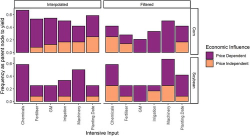
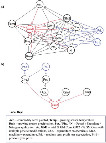
Figure 8. Example Bayesian network model structures used in this study: a) for corn intensification in Heartland from 1990–2012 and b) for soybean intensification in the Northern Great Plains from 2005–2017. Yield and its relationships with other variables are marked red, whilst price variables and their relationships are marked blue. a) is denser, with a larger range of variables influencing yield, and more of these being influenced by price, whereas b) shows a greater impact for underlying environmental factors.

However, comparison of networks learned on data with linear interpolation across missing values (hereafter ‘interpolated data’) to those learned on data where counties with poorer data quality were filtered (hereafter ‘filtered data’) questions the certainty of these findings. In contrast to networks based on the interpolated data, networks for the filtered data have a similar number of intensive inputs as parents to yield between commodities: 35 for corn and 33 for soybean.

Corn networks for Heartland (ARR1), where data was most complete, had just one fewer parent node yield for intensive inputs in the filtered data than the interpolated data. However, overall there were 26% fewer intensive inputs as parent nodes to yield in the filtered data compared to the interpolated data. In contrast, in soybean there was one more intensive input as a parent to yield in the filtered data, but there were four fewer parent nodes related to climate. This is indicative of the filtered data being weighted towards more established agricultural regions, where yields were less climate-dependent.

3.2. Overall model

3.2.1. Overview of model outputs

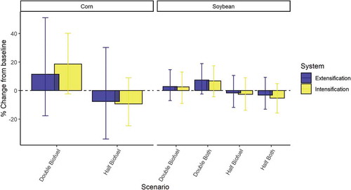
Model results indicate the agricultural system is substantially responsive to price effects (Figure 9). Doubling of biofuel forcing leads to a 20.63% increase in corn yield and the ‘double both’ scenario leads to a 6.97% increase in soybean yields from the mean annual values across baseline scenario runs. In corn, intensification is more responsive to changes in demand than extensification by an average of 42.50%. Furthermore, price effect sizes are far greater in corn than soybean, perhaps reflecting the stronger role of climate in the soybean system. However, in all cases, the 95% confidence interval is greater than the effect size, indicative of substantial parameter uncertainty across models of both commodities.

Figure 9. Intensive and extensive response of agricultural production to changes in economic forcings. Columns are median values; error bars are 95% confidence interval.

3.2.2. Yield elasticity

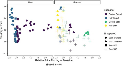
Calculating relative yield elasticity between counterfactual scenarios provides point estimates of 0.223 for corn and 0.152 for soybean (Table 5, Figure 10). Yield elasticity was significantly greater than zero in all scenarios (one-way Wilcoxon-tests: corn, p <0.0001; soybean p <0.0001). Yield elasticity was significantly larger in scenarios where demand was decreased than in scenarios where demand was increased (one-way Kolmogorov-Smirnov tests, both commodities p <0.0001). This trend was most stark in the soybean biofuel only scenarios: median elasticity was just 0.065 in double biofuel, but 0.171 in half biofuel. Furthermore, yield elasticity tended to be negatively correlated with increased price forcing against the baseline. This trend was present throughout in soybean (Kendall’s Tau: $\tau$ −0.20, p <0.0001), but only present in corn after the introduction of biofuel mandates in 2005 (−0.29, p <0.0001); before this the relationship was weakly positive ($\tau$ +0.18, p <0.0001).

Table 5. Summary statistics for relative yield elasticity between counterfactual scenarios and baseline model runs. Biofuel only and biofuel + Chinese demand scenarios for soybean are combined by respective increase or decrease in forcing.

		Corn			Soybean
Percentile	Overall	Double Forcing	Half Forcing	Overall	Double Forcing	Half Forcing
25^th	0.111	0.113	0.110	0.045	0.028	0.083
50^th	0.223	0.206	0.256	0.152	0.109	0.199
75^th	0.349	0.286	0.458	0.287	0.223	0.383

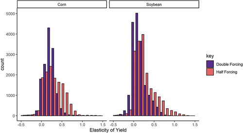
Figure 10. Relative yield elasticity between counterfactual and baseline scenarios from Monte Carlo simulation. Results are grouped by scenarios where biofuel and Chinese soybean demand forcings were increased (double forcing) or reduced (half forcing). Values below 0 are indicative of a high degree of parameter uncertainty in the model. Although positively skewed (skewness: corn 0.019; soybean 0.812), overall commodity distributions are closer to a normal than lognormal distribution. Counts are of national mean elasticity in a given simulation study year.

Yield elasticity showed clear evidence of systemic shifts in response to price events in both corn and soybean (Figure 11). Yield elasticities in corn after the introduction of biofuel mandates in 2005 increased by 156%, and after the commodity price spike in 2012 soybean yield elasticities increased by 87% (one-way Kolmogorov-Smirnov tests, both p <0.0001). This suggests these major economic events more closely couple the system to price, although the larger effect size in scenarios with reduced demand pressures suggests the size of the event strongly impacts the system’s ability to respond (Table 6). Importantly, the combination of the negative correlation of yield elasticity with increasing price pressure and increased yield elasticity post-2005 entails that when model outputs for the half biofuel run in corn from 2005 onwards are excluded, corn yield elasticity drops to 0.13 – giving a roughly similar value to soybean.

Table 6. Change in relative yield elasticity against the baseline scenario up to and after the given time break years. Overall, the 2005 introduction of biofuel mandates, and the 2012 commodity price spike serve to increase the impact of short-term economic factors on yields. Soy biodiesel only became a major influence on soybean prices after 2005, so data from before that point are not shown.

Time break	Scenario	Soybean	Corn
2005	Double Biofuel	-	0.115
2012	Double Biofuel	0.235	0.113
2005	Half Biofuel	-	0.321
2012	Half Biofuel	0.469	0.219
2005	Double Both	−0.135	-
2012	Double Both	−0.027	-
2005	Half Both	0.028	-
2012	Half Both	0.203	-

Figure 11. Scatter plots of relative yield elasticities between counterfactual scenarios and baseline runs. Non-linear system shifts are highlighted by plotted shape. Soybean biofuel scenarios are shown from 2008 when biodiesel began to play a significant role in USA soybean production.

4. Discussion and conclusions

4.1. Implications for ILUC modelling

In the results presented here, yield elasticity was greater than zero in all scenarios and across all time periods, reinforcing the findings of previous studies that intensification is vital for determining ILUC emissions. Point estimates for yield elasticities of 0.223 for corn and 0.152 for soybean are in broad agreement with the majority view in the literature for values of this parameter (Table 7). The results in this study do not support the findings of Berry (2011) that yield is uncoupled from price effects, but do bolster that study’s argument that the widely used 0.25 value is a substantial overestimate (Hertel et al., 2010).

Table 7. Yield elasticity results compared to literature values. The value for Laborde and Valin (2011) is for all crops in the USA.

Commodity	This study	Berry, 2011	Huang & Khanna, 2010	Hertel et al., 2010	Laborde & Valin, 2011
Corn	0.223 (0.136^+)	0.03	0.15	0.25	0.2
Soybean	0.152 (0.133^+)	-	0.06	-	0.2

^{+ parameter value when substantial elasticities projected in the reduced forcing scenarios are filtered from the data.}

However, several factors complicate these findings. In our results, yields are clearly more elastic when demand declines than when demand increases (Figure 10). Declining yield elasticity as price pressure increases is particularly evident in corn after the introduction of biofuels and suggests farmers’ ability to increase yields in response to price has strong limitations. Using a single value to parameterise yield elasticity in ILUC modelling risks failing to capture this fundamental aspect of the system.

This result is particularly notable given the model’s overestimation of supply elasticity during the 2012 commodity spike (Figure 6). Although, the processed data included variables reflecting the relative expected profit of growing soybean or corn in extensification models (Table 2), such nodes were rarely adopted during structure learning. Therefore, fully accounting for competition for available land between commodities is a limitation of the model presented, which contributed to the overestimation of supply elasticity during the 2012 price shock. As Bayesian networks gain traction in the land use sciences, future studies should pay careful attention to how such models can most effectively represent spatially-dependent competition between commodities, human land use decisions and evaluation of trade-offs.

In line with the findings of Verstegen et al. (2016), results here show that yield elasticity shifts between discrete system states coincident with major price events – primarily the 2005 introduction of biofuel mandates in the case of corn and the 2012 commodity spike in the case of soybean. It is likely that capital investment has played a role in this process. USDA data shows machinery investment in both corn and soybean spiked by more than 30% between 2011 and 2012, suggesting substantially higher prices were driving additional investment and enabling higher yields. This factor, combined with the observed decreasing elasticity with increased forcing points to a ‘goldilocks window’ for yield elasticity: enough price increase to justify one-off capital outlays, not too large such that farmers lack the technology to respond.

The role of capital investment also questions how durable yield gains due to increased intensive inputs would be in a period of prolonged lower demand (Bellmann & Hepburn, 2018). Whilst corn ethanol prices declined by 103% and soy biodiesel prices declined by 38% from 2012–2017 (USDA ERS, 2019), the introduction of the ARC subsidy scheme, which uses a five-year average to determine a baseline commodity price, has meant that the 2012 price spike continued to influence production until 2017 (USDA ERS, 2019). Discussion of whether yield increases due to farmer-driven intensification are permanent or reversible is severely limited in the literature (see Malins et al. (2014) for a summary), and this study suggests more work is needed in this area. Furthermore, the importance of major price events to the system combined with the complexity of the subsequent yield response indicates land use models treating yield increase as a linearly increasing exogenous forcing may not be equipped to robustly capture the dynamics of ILUC processes.

Whilst it was possible to detect systemic shifts in the land system due to national-scale price events, the central limitation of our study was that data uncertainty confounded precise conclusions regarding the underlying drivers of yield elasticity – a multi-faceted process that plays out in complex ways at the county-scale. Yield elasticity is inherently uncertain due to more limited data availability than for extensification for which satellite data allow ready quantification (e.g., Boryan et al., 2011). Future work should focus on primary data gathering via field studies and farm-level surveys or development of novel remote sensing methods to further advance knowledge of the processes that determine farmers’ ability to respond to prices through intensification.

The importance of singular price events to the agricultural system during the study period questions whether probabilistic modelling on its own can capture a representative range of future ILUC scenarios. In addition to biofuels, increased agricultural commodity price variance has been linked to multiple exogenous drivers broadly indicative of increased globalisation, such as spillovers between agricultural and energy markets, futures’ trading and exchange rate policies (Grosche & Heckelei, 2016; Kalkuhl et al., 2016). In future, studies involving scenario-based ILUC modelling should incorporate the varying probability of trade disruptions and resulting system shocks under different socioeconomic pathways (Kalkuhl et al., 2016; O’Neill et al., 2014). The telecoupling framework may provide a conceptual basis to implement this in a systematic way (Liu et al., 2013). Further, the extent of parameter uncertainty in these results (Figure 9) reiterates the need for all ILUC studies to use probabilistic approaches as standard (Plevin et al., 2015).

4.2. Implications for policy

This study’s most immediate policy implication is that biofuel policies informed by studies which parameterised yield elasticity with a single value in the commonly used range of 0.2–0.25 may underestimate ILUC effects and overestimate the reductions in greenhouse gas emissions from first-generation biofuels. For example, assessments of the US National Renewable Fuel Standard and California’s Low Carbon Fuel Standard assumed a uniform yield elasticity of 0.25 (Hoekman & Broch, 2018). More fundamentally, the limitations of a single deterministic parameter for yield elasticity illustrated here further questions whether ILUC is currently understood and quantified to a precision that provides an appropriate basis for effective ILUC mitigation policies (Khanna et al., 2017; Pelkmans et al., 2019).

Systemic shifts due to price events combined with greater yield elasticity when prices decline in the results here are consistent with a conceptual model of yield elasticity in which farmers may use intensive inputs to increase yield to a limited degree in the short-term, but where larger yield increases are ultimately a function of agricultural technology. Therefore, as farmers have relatively recently made substantial capital investments to respond to higher prices in the USA, it is unclear whether technology has advanced enough to enable US farmers to respond to a further system shock from the proposed increased biofuel mandate (Hoekman & Broch, 2018).

Such a strong limit to upside yield elasticity also highlights the potential for one-off price spikes to create vulnerabilities for terrestrial Carbon stocks through peaks in ILUC emissions (Grosche & Heckelei, 2016). Price spikes present an inherent difficulty for payment-based conservation schemes such as the US Conservation Reserve Programme (CRP), as rapid price changes can outpace policy responses such as increased conservation payments (Wright & Wimberley, 2013). This challenge reflects a growing concern that lack of consideration of lagged-responses between the multiple actors in the land system risks undermining climate change mitigation policy-making (Brown et al., 2019). Therefore, to avoid land use emissions and damage to biodiversity (Wimberley et al., 2017), payments in the CRP and similar schemes elsewhere may need to be pre-emptively increased before any future subsidies or mandates to promote biofuel production are introduced.

The potential for price spikes may increase as the currently regionalised production and consumption of biofuels becomes increasingly globalised (Matzenberger et al., 2015). However, the introduction of cellulosic biofuels may loosen the linkage between fuel prices and food inherent to first generation biofuels (Janda & Kristoufek, 2019), potentially mitigating against future price spikes. This bolsters the case for governments to incentivise cellulosic biofuel research and deployment rather than increasing existing mandates and subsidy schemes (Robertson et al., 2017). Moreover, for the carbon removal potential of BECCS to be realised, not only will supply chains need to be energy efficient (Fajardy & Mac Dowell, 2018), but also robustly future-proofed against price spikes and peaks in ILUC emissions.

Data availability

The data and code that support the findings of this study are openly available via figshare at https://doi.org/10.6084/m9.figshare.c.4805667.

Acknowledgments

We would like to acknowledge the contribution of Jeroen Keppens of King’s College London Department of Informatics for his useful advice on machine learning of Bayesian network models. Any errors are the responsibility of the authors.

Disclosure statement

The authors disclose no conflict of interest.

Correction Statement

This article has been republished with minor changes. These changes do not impact the academic content of the article.

Additional information

Funding

This work was supported by the UK Natural Environment Research Council, under grant reference NE/M021548/1.

References

- Babcock, B. (2012). The politics and economics of the US crop insurance program. In J.S. Graff Zivin & J.M. Perloff (Eds.), The intended and unintended effects of US agricultural and biotechnology policies (pp. 83–112). University of Chicago Press.
- Baldos, U., Viens, F., Hertel, T., & Fuglie, K. (2018). R&D spending, knowledge capital and agricultural productivity growth: A Bayesian approach. American Journal of Agricultural Economics, 101(1), 291–310. https://doi.org/10.1093/ajae/aay039
- Barrows, G., Sexton, S., & Zilberman, D. (2014a). Agricultural biotechnology: the promise and prospects of genetically modified crops. Journal of Economic Perspectives, 28(1), 99–120. https://doi.org/10.1257/jep.28.1.99
- Barrows, G., Sexton, S., & Zilberman, D. (2014b). The impact of agricultural biotechnology on supply and land-use. Environment and Development Economics, 19(6), 676–703. https://doi.org/10.1017/S1355770X14000400
- Bellmann, C., & Hepburn, J. (2017). The decline of commodity prices and global agricultural trade negotiations: A game changer? [online]. International Development Policy, 8(1). https://doi.org/10.4000/poldev.2384
- Berry, S. (2011). Biofuels policy and empirical inputs to GTAP models (Report to the California Air Resources Board). Yale University. https://ww3.arb.ca.gov/fuels/lcfs/workgroups/ewg/010511-berry-rpt.pdf
- Berry, S., & Schlenker, W. (2011). Empirical evidence on crop yield elasticity (Technical Report for the ICCT). International Council on Clean Transportation. https://theicct.org/sites/default/files/publications/berry_schlenker_cropyieldelasticities_sep2011.pdf
- Boryan, C., Yang, Z., Mueller, R., & Craig, M. (2011). Monitoring US agriculture: The US department of agriculture, national agricultural statistics service, cropland data layer program. Geocarto International, 26(5), 341–358. https://doi.org/10.1080/10106049.2011.562309
- Brown, C., Alexander, P., Arneth, A., Holman, I., & Rounsevell, M. (2019). Achievement of Paris climate goals unlikely due to time lags in the land system. Nature Climate Change, 9(3), 203–208. https://doi.org/10.1038/s41558-019-0400-5
- Celio, E., Koellner, T., & Gret-Regamey, A. (2014). Modelling land use decisions with Bayesian networks: Spatially explicit analysis of driving forces on land use change. Environmental Modelling and Software, 52, 222–233. https://doi.org/10.1016/j.envsoft.2013.10.014
- Chatzopoulos, T., Dominguez, I., Zampieri, M., & Toreti, A. (2020). Climate extremes and agricultural commodity markets: A global economic analysis of regionally simulated events. Weather and Climate Extremes, 27(100193). https://doi.org/10.1016/j.wace.2019.100193
- Chen, R., Qin, Z., Han, J., Wang, M., Taheripour, F., Tyner, W., O’Connor, D., & Duffield, J. (2018). Life cycle energy and greenhouse gas emission effects of biodiesel in the United States with induced land use change impacts. Bioresource Technology, 251, 249–258. https://doi.org/10.1016/j.biortech.2017.12.031
- Claasen, R., & Tegene, A. (1999). Agricultural land use choice: A discrete choice approach. Agricultural Resources and Economic Reviews, 28(1), 26–36. https://doi.org/10.1017/S1068280500000940
- Dondelinger, F., Lebre, S., & Husmeier, D. (2013). Non-homogeneous dynamic Bayesian networks with Bayesian regularization for inferring gene regulatory networks with gradually time-varying structure. Machine Learning, 90(2), 191–230. https://doi.org/10.1007/s10994-012-5311-x
- Dumortier, J., Hayes, D., Carriquiry, M., Dong, F., Du, X., Elobeid, A., Fabiosa, J., & Tokgoz, S. (2010). Sensitivity of carbon emission estimates from indirect land-use change. Applied Economic Perspectives and Policy, 33(3), 428–448. https://doi.org/10.1093/aepp/ppr015
- Egli, D. (2008). Soybean yield trends from 1972 to 2003 in mid-western USA. Field Crops Research, 106(1), 53–59. https://doi.org/10.1016/j.fcr.2007.10.014
- El Akkari, M., Réchauchère, O., Bispo, A., Gabrielle, B., & Makowski, D. (2018). A meta-analysis of the greenhouse gas abatement of bioenergy factoring in land use changes [online]. Scientific Reports, 8(8563). https://doi.org/10.1038/s41598-018-26712-x
- Fajardy, M., Koberle, A., MacDowell, N., & Fantuzzi, A. 2019. BECCS deployment: A reality check (Grantham Institute Briefing paper No 28). https://www.imperial.ac.uk/media/imperial-college/grantham-institute/public/publications/briefing-papers/BECCS-deployment---a-reality-check.pdf
- Fajardy, M., & Mac Dowell, N. (2018). The energy return on investment of BECCS: Is BECCS a threat to energy security? Energy & Environmental Science, 11(6), 1581–1594. https://doi.org/10.1039/C7EE03610H
- Fuchs, R., Alexander, P., Brown, C., Cossar, F., Henry, R., & Rounsevell, M. (2019). Why the US-China trade war spells disaster for the Amazon. Nature, 567(7749), 451–454. https://doi.org/10.1038/d41586-019-00896-2
- Gelman, A., Jakulin, A., Pittau, M., & Su, Y. (2008). A weakly informative default prior distribution for logistic and other regression models. The Annals of Applied Statistics, 2(4),1360–1383. https:/doi.org/10.1214/08-AOAS191
- Golub, A., & Hertel, T. (2012). Modelling land-use change impacts of biofuels in the GTAP-BIO framework. Climate Change Economics, 3(3), 1250015‐1–1250015‐30. https://doi.org/10.1142/S2010007812500157
- Goodrich, B., Gabry, J., Ali, I., & Brilleman, S. (2018). Rstanarm: Bayesian applied regression modelling via Stan (version 2.17.4). http://mc-stan.org/.
- Gough, C., Garcia-Freites, S., Jones, C., Mander, S., Moore, B., Pereira, C., Röder, M., Vaughan, N., & Welfle, A. (2018). Challenges to the use of BECCS as a keystone technology in pursuit of 1.5⁰C. Global Sustainability, 1(5), 1–9. https://doi.org/10.1017/sus.2018.3
- Graff Zivin, J., & Perloff, J. (2012). Editorial introduction to the intended and unintended effects of US agricultural and biotechnology policies. University of Chicago Press.
- Grosche, S., & Heckelei, T. (2016). Directional volatility spillovers between agricultural, crude oil, real estate, and other financial markets. In M. Kalkuhl, J. von Braun, & M. Torero (Eds.), Food price volatility and its implications for food security and policy (pp. 182–207). Springer.
- Guo, H., & Hse, W. (2002). A survey of algorithms for real-time bayesian network inference. In AAAI/KDD/UAI joint workshop on realtime decision support and diagnosis systems. American Association of Immunologists. [online] https://www.aaai.org/Papers/Workshops/2002/WS-02-15/WS02-15-001.pdf
- Hertel, T., Golub, A., Jones, A., O’Hare, M., Plevin, R., & Kammen, D. (2010). Effects of US maize ethanol global land use and greenhouse gas emissions: Market-mediated responses. BioScience, 60(3), 223–231. https://doi.org/10.1525/bio.2010.60.3.8
- Hertel, T., West, A., Borner, J., & Villoria, N. (2019). A review of global-local-global linkages in economic land-use/cover change models [online]. Environmental Research Letters, 14(5), 053003. https://doi.org/10.1088/1748-9326/ab0d33
- Hoekman, G., & Broch, S. (2018). Environmental implications of higher ethanol production and use in the US: A literature review. Part II – Biodiversity, land use change, GHG emissions and sustainability. Renewable and Sustainable Energy Reviews, 81(2), 3159–3177. https://doi.org/10.1016/j.rser.2017.05.052
- Huang, H., & Khanna, M. (2010). An econometric analysis of U.S. crop yield and cropland acreage: Implications for the impact of climate change [Paper presentation]. 2010 Annual Meeting of the Agricultural and Applied Economics Association, Denver Colorado. https://ideas.repec.org.
- Intergovernmental Panel on Climate Change (2018). Global warming of 1.5°C (IPCC Special Report No. 15). IPCC. https://www.ipcc.ch/sr15/
- Janda, K., & Kristoufek, L. (2019). The relationship between fuel and food prices: Methods, outcomes, and lessons for commodity price risk management (Working Paper No. 20/2019). Centre for Applied Macroeconomic Analysis. https://doi.org/10.2139/ssrn.3336355
- Jensen, F. (2001). Bayesian networks and decision graphs. Springer.
- Johansson, R., & Effland, A. (2017). Falling response rates to USDA crop surveys: Why it matters. University of Illinois. https://farmdocdaily.illinois.edu/
- Kalkuhl, M., von Braun, J., & Torero, M. (2016). Volatile and extreme food prices, food security and policy: An overview. In J. von Braun, M. Kalkuhl, & M. Torero (Eds.), Food price volatility and its implications for food security and policy (pp. 3–35). Springer.
- Kenney, R., & Hertel, T. (2009). The indirect land use impacts of United States Biofuel policies: The importance of acreage, yield, and bilateral trade responses. American Journal of Agricultural Economics, 91(4), 895–909. https://doi.org/10.1111/j.1467-8276.2009.01308.x
- Khanna, M., Wang, W., Hudiburg, T., & DeLucia, E. (2017). The social inefficiency of regulating indirect land use change due to biofuels. Nature Communications, 8(1), 15513. https://doi.org/10.1038/ncomms15513
- Kocolski, M., Mullins, K., Venkatesh, A., & Griffin, M. (2013). Addressing uncertainty in life-cycle carbon intensity in a national low-carbon fuel standard. Energy Policy, 46, 41–50. https://doi.org/10.1016/j.enpol.2012.08.012
- Koester, R., Skoneczka, J., Cary, T., Diers, B., & Ainsworth, E. (2014). Historical gains in soybean (Glycine max Merr.) seed yield are driven by linear increases in light interception, energy conversion and partitioning increases. Journal of Experimental Botany, 65(12), 3311–3321. https://doi.org/10.1093/jxb/eru187
- Laborde, D., & Valin, H. (2012). Modelling land-use changes in a global CGE: assessing the EU biofuel mandates with the mirage-biof model. Climate Change Economics, 3(3), 1250017. https://doi.org/10.1142/S2010007812500170
- Liu, J., Hull, V., Batistella, M., DeFries, R., Dietz, T., Fu, F., Hertel, T.W., Izaurralde, R.C., Lambin, E.F., Li, S., Martinelli, L.A., McConnell, W.J., Moran, E.F., Naylor, R., Ouyang, Z., Polenske, K.R., Reenberg, A., de Miranda Rocha, G., Simmons, C.S., Vitousek, P.M., … Zhu, C. (2013). framing sustainability in a telecoupled world. Ecology and Society, 18(2), 26. https://doi.org/10.5751/ES-05873-180226
- Malins, C., Searle, S., & Baral, A. (2014). A guide for the perplexed to the indirect effects of biofuels production (Report fort he ICCT). International Council on Clean Transportation. https://theicct.org/sites/default/files/publications/ICCT_A-Guide-for-the-Perplexed_Sept2014.pdf.
- Matzenberger, J., Kranzl, L., Tomborg, E., Junginger, M., Daioglou, V., Sheng, C., & Keramidas, K. (2015). Future perspectives of international bioenergy trade. Renewable and Sustainable Energy Reviews, 43, 926–941. https://doi.org/10.1016/j.rser.2014.10.106
- Mosnier, A., Havlik, P., Valin, H., Baker, J., Murray, B., Feng, S., McCarl, B.A., Rose, S.K., Schneider, U.A., & Obersteiner, M. (2013). Alternative U.S. biofuel mandates and global GHG emissions: The role of land use change, crop management and yield growth. Energy Policy, 57, 602–614. https://doi.org/10.1016/j.enpol.2013.02.035
- Mourtzinis, S., Gaspar, A., Naeve, S., & Conley, S. (2017). Planting date, maturity, and temperature effects on soybean seed yield and composition. Crop Ecology & Physiology, 109(5), 2040–2049. https://doi.org/10.2134/agronj2017.05.0247
- Nagarajan, R., Scutari, M., & Lèbre, S. (2013). Bayesian networks in R with applications in systems biology. Springer.
- Nascimento, N., Thales, A., Biber-Freudenberger, L., de Sousa-neto, E., Ometto, J., & Borner, J. (2020). A Bayesian network approach to modelling land-use decisions under environmental policy incentives in the Brazilian Amazon. Journal of Land Use Science. https://doi.org/10.1080/1747423X.2019.1709223
- O’Neill, B., Kriegler, E., Riahi, K., Ebi, K., Hallegatte, S., Carter, T., Mathur, R., & van Vuuren, D. (2014). A new scenario framework for climate change research: The concept of shared socioeconomic pathways. Climatic Change, 122(3), 387–400. https://doi.org/10.1007/s10584-013-0905-2
- Overmars, K., Edwards, R., Padella, M., Prins, A., & Marelli, L. (2015). Estimates of indirect land use change from biofuels based on historical data (JRC Science and Policy Reports (No 91339)). European Commission Joint Research Centre. Retrieved from https://publications.jrc.ec.europa.eu/repository/bitstream/JRC91339/eur26819_online.pdf.
- Overmars, K., Stehfest, E., Ros, J., & Prins, A. (2011). Indirect land use change emissions related to EU biofuel consumption: An analysis based on historical data. Environmental Science & Policy, 14(3), 248–257. https://doi.org/10.1016/j.envsci.2010.12.012
- Pelkmans, L., van Dael, M., Junginger, M., Fritsche, U., Diaz-Chavez, R., Nabuurs, G., Del Campo Colmenar, I., Gonzalez, D.S., Rutz, D., & Janssen, R. (2019). Long-term strategies for sustainable biomass imports in European bioenergy markets. Biofuels, Bioproducts & Biorefining, 13(2), 388–404. https://doi.org/10.1002/bbb.1857
- Plevin, R., Beckman, J., Golub, A., Witcover, J., & O’Hare, M. (2015). Carbon accounting and economic model uncertainty of emissions from biofuels-induced land use change. Environmental Science & Technology, 49(5), 2656–2664. https://doi.org/10.1021/es505481d
- Plevin, R., Deluchhi, M., & O’Hare, M. (2017). Fuel Carbon intensity standards may not mitigate climate change. Energy Policy, 105, 93–97. https://doi.org/10.1016/j.enpol.2017.02.037
- Plourde, J., Pijanowski, B., & Pekin, B. (2013). Evidence for increased monoculture cropping in the Central United States. Agriculture, Ecosystems & Environment, 165, 50–59. https://doi.org/10.1016/j.agee.2012.11.011
- Pyne, S., Kumar, A., & Anand, A. (2018). Rapid reconstruction of time-varying gene regulatory networks. IEEE/ACM Transactions on Computational Biology and Bioinformatics, 17(1), 278–291. https://doi.org/10.1109/TCBB.2018.2861698
- R Foundation for Statistical Computing. (2019). R: A language and environment for statistical computing (3.6.1). R Core Team.
- Robertson, G., Hamilton, S., Barham, B., Dale, B., Izaurralde, R., Jackson, R., & Tiedje, J. (2017). Cellulosic biofuel contributions to a sustainable energy future: Choices and outcomes. Science, 356(6345), 1349.https://doi.org/10.1126/science.1177970
- Schnitkey, G., & Zulauf, C. (2019). Late planting decisions in 2019. University of Illinois. https://farmdocdaily.illinois.edu/
- Schwarz, G. (1978). Estimating the dimensions of a model. Annals of Statistics, 6(2), 461–464. https://doi.org/10.1214/aos/1176344136
- Scutari, M. (2010). Learning Bayesian networks with the bnlearn R package. Journal of Statistical Software, 35(3), 1–22. https://doi.org/10.18637/jss.v035.i03
- Secchi, S., Gassman, P., Williams, J., & Babcock, B. (2009). Corn-based ethanol production and environmental quality: A case of Iowa and the conservation reserve programme. Environmental Management, 44(4), 732–744. https://doi.org/10.1007/s00267-009-9365-x
- Taheripour, F., Mahaffey, H., & Tyner, W. (2016). Evaluation of economic, land use and land-use emission impacts of substituting non-GMO crops for GMO in the United States. AgBioForum, 19(2), 156–172. Retrieved from http://www.agbioforum.org/v19n2/v19n2a06-tyner.htm
- US Department of Agriculture. (2000). Agricultural information bulletin number 760. https://www.ers.usda.gov/publications/.
- US Department of Agriculture. (2019). National agricultural statistics service. https://www.nass.usda.gov/.
- US Department of Agriculture Economic Research Service. (2019). Data products. https://www.ers.usda.gov/data-products/.
- US Department of Agriculture Farm Service Agency. 2019. Conservation reserve programme data. https://www.fsa.usda.gov.
- US Department of Agriculture Foreign Agricultural Service 2019. International commodities trade data. https://www.fas.usda.gov/data.
- US Department of Agriculture Risk Management Agency 2019. Annual agriculture insurance data. https://www.rma.usda.gov/SummaryOfBusiness.
- Van der Hilst, F., Verstegen, J., Woltjer, G., Smeets, E., & Faaij, A. (2018). Mapping land use changes resulting from biofuel production and the effect of mitigation measures. GCB Bioenergy, 10(11), 804–824. https://doi.org/10.1111/gcbb.12534
- Verstegen, J., Karssenberg, D., Van der Hilst, F., & Faaij, A. (2016). Detecting systemic change in a land use system by Bayesian data assimilation. Environmental Modelling and Software, 75, 424–438. https://doi.org/10.1016/j.envsoft.2015.02.013
- Vose, R., Applequist, S., Squires, M., Durre, I., Menne, M., Williams, C., Fenimore, C., Gleason, K., & Arndt, D. (2014). Improved historical temperature and precipitation time series for U.S. climate divisions. Journal of Applied Meteorology and Climatology, 53 (5), 1232–1251. ftp://ftp.ncdc.noaa.gov/pub/data/climgrid/.
- Wicke, B., Verweif, P., van Meijl, H., van Vuuren, D., & Faaij, A. (2012). Indirect land use change: Review of existing models and strategies for mitigation. Journal of Biofuels, 3(1), 87–100. https://doi.org/10.4155/bfs.11.154
- Wimberley, M., Janssen, L., Hennessy, D., Luri, M., Chowdhury, N., & Feng, H. (2017). Cropland expansion and grassland loss in the eastern Dakotas: New insights from a farm-level survey. Land Use Policy, 63, 160–173. https://doi.org/10.1016/j.landusepol.2017.01.026
- Wright, C., & Wimberley, M. (2013). Recent land use change in the Western Corn Belt threatens grasslands and wetlands. PNAS, 110(10), 4134–4139. https://doi.org/10.1073/pnas.1215404110
- Yao, G., Hertel, T., & Taheripour, F. (2018). Economic drivers of Telecoupling and terrestrial carbon fluxes in the global soybean complex. Global Environmental Change, 50, 190–200. https://doi.org/10.1016/j.gloenvcha.2018.04.005