Multi-scale fallow land dynamics in a water-scarce basin of the U.S. Southwest

ABSTRACT

Improving our understanding of land-use change is critical for water management in semi-arid areas, due to its effects on the hydrological cycle. In the U.S. Southwest, fallowing farmland has become one strategy to reduce water use. Previous to this study, the magnitude and location of changes in fallowing have not been studied in depth. Using the 30-meter Cropland Data Layer, this study assessed the spatial and temporal patterns of fallowing in the U.S. portion of the Rio Grande/Río Bravo Basin (RGB) at three spatial scales (basin, state, and ecoregion) between 2008 and 2018. Our results do not show evidence of an increasing trend in fallowing at the basin level. However, the spatio-temporal patterns differed considerably among states and ecoregions, revealing hotspots of fallowing. By showing that land fallowing is not a widespread practice across the basin, our findings indicate that the potential of this strategy to save water has been underused.

KEYWORDS:

• Land-use change
• fallow
• hotspots
• water scarcity
• Rio Grande/Río Bravo
• Cropland Data Layer

Introduction

Because of a steady rise in water demand due to population growth, economic development, and changing consumption patterns, over the last several decades freshwater scarcity has created sustainability challenges in many parts of the world (Hoekstra et al., 2012). Four billion people face severe water scarcity at least one month per year (Mekonnen & Hoekstra, 2016). Climate change and continued increase in water demand are likely to worsen this issue (Vörösmarty et al., 2000). Water scarcity has profound ecological, economic, and social implications, including the degradation of surface water and groundwater quality (Robertson et al., 2017), soil salinization (MacDonald, 2010), the loss of native aquatic biodiversity (Ruhí et al., 2016), economic costs and unemployment (Keshavarz et al., 2013; Lund et al., 2018), and detrimental effects on food security and human well-being (Rosegrant et al., 2009).

Irrigated agriculture is the largest user of freshwater resources, accounting for around 70% of the world’s withdrawals (FAO, 2014) and more than 90% of the water footprint (Hoekstra & Wiedmann, 2014). However, in water-scarce basins, increasing intersectoral competition with non-irrigation water demands (domestic, industrial, recreational, environmental) is putting additional pressure on already scarce water supplies (Rosegrant et al., 2009). In the semi-arid U.S. Southwest, where water supplies are overallocated (Booker et al., 2005; Gober & Kirkwood, 2010), competition for scarce water resources among different sectors is already taking place. Agriculture competes for water resources with population growth and low-density suburban sprawl that consumes a substantial amount of water for outdoor landscaping (lawns, gardens, swimming pools) (Gober & Kirkwood, 2010; MacDonald, 2010). Furthermore, the region has recently faced a severe and persistent drought; 2000–2018 has been the driest 19-year period since the late 1500s and the second driest since 800 CE (Williams et al., 2020). Snowpack with snowmelt releasing water during the driest months of the year, a key component of the water supply in the region, has declined across the region since the 1950s, driven predominantly by anthropogenic climate change (Mote et al., 2018; Pierce et al., 2008). Climate projections for the mid and the late 21^st century indicate that the U.S. Southwest will be prone to more frequent and severe droughts, and declining surface water availability (Cayan et al., 2010; Jones & Gutzler, 2016; Seager et al., 2012).

In the face of chronic water scarcity and increasing non-irrigation water demands, land fallowing, the practice of not seeding land for one or more growing seasons (FAO, 2017), has been proposed as a way to reduce consumptive agricultural water use across the U.S. Southwest (Richter et al., 2020). By fallowing irrigated fields, farmers can either reduce their water use which helps them face water shortages, or reallocate this volume of water for other purposes in or outside of the farm. Four major drivers motivate land fallowing in the U.S. Southwest. First, conservation programs have been implemented to incentivize farmers to voluntarily retire land from agricultural production, temporarily or permanently, in exchange for financial compensation. Certain states (e.g. Colorado, California) have proposed lease-fallowing pilot programs to reallocate water used for irrigation to water conservation uses (e.g. increasing environmental flows and reservoir levels, aquifer recharge) or to meet new demands (Richter et al., 2017; Tressler, 2018a, 2018b). Second, to cope with temporary or permanent water shortages, farmers can decide to retire part of their farmland, temporarily or permanently, and prioritize their water resources to fully irrigate reduced acreages and sustain more valuable crops (Bodner et al., 2015; Debaeke & Aboudrare, 2004; Smit & Skinner, 2002). This strategy has been applied in the California Central Valley as a response to a multi-year drought (Christian-Smith et al., 2014; Melton et al., 2015; Michael et al., 2010). Third, farmland fallowing can be attractive to farmers compared to other water saving strategies (e.g. irrigation infrastructure improvements, crop shifting), because of its low cost and the flexibility that it provides for farm management. For example, fallowing can be temporary and applied on a rotational basis in a single farm or among several farms within an irrigation district (Richter et al., 2020). Fourth, land fallowing can be the indirect result of water rights transfer from agricultural to urban uses. El Paso,Texas (Nakat & Turner, 2004), Tucson, Arizona, and the cities growing along the Colorado Front Range (Evans & Sadler, 2008) are among the many examples of U.S. Southwest cities that have pursued a strategy of leasing agricultural water rights (temporary transfer) or purchasing agricultural lands with water rights (permanent transfer) to address increasing municipal water demands and/or to reduce groundwater pumping.

While land fallowing can help to reduce water shortage risks in a region, it may also have other economic, social, and environmental consequences. For example, taking land out of production can negatively impact agricultural revenues (Bangsund et al., 2004), decrease food security (Rosegrant & Ringler, 2000), and increase the carbon emissions by creating an increased need to import food (MacDonald, 2010). To address these trade-offs, Richter et al. (2020) found that temporary, rotational fallowing of irrigated cattle-feed crops (e.g. alfalfa, grass hay, corn, and sorghum silage) is an effective strategy to improve water security, river ecosystem health, and minimize food security risks. Land fallowing, and more broadly land-use change, also affects vegetation interception, evapotranspiration, runoff, soil infiltration, and thereby watershed hydrology (Chemura et al., 2020). In return, changes in water availability and quality affect land-use decision making (Weatherhead & Howden, 2009). Spatio-temporal information on land fallowing at the basin-wide level is therefore critical in understanding and monitoring crop water use and conservation efforts (Wallace et al., 2017). Examining the dynamics of fallowing under distinct social and environmental conditions can also enrich our knowledge on farmers’ strategies.

The Rio Grande/Río Bravo Basin (RGB) is an interesting study area as it exemplifies the challenges of the U.S. Southwest. The river is one of the world’s top ten endangered rivers (Wong et al., 2007) and drains one of the Earth’s most water-scarce basins (UNEP & Oregon State University, 2002); the basin suffers from severe water scarcity during seven months of the year (Hoekstra et al., 2012). Several sections of the basin recorded severe multi-year drought periods in the 20^th century and the beginning of the 21^st century, such as 1951–1956, mid-1970s, 2001–2004, 2011–2013, and 2018 (CWCB, 2018; NMOSE & NMWRRI, 2018; TWDB, 2017). The Upper Rio Grande Basin in Colorado also experienced a 25% decline in snow water equivalent precipitation between 1958 and 2015 (Chavarria & Gutzler, 2018).

If fallowing of irrigated farmland is one strategy to reduce consumptive water use in irrigated agriculture, one might expect to see the practice adopted in the RGB. However, it is unclear to what extent and where land fallowing is occurring across the basin. In this study, we address this knowledge gap by analysing the spatial and temporal patterns of fallow land across the RGB in the U.S. Southwest. Two hypotheses underlie the study: (1) the extent of fallow has increased between 2008 and 2018; (2) fallowing is more prominent in the desert ecoregions of the basin. Hence, our objective was to quantify land fallowing dynamics at three scales: basin, state, and ecoregion. A better understanding of land fallowing dynamics helps to support the design of sustainable water resources and land management plans and corresponding policies for the RGB.

Materials and methods

Study area

The Rio Grande/Río Bravo Basin is a highly intertwined socio-environmental system (SES), spanning culturally and ecologically diverse areas (Koch et al., 2019). The bi-national river flows approximately 3,059 km from the Rocky Mountains of southern Colorado southward through New Mexico and Texas, to the Gulf of Mexico, constituting the fifth longest river in North America. The river crosses expanding medium-sized and large cities, such as Alamosa, Albuquerque, Las Cruces, and the twin border cities of El Paso/Ciudad Juarez, Presidio/Ojinaga, Laredo/Nuevo Laredo, McAllen/Reynosa, Brownsville/Matamoros. From El Paso/Ciudad Juarez to the Gulf of Mexico, the river forms the international border between the U.S. and Mexico (Figure 1).

Figure 1. Map of the study area. Panel A displays the ecoregions for the study area. Panel B shows the land-cover patterns in 2018 from the CDL

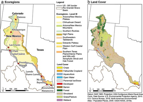
In the U.S., the RGB Socio-Environmental System (SES) as delineated by Koch et al. (2019) encompasses 319,957 km², three states, and nine level III ecoregions (Table 1). The desert ecoregions, Arizona/New Mexico Plateau and Chihuahuan Desert, account for more than half of the SES area. Other ecoregions include semi-arid prairies, i.e. Edwards Plateau, High Plains, and Southwestern Tablelands, a semi-arid plain, i.e. Southern Texas Plains, two mountainous ecoregions, i.e. Arizona/New Mexico Mountains and Southern Rockies, and a sub-tropical ecoregion, i.e. Western Gulf Coastal Plain (U.S. EPA, 2010). In their natural conditions, the sources and timing of streamflow of the basin are highly variable, both spatially and temporally. Upstream of Presidio/Ojinaga, the natural flow regime is primarily driven by snowmelt and peaks in the late spring and early summer (Elias et al., 2015), while in the main tributaries downstream of Presidio/Ojinaga, natural flow regime reaches its maximum level during the monsoon season in late summer to early fall (Ingol-Blanco & McKinney, 2013). The natural flow regimes have been highly disturbed since 1870 due to engineering and water diversions. In the northern reaches of the Rio Grande, the total annual flow is 95% lower than it would have been without human intervention (Blythe & Schmidt, 2018).

Table 1. Spatial extent of the three U.S. States and level III Ecoregions (% of the U.S. RGB)

Area	%
States
Colorado	6
New Mexico	52
Texas	42
Ecoregions
Arizona/New Mexico Mountains	7
Arizona/New Mexico Plateau	11
Chihuahuan Desert	44
Edwards Plateau	5
High Plains	4
Southern Rockies	9
Southwestern Tablelands	13
Southern Texas Plains/Interior Plains and Hills with Xerophytic Shrub and Oak Forest	5
Western Gulf Coastal Plain	2

The distribution of the scarce and over-allocated water resources of the RGB is governed by a complex setup of agreements, regulations, bi-national treaties, inter-state compacts, and physical infrastructures (i.e. dams, levees, diversions, irrigation canals, channelization projects) that operate on multiple scales (Koch et al., 2019; Nava & Sandoval-Solis, 2014). While large-scale development of irrigated agriculture intensified during the 19^th century and especially after the Desert Land Act of 1877, crop irrigation has been essential for the livelihoods of Native peoples in the basin (Blythe & Schmidt, 2018; Scurlock, 1998). Today, agriculture is by far the largest water use, accounting for approximately 85% of surface water and groundwater (estimate based on U.S. Geological Survey (2010)). Moreover, water is also withdrawn for urban and rural domestic use, industry, and hydroelectric power. The river and its tributaries are also a critical freshwater resource for recreational activities (Ortiz-Partida et al., 2016) and provide riparian and aquatic habitats to several endemic and endangered species of the U.S. Southwest (Dettinger et al., 2015; Ruhí et al., 2016).

In 2008, land-use was dominated by shrubland (66%), grassland/pasture (17%), evergreen forest (10%), developed areas (2%) and barren land (1%). Despite the large amount of water used for agriculture, in 2008, agricultural land covered around 915,000 ha in the U.S. portion of the RGB SES, which amounts to only 3% of the basin, of which 201,900 ha were fallow/idle cropland (USDA NASS, 2018a). Croplands are clustered in the floodplains along the Rio Grande and its major tributaries, and in areas with access to groundwater. Major crops produced in the study area in 2008 were sorghum (275,200 ha), alfalfa (156,000 ha), cotton (43,440 ha), winter wheat (26,565 ha), barley (26,070 ha), pecans (25,560 ha), potatoes (22,670 ha), corn (22,370 ha), and sugarcane (17,730 ha). The RGB is a leading producer for several of these crops, including potatoes grown in the San Luis Valley of Colorado (DiNatale Water Consultants, 2015), pecans, onions, chili, and grapes produced in the Middle Rio Grande and Mesilla Valleys in New Mexico (USDA, 2019), and citrus, sugar cane, and vegetables cultivated in the Lower Rio Grande Valley in Texas (Texas A&M AgriLife Research, 2019).

Data

We used the USDA National Agricultural Statistics Service (NASS) Cropland Data Layer (CDL) to study the fallow land and cropland dynamics in the U.S. portion of the RGB SES between 2008 and 2018. The CDL is a satellite-derived, crop-specific land cover dataset. It classifies more than 130 land cover types and provides a detailed classification of crop types including row crops, fruits, and vegetables (USDA NASS, 2018a). A detailed list of all categories and associated codes is available in Supplementary Information Table S1. The CDL also tracks cultivated fallow/idle cropland. According to the USDA Farm Service Agency (FSA), fallow is defined as „unplanted cropland acres which are part of a crop/fallow rotation where cultivated land that is normally planted is purposely kept out of production during a regular growing season„ (USDA FSA, 2020, p. 5).

The CDL is available on a yearly basis starting in 2008 for the contiguous U.S. at a spatial resolution of 30 meters. It was produced from medium resolution satellite imagery (10–60 m) collected throughout the growing season. Over time, different imagery inputs have been used, depending on imagery availability and accessibility. Prior to 2010, the CDL was generated from the Landsat 5 Thematic Mapper (TM) sensor and the Resourcesat-1 (IRS-P6) Advanced Wide Field Sensor (AWiFS). In 2010/2011, the CDL program switched to Landsat-7 Enhanced TM (ETM), and DEIMOS-1 and UK-2 from the Disaster Monitoring Constellation (DMC). More recently, the program has been using the Landsat 8 OLI/TIRS sensor (starting in 2013), the ISRO ResourceSat-2 LISS-3 (starting in 2017), and the ESA Sentinel-2 A and B sensors (starting in 2018) (USDA NASS, 2018a). The NASS leverages other major sources of inputs to produce the CDL. The FSA Common Land Unit (CLU) Program is a national ground truth dataset of USDA farm program crops, collected by NASS County Field Offices. The CLU is split up in two datasets: one is used to train the classifier and distinguish between different crop types, while the other is used for accuracy assessment validation of the cultivated crop classes. NASS generates its own mapping of non-agricultural land cover classes for the CDL based on data from the USGS National Land Cover Dataset (NLCD) released every five years, along with the National Elevation Dataset (NED), percent tree canopy, and percent imperviousness used as ancillary data to separate the non-agricultural areas (Boryan et al., 2011). The CDL also relies on ground truth data from the NASS June Agricultural Survey that served to build a regression model estimate. From this set of data, NASS analysts perform data processing and classification at the state level and mosaic the results in a nationwide CDL map (Lark et al., 2017).

In addition to the CDL, we used the states, ecoregion, and SES (extended basin) boundaries of our study area to perform a multi-scale analysis. We used the following sources: the 2018 version of the U.S. Census cartographic states boundary (U.S. Census Bureau, 2018), the 2006 version of the U.S. EPA Level III ecoregions of the U.S. (U.S. EPA, 2010), and the RGB SES boundary delineated by Koch et al. (2019) (Figure 1). The latter extends the hydrological boundary to include three counties in South-eastern Texas, i.e. Cameron, Hidalgo, and Willacy, where RGB main-stem water is used outside of the hydrological basin boundary. A change in land use in these counties can have a major effect on the stream flow of the Rio Grande, underpinning the need to include land-use dynamics in this area rather than restraining the study to the hydrological basin boundary.

Data processing and analysis

We divided the workflow of the study into two steps (Figure 2): (1) time-series data processing; and (2) analysis of spatial patterns and temporal dynamics by calculating three types of indicators. The following subsections describe each step.

Figure 2. Data processing and analysis workflow

Data collection and processing

We acquired the CDL annual time series for the entire available period when we conducted the study, i.e. 2008–2018, as raster-based GeoTIFF files for the states of Colorado, New Mexico, and Texas from the web application CropScape (Han et al., 2012). We then processed these datasets using ESRI’s ArcGIS (version 10.6) functionalities and the arcpy library. First, we selected the study area extent and generated 11 gridded annual maps of land-use for the RGB SES, preserving the spatial resolution (30 m) and projection (USA Contiguous Albers Equal-Area Conic USGS) of the original datasets. Next, we derived a mask of the total agricultural land (areas that were in cropland or fallow/idle cropland at least once between 2008 and 2018) by performing a binary classification over the 11 gridded annual maps. The pixels classified at least once as fallow/idle cropland [code 61] (henceforth: ‘fallow land’) or cropland [codes 1–60, 66–77, 204–254] (henceforth: ‘cropland’) were included in the mask, and other land cover classes were excluded from the mask. The resulting mask contained more than 18.75 million pixels, or an area of 16,877 km². Next, we constructed a time-series that reports in a tabular format the sequence of land-uses for all pixels contained in the total agricultural land mask. We added the FIPS State Numeric Code, and the Ecoregions Level III Numeric Code of all entries. To determine the codes, we overlaid the time-series data with the states and Level III ecoregion boundaries. The Python processing scripts are available on OSF/GitHub (https://osf.io/c7n3u/).

Data analysis

We calculated three groups of indicators to analyse the spatial patterns and temporal dynamics of fallow land in relation to cropland: (i) the spatial extent of fallow land and cropland, (ii) fallowing and cropping frequencies, and (iii) post-fallow land-use types. To describe the spatial extent of fallow land and cropland, we estimated the area of fallow land and cropland in square kilometres, and the yearly percentage of fallow land and cropland at three scales: RGB level (i.e. for the entire U.S. RGB SES), state level, and ecoregion level. We also estimated the percentage of fallow land for each ecoregion within each state to determine if for ecoregions spanning multiple states, trends were different among jurisdictions.

To assess the fallowing and cropping frequencies, we counted the number of times a pixel was classified as fallow land or cropland over the length of the time-series (11 years). We mapped the frequencies and aggregated the pixel frequencies for the RGB SES.

To determine the major post-fallow land-use categories, we estimated the cumulative area of each land-use following fallow over the entire time-series. We assessed their respective proportion by dividing the cumulative area of each post-fallow land-use category by the total area of fallow. The share of post-fallowing land-use was measured at the RGB SES and state levels.

We used R (version 3.5.3) and ggplot2 package to calculate the indicators and create the plots. We calculated the frequencies and created the maps with arcpy and ESRI’s ArcGIS. The Python and R scripts for calculating the indicators are available on OSF/GitHub (https://osf.io/c7n3u).

Data accuracy

NASS performs an accuracy assessment of the CDL classification each year at the state level. To do so, the CDL maps are compared against independent datasets from the CLU for all cultivated land-cover classes and against the NLCD for non-agricultural land-cover classes (USDA NASS, 2018a). Annual error matrices that report the number of times a particular CDL land-cover class is consistently mapped or not, along with several accuracy statistics, are released and published on the NASS website (USDA NASS, 2018b). The CLU, which is one of the most complete datasets of U.S. agricultural land-cover, provides a robust ground-truth reference dataset for land-cover classification validation. However, it is not publicly available (Johnson, 2013).

Drawing on the annual error matrices and based on the equations proposed by Olofsson et al. (2013), we calculated the stratified error-adjusted areas of cropland, fallow land, and non-agricultural land-uses for the states of Colorado, New Mexico and Texas, with a margin of error at approximately 95% confidence interval (Supplementary Table S2). We could not perform an error adjustment for our study area because we did not have access to location data on the sampling points. Having these locations is necessary to aggregate the data to different ecoregions and states and being able to calculate the stratified error-adjusted area at those levels.

As an alternative to the stratified error-adjusted estimates approach, we derived three area-weighting metrics for our study area: the user’s accuracy, the producer’s accuracy, and the accuracy-derived bias. To do so, we multiplied the CDL state-level user’s accuracy and producer’s accuracy of the class ‘fallow/idle cropland’ by the annual area of that class in each state and for each year (within the boundary of the RGB SES). We added up the results for the three states and divided by the annual area of fallow land for the RGB SES. We then estimated the accuracy-derived bias as negative one plus the ratio of producer’s accuracy and user’s accuracy (Olofsson et al., 2013). The bias evaluates the tendency of a remote sensing product to underestimate or overestimate the area of a land-use category compared to the ground truth data; a negative value corresponds to an underestimation and a positive value to an overestimation. The estimation of the weighted average for the producer’s accuracy (51%) and the bias (−31%) scored poorly (Supplementary Information Table S3). This means that for our study area, the CDL has substantially underestimated the area of fallow/idle cropland across years and states, compared to its reference data. Lark et al. (2017) identified a similar issue for the total cultivated area at the national level, however to a lesser extent.

When using the CDL for land-use change analysis, it is important to be aware that there are three inherent sources of error that can reduce the accuracy of pixel-level change assessments across multiple states (Lark et al., 2015, 2017).

The first source of error is the misclassification of fallow land pixels for two reasons: (1) The fallow/idle cropland category can be confused in source imagery with other land cover categories (e.g. grassland/pasture, barren, shrubland), and (2) mixed pixels often occur along the field boundaries because of a misalignment between fields and pixels. This risk of edge effect can result in inconsistencies of land-use mapping over time and skew the analysis of pixel-based land-cover changes.

The second source of error is due to an improvement of the CDL products. The magnitude of undermapping fallow land has decreased over the years at the RGB SES level and in New Mexico (Supplementary Information Figure S4). This underestimation bias can falsely be interpreted as an increase in fallow land or cropland, and should be considered when interpreting the results. Similarly, the accuracy of our results is dependent on changes in NLCD mapping methodology used to classify non-agricultural land-covers classes in the CDL. This could lead to sudden changes between non-agricultural land-covers categories when NLCD products are released (2011 and 2016 for our study period). This was not considered to be a major issue for the purpose of our study since we did not estimate absolute changes between agricultural land cover and non-agricultural land cover categories in a bi-temporal change analysis, but rather focused on major post-fallow land-use trends and relative importance.

The third source of error is due to state-to-state variations. The USDA NASS independently processes and classifies the annual CDL for each state, which can lead to different interpretations of remotely sensed data, and result in inconsistencies across states. For the fallow/idle cropland category, the area estimation bias differs widely between states (Supplementary Information Figure S4). We found a lower bias for Colorado than for New Mexico and Texas, indicating higher accuracy for Colorado than for the two other states, where fallow areas have been undermapped.

Lark et al. (2017) proposed a set of post-classification processing steps to overcome the pitfalls linked to these sources of errors, including using a minimum unit of change and using a temporal filter. We did not apply these recommendations for the following reasons. Using a minimum unit of change (occurring above 2 ha or even 6 ha) reduces the capacity of our analysis to detect changes occurring in smaller fields (e.g. 1 ha or less), which are prevalent in some sections of the RGB SES, for instance, in the acequias community ditch associations of New Mexico (Rango et al., 2013). Also, the use of a temporal filter is not appropriate for our purpose because it would eliminate all one-year fallowing in the cropping sequence and undermine our capacity to detect cropping rotations with an alternance of several years of crops and one-year fallow, although this is a common farming practice.

Results

Temporal dynamics of fallow and crops

Basin-wide dynamics

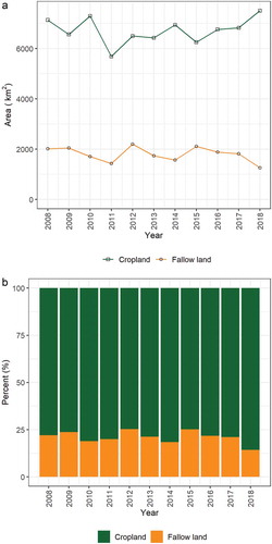
At the basin level, fallow land area and cropland area fluctuated. Since 2012, fallow land area decreased from a maximum area of 2,199 km² to a minimum of 1,256 km² (2018), i.e. a 43% decrease. By contrast, after a substantial drop between 2010 and 2011, cropland area increased from 5,685 km² (2011) to 7,508 km² (2018), i.e. a 16% increase (Figure 3(a)). On average, fallow land area covered 1,800 km² and cropland area around 6,720 km² over the analysed period. The average percentage of fallow land and cropland were about 21% and 79%, respectively. Fallow land ranged from a minimum of 14% (2018) to a maximum of 25% (2012) (Figure 3(b)).

Figure 3. Temporal dynamics of fallow and cropland areas at the basin level between 2008 and 2018. Panel A displays changes in the area of fallow and cropland in km². Panel B displays changes in yearly fallow and cropland percentages

State-level dynamics

The analysis of fallow dynamics at the state level showed a net increase of fallow land area for Colorado and New Mexico and a net decrease for Texas (Figure 4(a)). In New Mexico, the increase was constant, whereas in Colorado, fallow area fluctuated, in particular between 2014 and 2018; area increased from 101 km² (2014) to 321 km² (2017), and then decreased to 167 km² (2018). The proportion of fallow land also differed among states. On average, Colorado had the lowest value (9%), compared to New Mexico and Texas (24% in both states). The overall trends in the U.S. state portions of the RGB SES differed with the spatio-temporal patterns of the whole states. Colorado recorded a higher proportion of fallow land (27% on average) than its RGB SES portion while the proportion of fallow land in Texas (11%) was lower than in its RGB SES portion. New Mexico recorded similar percentages of fallow land (29% on average) compared to its RGB SES portion (Supplementary Figure S5).

Figure 4. Temporal dynamics of fallow and cropland areas at the state level between 2008 and 2018. Panel A displays changes in the area of fallow and cropland in km². Panel B displays changes in yearly fallow and cropland percentages

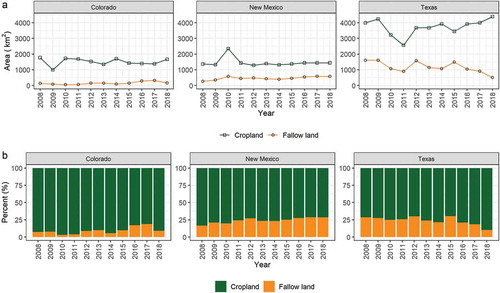
Regarding cropland, New Mexico and Texas recorded a net increase in area while Colorado displayed a net decrease (Figure 4). In New Mexico, with the exception of a peak in 2010, cropland area gradually increased at an average rate of 5% per year. By contrast, the cropland area in Colorado and Texas fluctuated.

While we expected the spatial extent of fallow to increase at the expense of cropland due to the retirement of cropland, overall, fallow dynamics showed no clear relationship with cropland dynamics. For example, we found that the area of fallow and cropland during some periods had a positive relationship (e.g. between 2008 and 2012 in Texas), while other periods showed a negative relationship (e.g. between 2014 and 2018 in Texas). This lack of clear relationship between cropland and fallow dynamics was not restrained to the RGB SES but was also observed for the whole states of Colorado, New Mexico, and Texas (Supplementary Figure S5).

Ecoregion-level dynamics

The analysis of fallow dynamics at the ecoregion level reveals a net decrease of fallow land area for two out of three semi-arid prairies (Edwards Plateau, High Plains), the semi-arid plains (Southern Texas Plains), and one out of two desert ecoregions (Chihuahuan Desert) (Figure 5). Fallow land area increased in the other desert ecoregion (Arizona/New Mexico Plateau), the semi-arid prairie of Southwestern Tablelands, the mountainous ecoregions (Arizona/New Mexico Mountains and Southern Rockies), and the sub-tropical ecoregion of Western Gulf Coastal Plain. Cropland area increased in all ecoregions except in the Arizona/New Mexico Plateau and in the Southwestern Tablelands. For two ecoregions (Southern Texas Plains, Western Gulf Coastal Plain), the variation in cropland area was relatively small (< 5%). As at the state level, the cropland dynamics showed no clear relationship with the fallow dynamics.

Figure 5. Temporal dynamics of fallow and cropland areas at the ecoregion level between 2008 and 2018. Panel A displays changes in the area of fallow and cropland in km². Panel B displays changes in yearly fallow and cropland percentages

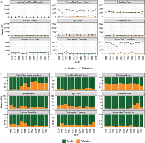
The proportion of fallow land for the Chihuahuan Desert (48%) was twice as high as the RGB SES average (21%). This is the only ecoregion where the proportion of fallow land exceeded the proportion of cropland five years out of 11 (2008, 2012, 2013, 2015, 2016). We found the lowest averages in the Western Gulf Coastal Plain, the Arizona/New Mexico Plateau, and the Southern Rockies (around 8% each).

Ecoregion-level dynamics within the states

We found contrasting fallow land dynamics for the ecoregions in the three states (Supplementary Information Figure S6). In Texas, the Chihuahuan Desert and the High Plains showed a substantial decrease in the proportion of fallow land compared to the four other ecoregions present in the state (Arizona/New Mexico Mountains, Edwards Plateau, Southern Texas Plain, Western Gulf Coastal Plain). Fallow land dynamics displayed interstate variations for several ecoregions. For example, for the Arizona/New Mexico Plateau, the proportion of fallow land in New Mexico was low (less than 3%) and remained stable over time, while it varied between 3% and 19% in Colorado. For the Chihuahuan Desert, fallow land dynamics differed between the states of New Mexico and Texas. The proportion of fallow decreased from 71% (2008) to 34% (2018) in Texas, while the proportion of fallow was increased by 1.5 times in New Mexico.

Fallowing and cropping frequencies

The analysis of frequencies at the RGB SES level revealed distinctly different patterns for fallow and cropland areas. Figure 6 shows that lands with a fallowing frequency equal to one or two years out of 11 – which account for almost 75% of the fallowing frequencies – are more prevalent than lands with a fallowing frequency of nine or more. By contrast, the distribution of cropping frequencies followed a binomial trend. Lands with a cropping frequency equal to one or two represented 36% of the area which is similar to lands with a cropping frequency of nine or more (39%).

Figure 6. Distribution of fallowing and cropping frequencies for the U.S. RGB. Panel A displays the fallowing frequencies and Panel B displays the cropping frequencies. The frequencies represent the number of times that pixels were classified as fallow land or as cropland over the 11-year period. Panel C displays the totals of fallowing and cropping frequencies at the U.S. RGB level

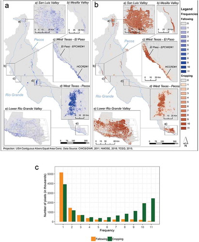
We found a heterogeneous spatial distribution of fallowing and cropping frequencies across the study area. Several hotspots of fallow land (clusters of land with a high density of fallow frequencies above 5) were present; for example, Costilla County in southern Colorado, Chaves and Eddy Counties along the Pecos River in eastern New Mexico, and Culberson and Reeves Counties in West Texas. Main commercial farming areas such as the San Luis Valley, the Mesilla Valley, West Texas, and the Lower Rio Grande Valley, displayed high cropping frequencies and low fallowing frequencies (Figure 6). However, within these farming areas, we observed distinct patterns. For example, the eastern part of the San Luis Valley and the southwestern part of the Lower Rio Grande Valley – along the Mexican border – showed higher fallow frequencies. Similarly, in West Texas, the Hudspeth County Conservation and Reclamation District (HCCR) displayed higher fallowing frequencies than the upstream El Paso County Water Improvement District No. 1 (EPCWID#1).

Post-fallow land-use categories

At the RGB SES level, 45% of the land in fallow over the time period was followed by another year of fallow, while 29% of fallowed land was followed by shrubland and 6% by grassland/pasture (Table 2). The main crops in rotation with fallow included: sorghum (5%), cotton (4%), alfalfa (3%), winter wheat (1%), corn (1%) and potatoes (1%). These crops correspond to the major crops cultivated in the RGB SES (see section 2.1).

Table 2. List of post-fallow land-uses categories ranked in descending order for the period 2008–2018. The proportion is calculated by dividing the cumulative area of each post-fallow land-use category by the total area of fallow land

Land-Use Category	Proportion (%)
Fallow	44.54
Shrubland	28.85
Grassland/Pasture	6.04
Sorghum	4.90
Cotton	3.60
Alfalfa	3.15
Winter Wheat	1.19
Corn	0.98
Potatoes	0.83
Barren	0.73
Other Hay/Alfalfa	0.65
Developed/Open Space	0.65
Barley	0.58
Oats	0.41
Onion	0.33
Sugarcane	0.33
Pecans	0.31
Others	1.91

At the state level, fallow, shrubland, and grassland/pasture were also frequent post-fallow land-use categories. However, we found different successions given that the cropping patterns (types of crops and area) differ among the three states. In Colorado, alfalfa, potatoes, and barley were the three major crops in rotation with fallow, whereas, in New Mexico we found fallow in rotation with alfalfa, winter wheat, and cotton, and in Texas, with sorghum, cotton, and alfalfa (Supplementary Information Table S7 and Figure S8).

Discussion

The objective of this study was to analyse the spatial and temporal patterns of fallow land across the RGB SES in the U.S. Southwest, based on data from the USDA Cropland Data Layer (2008–2018). Here we discuss the key outcomes from our quantitative analysis in the context of key social and environmental dynamics in the basin.

Temporal dynamics of fallow land and cropland

In the context of over-appropriation of water, dry conditions, and increasing competition for water resources, land fallowing is one practice to reduce the amount of water used for irrigation. This study is the first to analyse to what extent this practice has been used across the U.S portion of the RGB SES. In this spatio-temporal analysis, we tested the hypothesis that the fallow extent increased between 2008 and 2018.

At the RGB SES level, we found that fallow rates fluctuated from 2008 (22%) to its maximum in 2012 (25%) and its minimum in 2018 (14%). No increasing trend in fallow extent was observed, rejecting our hypothesis. Additionally, cropland area did not show a clear increasing or decreasing pattern. The cropland rate changed from 42% (2008) to a minimum of 34% (2011) to a maximum of 45% (2018) (Figure 3). Our results differ from previous studies for another drought-stressed region of the U.S. West, the California Central Valley; these studies found an increasing trend in fallow area for the periods 2007–2009 (Christian-Smith et al., 2014) and 2011–2015 (Melton et al., 2015).

One explanation for not observing an increasing trend in fallow area is that, instead of taking land out of production, farmers adopted other strategies to cope with water scarcity. For example, farmers can decrease their use of water by improving the efficiency of irrigation systems (e.g. replacing flood irrigation with drip irrigation), irrigating less, shifting to less water-intensive crops or cultivars and changing crop rotations, adopting new soil management practices that reduce evaporation and increase soil moisture (e.g. new tillage practices), or adjusting the sowing dates (Bodner et al., 2015; Debaeke & Aboudrare, 2004; Running et al., 2019). Farmers also coped with temporary water shortages using buffering mechanisms such as additional groundwater pumping and use of surface water from reservoir storage (Ward, 2014; Williams et al., 2020). For instance, the Mesilla Valley in New Mexico and the San Luis Valley in Colorado are two important farming areas in the basin where groundwater pumping has long been used by farmers to compensate for surface water shortages during periods of drought. In the San Luis Valley, extensive groundwater pumping plus a prolonged drought starting in 2002 led to the emergence of new governance arrangements and programs to recharge the aquifer by 2032 and avoid wells being shut off by the state water regulator (Rio Grande Basin Roundtable, 2015; Koch et al., 2019). Landowners within the Rio Grande Water Conservation District (RGWCD) formed special groundwater subdistricts that developed a water management plan to recharge over 1,200,000 acre-feet of groundwater over a 20-year period. The first subdistrict that became operational in 2009 (Subdistrict#1) has adopted two approaches to reach this goal. In 2012, well users started to pay a fee for every acre-foot of water used. The revenue generated by these fees – combined with the funds from the federal Conservation Reserve Enhancement Program (CREP) – helps compensate farmers who voluntarily engage in fallowing programs. These fallowing programs were complemented by groups of farmers purchasing productive farms and taking them out of production as well as changes in irrigation practices (e.g. stopping the practice of ‘cornering’ plots by using inefficient dragging irrigation to grow on the produce on the corners of irrigated circular plots). Combined with fairly average precipitation rates during the first five years of these initiatives, by 2017, these measures had recovered 350,000 acre-feet of groundwater (Heide, 2018). However, despite widespread recognition of threats to the aquifer and several years of progress towards recharge, a 2018 drought led farmers to resort again to increased groundwater pumping (RGWCD, 2019a), resulting in the one-year extraction of 200,000 acre-feet of the 350,000 that had been recharged over the previous five years.

Another explanation for no increase in fallow area and percentage is that, by limiting the analysis to a recent time period (2008–2018) due to data availability, the study does not capture shifts from cropland to fallow land that occurred before 2008. Farmers exposed to severe droughts prior to 2008 (e.g. during the early 2000’s drought) may have already adapted cropping patterns and permanently retired land, which then was no longer classified as a cropland or fallow/idle cropland in 2008.

We also checked the effect of the fallow/idle cropland underestimation bias as explanation for the magnitude of changes in fallow land area at the RGB SES and state levels, especially in Texas and New Mexico where we observed substantial bias fluctuations (Supplementary Information Figure S4). We found similar trends between uncorrected and bias-adjusted CDL values (Supplementary Information Table S9). This means that the change of class underestimation bias over time cannot explain the overall land fallowing trends at the RGB SES and state-levels.

A last key finding regarding the temporal dynamics is that almost 75% of the area fallowed over the time-period was in fallow only once or twice (Figure 6), showing that fallowing was primarily a temporary practice.

Spatial heterogeneity across the basin

Multi-scale analyses across large areas are important to identify regional land-use transitions under diverse social and environmental conditions (Corbelle-Rico et al., 2012). Hence, our second hypothesis was that land fallowing is more prominent in the desert ecoregions of the basin.

First, our results show that fallow patterns varied widely across ecoregions without a clear, distinctive trend (Figure 5). One ecoregion stood out, however.In the Chihuahuan Desert, the percentage of fallow land was always higher than in any other ecoregion and, even if it decreased over time, was on average twice as high as the RGB SES average. Furthermore, this was the only ecoregion where fallow area exceeded cropland area for five years out of 11. These results are in contrast with the other desert ecoregion (the Arizona/New Mexico Plateau) where contrary to our expectations, the percentage of fallow land was lower than the RGB SES average.

Second, we found differences in fallowing practices among the states that were not visible in the RGB SES-level analysis. Fallow land area decreased in Texas, increased in New Mexico, and did not show a clear trend in Colorado. Furthermore, Colorado had the lowest proportion of fallow land of the three states. Despite the presence of fallowing programs in the San Luis Valley (Colorado) since 2012, the state-level analysis neither captured an increase in fallowing area nor a higher percentage of fallow land. The state-level analysis covers a much larger area than the San Luis Valley which can explain why we do not capture such dynamic. However, annual reports from Subdistrict #1 of the San Luis Valley show that while economic incentives are available to fallow up to 160 km² in the district, only 35 km² have been enrolled under the fallowing program in 2018 (RGWCD, 2013, 2014, 2015, 2016, 2017, 2018, 2019b) (Supplementary Information Table S10). The area fallowed under the lease-fallowing program has increased over time, but the program still remains underused. This suggests the existence of barriers for farmers to engage in the program. More research is needed to understand the drivers that influence the different patterns across states but also the factors hindering the adoption of such funded conservation practices.

Another result was the identification of distinct trends for the state portions of the RGB SES compared to the states' overall trends. The fact that the Colorado portion of the RGB SES has a lower proportion of fallow land than the state average confirms that agriculture is intensive in this section of the RGB and compared to the rest of the state. By contrast, the Texas portion of the RGB recorded a higher rate of fallow land in rotation with crops than the state average. Except for the Lower Rio Grande Valley along the Gulf of Mexico, a large amount of the agricultural land of the RGB SES in Texas is found in semi-arid areas at the west of the 100^th Meridian, with restricted access to surface or groundwater irrigation, which limits the potential for crop cultivation, compared to more rainy regions in the east of the state.

A last key finding from our study was the identification of several hotspots of fallowing , for example, in south-eastern Colorado, along the Pecos river, in West Texas, and south of El Paso in the Hudspeth County Conservation and Reclamation District #1 (HCCRD#1). In contrast, irrigation-intensive areas such as the San Luis Valley (CO), Hatch and Mesilla Valleys (NM), El Paso County Water Improvement District No. 1 (EPCWID#1), and the Lower Rio Grande Valley (TX) have low fallowing frequencies (Figure 6). The fact that two neighbouring irrigation districts, EPCWID#1 and HCCRD#1, located in the same state (TX) and ecoregion (Chihuahuan Desert), have diverging patterns shows that regional environmental conditions and state water management plans cannot solely explain the spatio-temporal fallowing dynamics. A combination of local drivers also influences these patterns. In this case, drivers include increased soil and water salinity, decreased streamflows in the river system, and differences in access to surface water. In fact, farmers in EPCWID#1 have legal rights to Rio Grande surface water stored in the upstream Elephant Butte and Caballo reservoirs (via the Rio Grande Project), whereas farmers in the adjacent HCCRD#1 only rely on excess flows and irrigation returns that pass downstream from EPCWID#1 (Hogan, 2013).

Limitations and next steps

Our approach includes several limitations. We chose the CDL dataset, since this is the longest time-series and the best crop-specific land cover satellite-derived dataset available at a 30 m resolution for the contiguous U.S. (Johnson, 2013; Wright & Wimberly, 2013). As a result, its use has been growing steadily, for example, to track land-use and land-cover change (Lark et al., 2015; Wright et al., 2017; Wright & Wimberly, 2013), to derive maps of tilled cropland (Johnson, 2013), to assess the impact of landscape-scale agricultural diversity on U.S. crop production (Burchfield et al., 2019), and to quantify the determinants of land-cover change (Stoebner & Lant, 2014). However, tracking fallow land area dynamics with the CDL poses several challenges. As recommended by Lark et al. (2017), we characterized the bias but, instead of limiting our study to a bi-temporal change analysis, we quantified fallow dynamics over the entire time-series for comparisons across states and years. Our results have shown that almost 75% of the area fallowed over the time-period was in fallow once or twice, but this could also be the result of CDL misclassifications. 36% of the area in fallow was followed by shrubland, grassland/pasture, barren, or developed/open space land (Table 2). Instead of an actual change in land cover, this could be the effect of classifier confusion, which is notoriously hard to differentiate (Johnson, 2013; Lark et al., 2017). However, to date, the CDL is the best and longest crop-specific land-cover dataset available for the U.S. To remove potential misclassification errors, previous studies (e.g. Lark et al. (2015)) applied post-processing methods such as temporal filters and minimum mapping units. We chose to not follow this method because this would have undermined our capacity to detect one-year fallowing as well as fallowing occurring in small areas. Furthermore, we did not restrain our analysis to the pixels that were always in fallow or cropland from 2008 to 2018, because we would have not been able to account for the gains or losses of cropland areas. Another limitation when using the CDL is its ability to accurately map areas that are managed as fallow. Depending on the biophysical and especially climatic conditions and farmers’ management, fallow areas range from remaining free of vegetation to weedy or shrubby vegetation cover (Johnson, 2013; Wallace et al., 2017), making the classification more challenging. However, as we show above, the fallow/idle cropland classification has improved over time.

For our study area, the CDL is only available for the years 2008 to 2018. Analysing a longer time period (at least 30 to 50 years) would help us to understand if the fallowing dynamics are recurrent fluctuations, i.e. as part of a traditional crop-fallow rotation practice, or long-term trends motivated by climate change and/or other socio-environmental changes. A potential way to analyse a longer time period is a multi-temporal analysis of remote-sensing image data (de Beurs & Ioffe, 2013; Yin et al., 2018). Comparing fallowing patterns between several known extended periods of droughts and wet periods would also help to understand if the fallowing dynamics are episodic patterns related to drought and wet times. However, establishing such correlation in future research raises a certain number of methodological challenges. For example, farmers’ responses to drought may be delayed, especially if they use buffer mechanisms (access to groundwater and reservoir storage).

We limited our analysis to describing and quantifying the spatio-temporal patterns of fallowing, which does not allow us to draw conclusions about the causes of the variations observed. Future research should aim to connect these patterns to the outcomes of research focused on water management to understand the underlying drivers of fallowing decisions across the basin. Beyond drought, many factors may contribute to land-use/land-cover change (Mottet et al., 2006; van Vliet et al., 2015), including biophysical (e.g. soil quality, topography, accessibility), economic (e.g. prices, consumers demand, markets), technological (e.g. improvement of water use efficiency, farm intensification), sociodemographic and cultural (e.g. farm succession, farmers’ age), political (e.g. international trade agreements, subsidies, water policies), and agronomic factors (e.g. soil fertility restoration, plant disease management). A better understanding of the role of such factors will help to better target and enhance the effectiveness of water conservation policies.

Conclusion

In the U.S. Southwest, chronic water-scarcity and increasing non-irrigation water demands put a strain on irrigated agriculture. Land fallowing is one of the potential responses for coping with reduced water availability. Through a multi-scale analysis of the USDA Cropland Data Layer (2008–2018), we studied the spatial and temporal patterns of fallow lands and croplands across the U.S. portion of the Rio Grande/Río Bravo Socio-Environmental System (RGB SES) to identify where land fallowing is taking place, to what extent, and with what frequency. Against our hypothesis that land fallowing has been increasing in the RGB SES, the results did not reveal any clear increasing or decreasing trend of fallow land at the SES level. We found heterogeneous dynamics across states and ecoregions, and detected hotspots of fallowing, especially in West Texas. The Chihuahuan desert stood out in our study: the area of fallow exceeded the area in cropland five years out of 11 and the percentage of fallow lands was higher than in other ecoregions of the basin. These findings demonstrate the importance of multi-scale analyses in a large spatial area to better understand land-use strategies across distinct social and ecological contexts. Tracking the spatial location and historical dynamics of fallow and cropland is important for informing changes in farming practices, their adaptability to water supply conditions, and, ultimately, their impacts on water resources, since changes in land-use patterns have direct effects on water consumption levels, evapotranspiration, and run-off. These results also illustrate that fallowing is still an underused mechanism for reducing water use at a larger scale. As climate change and new non-agricultural demands increase stress on water supply for irrigation, this type of information is critical to monitor water conservation efforts and support water managers and policy makers in the design of sustainable water resource and land management plans. Further research should prioritize the study of fallowing hotspots and investigate the driving factors, especially climatic and socio-economic factors, on the spatio-temporal dynamics of land use in the RGB.

Disclosure of potential conflicts of interest

No potential conflict of interest was reported by the author(s).

Acknowledgments

We would like to thank Dr. Kirsten de Beurs for providing guidance on data accuracy assessment and the two anonymous reviewers for their helpful comments and suggestions.

Supplemental data

Supplemental data for this article can be accessed here.

Additional information

Funding

The project described in this publication was supported by Grant No. G15AP00132 from the U.S. Geological Survey. Its contents are solely the responsibility of the authors and do not necessarily represent the views of the South-Central Climate Adaptation Science Center or the U.S. Geological Survey. This manuscript is submitted for publication with the understanding that the U.S. Government is authorized to reproduce and distribute reprints for Governmental purposes;U.S. Geological Survey [G15AP00132];

References

- Bangsund, D.A., Hodur, N.M., & Leistritz, F.L. (2004). Agricultural and recreational impacts of the conservation reserve program in rural North Dakota, USA. Journal of Environmental Management, 71(4), 293–303. https://doi.org/10.1016/j.jenvman.2003.12.017
- Blythe, T.L., & Schmidt, J.C. (2018). Estimating the natural flow regime of rivers with long-standing development: The Northern Branch of the Rio Grande. Water Resources Research, 54(2), 1212–1236. https://doi.org/10.1002/2017WR021919
- Bodner, G., Nakhforoosh, A., & Kaul, H.-P. (2015). Management of crop water under drought: A review. Agronomy for Sustainable Development, 35(2), 401–442. https://doi.org/10.1007/s13593-015-0283-4
- Booker, J.F., Michelsen, A.M., & Ward, F.A. (2005). Economic impact of alternative policy responses to prolonged and severe drought in the Rio Grande Basin. Water Resources Research, 41(2), W02026. https://doi.org/10.1029/2004wr003486
- Boryan, C., Yang, Z., Mueller, R., & Craig, M. (2011). Monitoring US agriculture: The US Department of Agriculture, National Agricultural Statistics Service, Cropland Data Layer Program. Geocarto International, 26(5), 341–358. https://doi.org/10.1080/10106049.2011.562309
- Burchfield, E.K., Nelson, K.S., & Spangler, K. (2019). The impact of agricultural landscape diversification on U.S. crop production. Agriculture, Ecosystems & Environment, 285, 106615. https://doi.org/10.1016/j.agee.2019.106615
- Cayan, D.R., Das, T., Pierce, D.W., Barnett, T.P., Tyree, M., & Gershunov, A. (2010). Future dryness in the southwest US and the hydrology of the early 21st century drought. Proceedings of the National Academy of Sciences, 107( 50), 21271–21276. https://doi.org/10.1073/pnas.0912391107
- Chavarria, S.B., & Gutzler, D.S. (2018). Observed changes in climate and streamflow in the Upper Rio Grande Basin. JAWRA Journal of the American Water Resources Association, 54(3), 644–659. https://doi.org/10.1111/1752-1688.12640
- Chemura, A., Rwasoka, D., Mutanga, O., Dube, T., & Mushore, T. (2020). The impact of land-use/land cover changes on water balance of the heterogeneous Buzi sub-catchment, Zimbabwe. Remote Sensing Applications: Society and Environment, 18, 100292. https://doi.org/10.1016/j.rsase.2020.100292
- Christian-Smith, J., Levy, M.C., & Gleick, P.H. (2014). Maladaptation to drought: A case report from California, USA. Sustainability Science, 10(3), 491–501. https://doi.org/10.1007/s11625-014-0269-1
- Corbelle-Rico, E., Crecente-Maseda, R., & Santé-Riveira, I. (2012). Multi-scale assessment and spatial modelling of agricultural land abandonment in a European peripheral region: Galicia (Spain), 1956–2004. Land Use Policy, 29(3), 493–501. https://doi.org/10.1016/j.landusepol.2011.08.008
- CWCB. (2018). Colorado Drought Mitigation and Response Plan. https://drought.unl.edu/archive/plans/Drought/state/CO_2018.pdf
- de Beurs, K.M., & Ioffe, G. (2013). Use of Landsat and MODIS data to remotely estimate Russia’s sown area. Journal of Land Use Science, 9(4), 377–401. https://doi.org/10.1080/1747423x.2013.798038
- Debaeke, P., & Aboudrare, A. (2004). Adaptation of crop management to water-limited environments. European Journal of Agronomy, 21(4), 433–446. https://doi.org/10.1016/j.eja.2004.07.006
- Dettinger, M., Udall, B., & Georgakakos, A. (2015). Western water and climate change. Ecological Applications, 25(8), 2069–2093. https://doi.org/10.1890/15-0938.1
- Rio Grande Basin Roundtable. (2015). Rio Grande Basin Implementation Plan. https://www.colorado.gov/pacific/sites/default/files/rgbip-for%20web%20viewing.pdf
- Elias, E.H., Rango, A., Steele, C.M., Mejia, J.F., & Smith, R. (2015). Assessing climate change impacts on water availability of snowmelt-dominated basins of the Upper Rio Grande basin. Journal of Hydrology: Regional Studies, 3, 525–546. https://doi.org/10.1016/j.ejrh.2015.04.004
- Evans, R.G., & Sadler, E.J. (2008). Methods and technologies to improve efficiency of water use. Water Resources Research, 44(7), W00E04. https://doi.org/10.1029/2007WR006200
- FAO. (2014). AQUASTAT - FAO’s Global information system on water and agriculture. Food and Agriculture Organization of the United Nations: Roma, Italy. http://www.fao.org/aquastat/en/
- FAO. (2017). Land use, irrigation and agricultural practices - Definitions. Food and Agriculture Organization of the United Nations: Roma, Italy. http://www.fao.org/economic/ess/ess-home/ua
- Gober, P., & Kirkwood, C.W. (2010). Vulnerability assessment of climate-induced water shortage in Phoenix. Proceedings of the National Academy of Sciences, 107( 50), 21295–21299. https://doi.org/10.1073/pnas.0911113107
- Han, W., Yang, Z., Di, L., & Mueller, R. (2012). CropScape: A Web service based application for exploring and disseminating US conterminous geospatial cropland data products for decision support. Computers and Electronics in Agriculture, 84, 111–123. https://doi.org/10.1016/j.compag.2012.03.005
- Heide, R., (2018). “Tale of Two Rivers” — Happy ending? Alamosa Valley Courrier. September 19, 2018. https://alamosanews.com/article/tale-of-two-rivers-happy-ending
- Hoekstra, A.Y., Mekonnen, M.M., Chapagain, A.K., Mathews, R.E., & Richter, B.D. (2012). Global Monthly Water cSarcity: Blue Water Footprints versus Blue Water Availability. PLoS One, 7(2), e32688. https://doi.org/10.1371/journal.pone.0032688
- Hoekstra, A.Y., & Wiedmann, T.O. (2014). Humanity’s unsustainable environmental footprint. Science, 344(6188), 1114. https://doi.org/10.1126/science.1248365
- Hogan, J.F. (2013). Water quantity and quality challenges from Elephant Butte to Amistad. Ecosphere, 4(1), 9. https://doi.org/10.1890/ES12-00302.1
- Ingol-Blanco, E., & McKinney, D.C. (2013). Development of a Hydrological Model for the Rio Conchos Basin. Journal of Hydrologic Engineering, 18(3), 340–351. https://doi.org/10.1061/(ASCE)HE.1943-5584.0000607
- Johnson, D.M. (2013). A 2010 map estimate of annually tilled cropland within the conterminous United States. Agricultural Systems, 114, 95–105. https://doi.org/10.1016/j.agsy.2012.08.004
- Jones, S.M., & Gutzler, D.S. (2016). Spatial and Seasonal Variations in Aridification across Southwest North America. Journal of Climate, 29(12), 4637–4649. https://doi.org/10.1175/JCLI-D-14-00852.1
- Keshavarz, M., Karami, E., & Vanclay, F. (2013). The social experience of drought in rural Iran. Land Use Policy, 30(1), 120–129. https://doi.org/10.1016/j.landusepol.2012.03.003
- Koch, J., Friedman, J.R., Paladino, S., Plassin, S., & Spencer, K. (2019). Conceptual modeling for improved understanding of the Rio Grande/Río Bravo socio-environmental system. Socio-Environmental Systems Modelling, 1, 16127. https://doi.org/10.18174/sesmo.2019a16127
- Lark, T.J., Meghan Salmon, J., & Gibbs, H.K. (2015). Cropland expansion outpaces agricultural and biofuel policies in the United States. Environmental Research Letters, 10(4), 044003. https://doi.org/10.1088/1748-9326/10/4/044003
- Lark, T.J., Mueller, R.M., Johnson, D.M., & Gibbs, H.K. (2017). Measuring land-use and land-cover change using the U.S. department of agriculture’s cropland data layer: Cautions and recommendations. International Journal of Applied Earth Observation and Geoinformation, 62, 224–235. https://doi.org/10.1016/j.jag.2017.06.007
- Lund, J., Medellin-Azuara, J., Durand, J., & Stone, K. (2018). Lessons from California’s 2012–2016 Drought. Journal of Water Resources Planning and Management, 144(10), 04018067. https://doi.org/10.1061/(ASCE)WR.1943-5452.0000984
- MacDonald, G.M. (2010). Water, climate change, and sustainability in the southwest. Proceedings of the National Academy of Sciences, 107( 50), 21256–21262. https://doi.org/10.1073/pnas.0909651107
- Mekonnen, M.M., & Hoekstra, A.Y. (2016). Four billion people facing severe water scarcity. Science Advances, 2(2), e1500323. https://doi.org/10.1126/sciadv.1500323
- Melton, F., Rosevelt, C., Guzman, A., Johnson, L., Zaragoza, I., Verdin, J., Thenkabail, P., Wallace, C., Mueller, R., Willis, P., & Jones, J. (2015). Fallowed area mapping for drought impact reporting: 2015 assessment of conditions in the California Central Valley. NASA Ames Research Center: Mountain View, CA, USA. https://nex.nasa.gov/nex/static/media/dataset/Central_Valley_Fallowing_Data_Report_14Oct2015.pdf
- Michael, J., Howitt, R., Medellín-Azuara, J., & MacEwan, D. (2010). A retrospective estimate of the economic impacts of reduced water supplies to the San Joaquin Valley in 2009. Business Forecasting Center, University of the Pacific: Stockton, CA, USA. https://www.forecast.pacific.edu/Documents/school-business/BFC/SJV_Rev_Jobs_2009_092810.pdf
- Mote, P.W., Li, S., Lettenmaier, D.P., Xiao, M., & Engel, R. (2018). Dramatic declines in snowpack in the western US. Npj Climate and Atmospheric Science, 1(1), 2. https://doi.org/10.1038/s41612-018-0012-1
- Mottet, A., Ladet, S., Coqué, N., & Gibon, A. (2006). Agricultural land-use change and its drivers in mountain landscapes: A case study in the Pyrenees. Agriculture, Ecosystems & Environment, 114(2–4), 296–310. https://doi.org/10.1016/j.agee.2005.11.017
- Nakat, A.C., & Turner, C.D. (2004). Water use and transfer scenarios in El Paso County, Texas, USA. Water International, 29(3), 338–351. https://doi.org/10.1080/02508060408691788
- Nava, L.F., & Sandoval-Solis, S. (2014). Multi-tiered Governance of the Rio Grande/Bravo Basin: The Fragmented Water Resources Management Model of the United States and Mexico. International Journal of Water Governance, 2(1), 85–106. https://doi.org/10.7564/13-IJWG23
- NMOSE, & NMWRRI. (2018). New Mexico Drought Plan: 2018. https://drought.unl.edu/archive/plans/Drought/state/NM_2018.pdf
- Olofsson, P., Foody, G.M., Stehman, S.V., & Woodcock, C.E. (2013). Making better use of accuracy data in land change studies: Estimating accuracy and area and quantifying uncertainty using stratified estimation. Remote Sensing of Environment, 129, 122–131. https://doi.org/10.1016/j.rse.2012.10.031
- Ortiz-Partida, J.P., Lane, B.A., & Sandoval-Solis, S. (2016). Economic effects of a reservoir re-operation policy in the Rio Grande/Bravo for integrated human and environmental water management. Journal of Hydrology: Regional Studies, 8, 130–144. https://doi.org/10.1016/j.ejrh.2016.08.004
- Pierce, D.W., Barnett, T.P., Hidalgo, H.G., Das, T., Bonfils, C., Santer, B.D., Bala, G., Dettinger, M.D., Cayan, D.R., Mirin, A., Wood, A.W., & Nozawa, T. (2008). Attribution of Declining Western U.S. Snowpack to Human Effects. Journal of Climate, 21(23), 6425–6444. https://doi.org/10.1175/2008JCLI2405.1
- Rango, A., Fernald, A., Steele, C., Hurd, B., & Ochoa, C. (2013). Acequias and the Effects of Climate Change. Journal of Contemporary Water Research & Education, 151(1), 84–94. https://doi.org/10.1111/j.1936-704X.2013.03154.x
- RGWCD. (2013). Special Improvement District #1 of the Rio Grande Water Conservation District. Annual Report for the 2012 Plan Year. https://rgwcd.org/annual-report
- RGWCD. (2014). Special Improvement District #1 of the Rio Grande Water Conservation District. Annual Report for the 2013 Plan Year. https://rgwcd.org/annual-report
- RGWCD. (2015). Special Improvement District #1 of the Rio Grande Water Conservation District. Annual Report for the 2014 Plan Year. https://rgwcd.org/annual-report
- RGWCD. (2016). Special Improvement District #1 of the Rio Grande Water Conservation District. Annual Report for the 2015 Plan Year. https://rgwcd.org/annual-report
- RGWCD. (2017). Special Improvement District #1 of the Rio Grande Water Conservation District. Annual Report for the 2016 Plan Year. https://rgwcd.org/annual-report
- RGWCD. (2018). Special Improvement District #1 of the Rio Grande Water Conservation District. Annual Report for the 2017 Plan Year. https://rgwcd.org/annual-report
- RGWCD. (2019a). Change in unconfined aquifer storage. Year 2002–2019. Retrieved October 15, 2019, from https://rgwcd.org/well-information
- RGWCD. (2019b). Special Improvement District #1 of the Rio Grande Water Conservation District. Annual Report for the 2018 Plan Year. https://rgwcd.org/annual-report
- Richter, B.D., Bartak, D., Caldwell, P., Davis, K.F., Debaere, P., Hoekstra, A.Y., Li, T., Marston, L., McManamay, R., Mekonnen, M.M., Ruddell, B.L., Rushforth, R.R., & Troy, T.J. (2020). Water scarcity and fish imperilment driven by beef production. Nature Sustainability, 3(4), 319–328. https://doi.org/10.1038/s41893-020-0483-z
- Richter, B.D., Brown, J.D., DiBenedetto, R., Gorsky, A., Keenan, E., Madray, C., Morris, M., Rowell, D., & Ryu, S. (2017). Opportunities for saving and reallocating agricultural water to alleviate water scarcity. Water Policy, 19(5), 886–907. https://doi.org/10.2166/wp.2017.143
- Robertson, W.M., Böhlke, J.K., & Sharp, J.M. (2017). Response of deep groundwater to land use change in desert basins of the Trans-Pecos region, Texas, USA: Effects on infiltration, recharge, and nitrogen fluxes. Hydrological Processes, 31(13), 2349–2364. https://doi.org/10.1002/hyp.11178
- Rosegrant, M.W., & Ringler, C. (2000). Impact on food security and rural development of transferring water out of agriculture. Water Policy, 1(6), 567–586. https://doi.org/10.1016/S1366-7017(99)00018-5
- Rosegrant, M.W., Ringler, C., & Zhu, T. (2009). Water for Agriculture: Maintaining Food Security under Growing Scarcity. Annual Review of Environment and Resources, 34(1), 205–222. https://doi.org/10.1146/annurev.environ.030308.090351
- Ruhí, A., Olden, J.D., & Sabo, J.L. (2016). Declining streamflow induces collapse and replacement of native fish in the American Southwest. Frontiers in Ecology and the Environment, 14(9), 465–472. https://doi.org/10.1002/fee.1424
- Running, K., Burnham, M., Wardropper, C.B., Ma, Z., Hawes, J.K., & du Bray, M.V. (2019). Farmer adaptation to reduced groundwater availability. Environmental Research Letters, 14(11), 115010. https://doi.org/10.1088/1748-9326/ab4ccc
- Scurlock, D. (1998). From the Rio to the Sierra: An Environmental History of the Middle Rio Grande Basin ( Report No. RMRS-GTR-5). U.S. Department of Agriculture, Forest Service, Rocky Mountain Research Station.
- Seager, R., Ting, M., Li, C., Naik, N., Cook, B., Nakamura, J., & Liu, H. (2013). Projections of declining surface-water availability for the southwestern United States. Nature Climate Change, 3(5), 482–486. https://doi.org/10.1038/nclimate1787
- Smit, B., & Skinner, M.W. (2002). Adaptation options in agriculture to climate change: A typology. Mitigation and Adaptation Strategies for Global Change, 7(1), 85–114. https://doi.org/10.1023/A:1015862228270
- Stoebner, T.J., & Lant, C.L. (2014). Geographic determinants of rural land covers and the agricultural margin in the Central United States. Applied Geography, 55, 138–154. https://doi.org/10.1016/j.apgeog.2014.09.008
- Texas A&M AgriLife Research. (2019). Lower Rio Grande Valley. Retrieved November 7, 2019, from https://agriliferesearch.tamu.edu/region/lower-rio-grande-valley
- Tressler, A. (2018a, November 26). Alternative methods to success: New ATMs seem as solutions to Colorado’s buy-and-dry problem. The University of Denver Water Law Review. http://duwaterlawreview.com/alternative-methods-to-success-new-atms-seen-as-solutions-to-colorados-buy-and-dry-proble
- Tressler, A. (2018b, May 8). Colorado HB17–1219: Extend CWCB fallowing and leasing pilot program. The University of Denver Water Law Review. http://duwaterlawreview.com/colorado-hb17-1219-extend-cwcb-fallowing-leasing-pilot-program
- TWDB. (2017). 2017 State Water Plan. https://www.twdb.texas.gov/waterplanning/swp/2017/doc/SWP17-Water-for-Texas.pdf?d=7692.440000013448
- U.S. Census Bureau. (2018). 2018 TIGER/Line® Shapefiles. https://www.census.gov/cgi-bin/geo/shapefiles/index.php
- U.S. EPA. (2010). Level III ecoregions of North America. https://www.epa.gov/eco-research/ecoregions-north-america
- U.S. Geological Survey. (2010). Estimated use of water in the United States. County-Level Data for 2010: National Water Information System (NWIS). https://water.usgs.gov/watuse/data/2010/index.html
- UNEP, & Oregon State University. (2002). Atlas of international freshwater agreements (Vol. 4). United Nations Environmental Programme Press: Nairobi, Kenya.
- USDA. (2019). 2017 Census of Agriculture New Mexico. State and County Data ( Report No. AC-17-A-31).
- USDA FSA. (2020). FSA handbook. 2-CP (Rev. 16) acreage and compliance determinations. U.S. Department of Agriculture. Farm Service Agency. https://www.fsa.usda.gov/programs-and-services/laws-and-regulations/handbooks/index
- USDA NASS. (2018a). USDA national agricultural statistics service cropland data layer. https://nassgeodata.gmu.edu/CropScape
- USDA NASS. (2018b). USDA national agricultural statistics service Cropland Data Layer accuracy assessment. https://www.nass.usda.gov/Research_and_Science/Cropland/SARS1a.php
- van Vliet, J., de Groot, H.L.F., Rietveld, P., & Verburg, P.H. (2015). Manifestations and underlying drivers of agricultural land use change in Europe. Landscape and Urban Planning, 133, 24–36. https://doi.org/10.1016/j.landurbplan.2014.09.001
- Vörösmarty, C.J., Green, P., Salisbury, J., & Lammers, R.B. (2000). Global Water Resources: Vulnerability from Climate Change and Population Growth. Science, 289(5477), 284. https://doi.org/10.1126/science.289.5477.284
- Wallace, C.S.A., Thenkabail, P., Rodriguez, J.R., & Brown, M.K. (2017). Fallow-land Algorithm based on Neighborhood and Temporal Anomalies (FANTA) to map planted versus fallowed croplands using MODIS data to assist in drought studies leading to water and food security assessments. GIScience & Remote Sensing, 54(2), 258–282. https://doi.org/10.1080/15481603.2017.1290913
- Ward, F.A. (2014). Economic impacts on irrigated agriculture of water conservation programs in drought. Journal of Hydrology, 508, 114–127. https://doi.org/10.1016/j.jhydrol.2013.10.024
- Weatherhead, E.K., & Howden, N.J.K. (2009). The relationship between land use and surface water resources in the UK. Land Use Policy, 26, S243–S250. https://doi.org/10.1016/j.landusepol.2009.08.007
- Williams, A.P., Cook, E.R., Smerdon, J.E., Cook, B.I., Abatzoglou, J.T., Bolles, K., Baek, S.H., Badger, A.M., & Livneh, B. (2020). Large contribution from anthropogenic warming to an emerging North American megadrought. Science, 368(6488), 314–318. https://doi.org/10.1126/science.aaz9600
- Wong, C.M., Pittock, J., & Schelle, P. (2007). World’ s Top 10 rivers at risk. WWF International: Gland, Switzerland. https://wwfint.awsassets.panda.org/downloads/worldstop10riversatriskfinalmarch13_1.pdf
- Wright, C.K., Larson, B., Lark, T.J., & Gibbs, H.K. (2017). Recent grassland losses are concentrated around U.S. ethanol refineries. Environmental Research Letters, 12(4), 044001. https://doi.org/10.1088/1748-9326/aa6446
- Wright, C.K., & Wimberly, M.C. (2013). Recent land use change in the Western Corn Belt threatens grasslands and wetlands. Proceedings of the National Academy of Sciences, 110( 10), 4134–4139. https://doi.org/10.1073/pnas.1215404110
- Yin, H., Prishchepov, A.V., Kuemmerle, T., Bleyhl, B., Buchner, J., & Radeloff, V.C. (2018). Mapping agricultural land abandonment from spatial and temporal segmentation of Landsat time series. Remote Sensing of Environment, 210, 12–24. https://doi.org/10.1016/j.rse.2018.02.050