Using microworlds for policymaking in the context of resilient farming systems

ABSTRACT

Resilience management of farming systems requires building an understanding of the underlying drivers of the adaptive capacity of the system. In this paper, we use the concept of resilience as a framework to understand how bovine livestock farming systems may adjust to challenging environmental, social, and political conditions. Using an interactive simulation model (microworld), we explored potential developments for livestock farmers in Bourbonnais, France, to the effect of simultaneous changes in the socioeconomic landscape and unpredictable weather conditions resulting from climate change. The results offer insights into the potential trade-offs between systems scale and long-term sustainability by suggesting that sacrificing socioeconomic performance in the short and medium term may increase long-term sustainability and resilience.

KEYWORDS:

• Resilience
• livestock
• dynamic systems
• food systems
• climate change

1. Introduction

In recent decades, European food systems have become more intensive, efficient, and specialised (EEA/European Environment Agency, 2010; European Commission, 2011). These changes have not happened in isolation but as a response to global and regional changes that have increased the size of European markets and opened a world of possibilities and new technologies (Knickel et al., 2018; Saifi & Drake, 2008). However, these gains have come at the expense of a reduction in system resilience, as regional food systems have increased their path dependency and, intentionally or unintentionally, reduced their buffers (Knickel et al., 2018). This lack of resilience was evident in 2018, when multiple farm systems failed to cope with abrupt changes in weather conditions (Beitnes et al., 2022; Beillouin et al., 2020).

Climate change is one of the greatest challenges that farmers have faced in generations (Blanco et al., 2017). Changes in rain patterns, heat waves, and droughts resulting from climate change are already pushing farmers to their limits, and these effects are likely to intensify in the upcoming years (Mitter et al., 2019). As the public becomes more aware of climate change, its effects are leading to cultural, economic, and behavioural changes. An early example of this widespread effect of climate change is the increasing shift in consumer preferences towards more sustainable diets (Hartmann & Siegrist, 2017; Sanchez-Sabate & Sabaté, 2019) and more aggressive policies and regulations limiting the usage of chemical fertilisers (Dubois et al., 2019).

Changes in consumer diets are a concern to those who socially or economically depend on livestock farming systems, particularly those participating in dairy and bovine meat production. Livestock farming systems are a major economic activity in Europe (Olesen & Bindi, 2002), and meat production has experienced steady growth since the end of the second world war (Masters et al., 2016). However, consumption of meat per capita has stagnated in many European countries in recent decades and in some cases have even started to decline (de Boer & Aiking, 2018; Soler & Thomas, 2020). While this decline thus far seems moderate, consumption habits are changing rapidly and raise concerns about a sustainable future for these systems (Mitter et al., 2019; Paas et al., 2021).

While there is little doubt of the impact livestock farming (particularly of bovine cattle) has on climate change, it is important to recognise the impact that losing these farming systems will have in the wider socioecological system. While meat and milk remain part of diets, local livestock systems are still necessary to reduce CO2 emissions. Locally produced food is fundamental to mitigate climate change effects by satisfying food demand with a lower carbon footprint (Pinto-Correia et al., 2021; Schmitt et al., 2017). While meat and dairy remain part of European diets, the extinction of farming systems in the region will increase global CO2 emissions because retailers will have to transport food from elsewhere (Allen et al., 2018). Moreover, this food will need to be packaged and processed, thereby increasing the emissions generated per ton of food produced even more.

Farming systems in Europe are also important for cultural and economic reasons, particularly in rural areas where farming has been the main economic activity for generations and farming systems are part of the local identity and landscape (Moreno et al., 2018; Assandri et al., 2018). The extension of livestock systems will affect millions of people who directly or indirectly depend on them. These communities will find themselves deprived of their livelihood, and entire towns may collapse as people migrate to cities in search of better opportunities (Hocquette et al., 2018).

While we recognise the role of reducing meat consumption as a part of the effort to reduce CO₂ emissions and mitigate climate change, we also argue that at least some livestock systems should be preserved and managed in more sustainable ways (European Commission, 2015; Knickel et al., 2013). Our aim in this paper is to explore the conditions for a scenario that finds a compromise between environmental and socioeconomic goals with the aim of finding sustainable futures for meat producers in Europe.

With this aim, we use the concept of resilience as a framework to understand how meat production systems may adjust to the challenging environmental, social, and political conditions described before. In simple terms, resilience is a system’s ability to maintain its functionality even when it is affected by external disturbances (Folke et al., 2010; C. Holling, 1986; Meuwissen et al., 2019). Resilience provides a forward-looking approach for understanding the internal mechanisms that drive a system’s response to external disturbances (Pizzo, 2015). By looking at system resilience, it is possible to anticipate how a system may perform in an increasingly challenging environment and understand the conditions that are conducive to its chances of adapting and surviving.

This paper is organised as follows. We start by discussing the current landscape of beef production in France, and we use beef production in the Bourbonnais region as a case study to illustrate the challenges that could be expected in the short- and medium-term future. Next, we explain the methodology used for the analysis and how we operationalised and assessed system resilience. The paper continues by presenting the simulation results and finishes with a discussion of the insights gained and the next steps for further research.

2. Bovine livestock systems in France

In general, livestock farming is an important economic activity in France. In 2020, approximately 9% of the total French agricultural value (FranceAgriMer, 2020) came from livestock farming. France’s livestock farms are heterogeneous small-scale, mixed, and large-scale intensive farming systems (Olesen & Bindi, 2002). Currently, France holds Europe’s third largest pig herd, fourth largest herd of sheep and goats, and the largest bovine herd. In 2021, 34.4% of Europe’s bovine cattle were held in France (BusinessFrance, 2021).

The Bourbonnais region is a historic and cultural area in the French region of the Auvergne-Rhône-Alpes and mostly encompasses the area demarcated by the department of Allier. Agriculture is an important economic activity in the region employing 8% of the regional workforce (on average 4% of the population in France works in agriculture). Although agricultural production is diversified in the region, livestock breeding dominates in the north of the Allier. The region has the second highest number of suckler cows in France and is the main producer of high-quality and high-cost meat in the country.

However, as in other European countries, the situation in the Bourbonnais is changing rapidly. Between 2000 and 2010, the number of farms in the region decreased by 25%, with changes of −33% for dairy cows, −17% for beef farms, and −52% for beef and dairy farms (Animal Futures, 2021). Conversely, as shown in Figure 1, the same period saw an increase in the Utilised Agricultural Area (UAA) occupied by livestock farms (Agreste FDS_G_0001), suggesting a shift towards large-scale farms.

Figure 1. The number of cattle farms in the Bourbonnais region [farms] (dashed line – right axis) and the respective average farm size [ha/farm] (solid line – left axis) (source: Agreste FDS_G_0001).

The dramatic changes portrayed in Figure 1 show that as the effects of climate change intensify, there is a growing concern among farmers and other stakeholders about the implications of this changing landscape for the industry’s long-term sustainability (Paas et al., 2021). The subsistence of livestock farming in the Bourbonnais and the important social, economic, and environmental outcomes this system generates for the region can no longer be taken for granted.

3. Methodology

3.1. Building microworlds for policymaking in resilience management

Since farming systems are nested, multilevel systems that combine multiple actors interacting among each other and with the environment through complex networks of feedback loop relationships (C.S. Holling, 2001; Folke, 2006; Holling & Gunderson, 2002), it is almost impossible to grasp systems behaviour using intuition alone (Gain et al., 2020; Liu et al., 2015). As an alternative, simulation models are often used by policy-makers to explore the performance of farming systems under different conditions (Anderson, 2021; Marandure et al.,2020; Stave & Kopainsky, 2015). Known by many names (e.g., microworlds, synthetic task environments, high fidelity simulations, interactive learning environments), interactive simulation models are used to help decision-makers navigate this complexity and to identify policy leverage, unintended consequences and emerging behaviours (Gonzalez et al., 2005).

While originally intended as a means to designate simulation models that will be used for supporting education in classrooms (Papert, 1980), currently, the concept of a microworld is used to refer to simulation models that are used to foster learning in a variety of settings, including business and the public sector (Senge, 1990). In simple terms, a microworld is a representation of a real system that helps stakeholders make sense of its real counterpart (Lane, 1995). The model in this case offers a mathematical metaphor of the real world that allows stakeholders to explore what-if scenarios and strategies (Winch, 1999). Microworlds are a useful tool to help stakeholders take a systemic perspective by linking stakeholders’ decisions, the system components, and their relationships to the system performance.

There are a variety of assessment methods, including both quantitative and qualitative approaches (e.g., system dynamics modelling, network analysis, agent-based modelling, multi-criteria analysis, and integrated assessment/decision support systems), that are suitable for developing microworlds (An, 2012; Belton & Stewart, 2002; Filatova et al., 2013; Lippe et al., 2019). In this case, we used system dynamics (SD) modelling as our assessment method. Our choice was grounded on capability of SD modelling to combine quantitative simulations with qualitative elements of system thinking to make it easier for stakeholders to have conversations about the mechanisms influencing the system behaviour. SD modelling is a an approach based on feedback control theory that aims to explain the behaviour of a system through the relationships of its components and the influence these components have on each other (Kunc et al., 2018; Zolfagharian et al., 2018). These relationships, formally known as the system structure in the SD literature, can be visualised through diagrams to identify feedback loop relationships (Winch, 1999). Since the aim of the present analysis was not only to anticipate the potential development of meat production systems but also to identify its influencing mechanisms, we found that this link between SD and system thinking was a critical advantage of SD over other modelling methods (Zolfagharian et al., 2018).

Systems thinking provides a broader understanding of how a system functions by investigating the relations of the elements that form the system as a whole rather than as the sum of its parts (Perissi, 2021; Richmond, 1993; Senge, 1990). As O’Garra et al. (2021) explained, systems thinking is a powerful perspective in resilience management because it helps stakeholders to recognise and understand the interdependencies and interactions reshaping a system to respond to a given disturbance.

By combining the visual elements of SD and the possibility of simulating future behaviours, microworlds are helpful constructs for enhancing our understanding of the underlying mechanisms influencing system responses to shocks and disturbances. As part of resilience management, microworlds could help stakeholders to: 1) aggregate detail while focusing on dynamic complexity, 2) help to operationalise resilience, and 3) explicitly identify control variables in the system.

This study undertakes the modelling process in three steps aligned with the standard SD modelling process (Sterman, 2002) and the recommendations of Herrera and Kopainsky (2020) for using SD to support the assessment of resilience: 1) defining the scope of resilience, 2) defining the system, and 3) building a simulation model. These steps are briefly described later in this section.

3.2. Operationalising resilience

There are many different approaches for assessing resilience (Herrera, 2017; Tendall et al. 2015). Following recommendations from other authors (e.g., K. de Bruijn et al., 2017; Meuwissen et al., 2019; Walker et al., 2004) we operationalised resilience by looking at the system outcomes and their behaviour when affected by an external disturbance. Using asymptotic resilience (Arnoldi et al., 2016) as a framework, we focused on how outcome functions deviate from and return to their equilibrium behaviour. Asymptotic resilience assumes that the system’s behaviour will tend to the equilibrium while all variables remain in the same basin of attraction. Making these assumptions allows us to measure resilience by looking at the impact (I) of the disturbance on deviating the behaviour from its equilibrium and the duration of its response (average recovery rate $R^{avg}$) (Arnoldi et al., 2016).

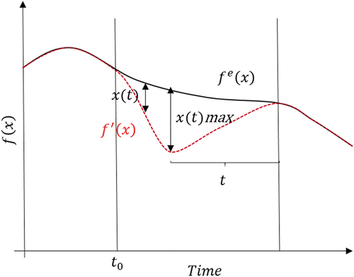
Let us assume that a disturbance affects the system at time t₀, displacing the system behaviour from x_t to x_tmax (see Figure 2). If the equilibrium is stable, then the system will eventually return to its original behaviour, and there is a maximum displacement x_max after which the system starts to bounce back (recover). The impact (I) is equal to x_max (see Figure 2) and can be calculated as the maximum Euclidean distance between the behaviour of the system in equilibrium $f^e\left(x\right)$ and the behaviour affected by the disturbance $f{ }^{\mathrm{\prime }}\left(x\right)$, as shown in Equation 1(1) $I=x_{max}=Max\left|f^e\left(x\right)-f{ }^{\mathrm{\prime }}\left(x\right)\right|$(1) .

(1) $I=x_{max}=Max\left|f^e\left(x\right)-f{ }^{\mathrm{\prime }}\left(x\right)\right|$(1)

Figure 2. Illustrative behaviour of a stable system after being affected by a disturbance with a limited duration.

The average recovery rate $R^{avg}$ is the average rate at which a system returns to equilibrium (Arnoldi et al., 2016; Herrera, 2017; Martin, Deffuant & Calabrese, 2011). Since the response is assumed to be asymptotic rather than linear, $R^{avg}$ can be estimated (see Equation 2)(2) $R^{avg}=\frac{ln{x}_t-ln{x}_0}{t}$(2) using the Euclidean norm $x\left(t\right)=\sqrt{\sum _i{x}_i^2\left(t\right)}$ to measure the phase-space distance to equilibrium. A more stable system returns faster to equilibrium, so the larger $R^{avg}$ is, the higher the system’s resilience.

(2) $R^{avg}=\frac{ln{x}_t-ln{x}_0}{t}$(2)

where:

$x_t$ is the distance to equilibrium N* for the function F(t)

t is the time it takes the system to bounce back.

To conceptualise the disturbance ($\sigma )$ affecting the system, we used a vector with two components (see Equation 3)(3) $\sigma =M\ast d$(3) : a) the magnitude of the disturbance (M) over b) a given period (d = duration) (Herrera, 2017). For example, if we assume σ is a drought, then M is the magnitude of the drought as a percent reduction below average rainfall expected for that period, and d is duration of the drought in months. In this paper, we are interested in the effect that a shock might have on the system rather than the effect of a long-term disturbance, and hence, we have assumed that $\sigma$ has a defined d.

(3) $\sigma =M\ast d$(3)

3.3. Scope definition: Resilience of what to what?

A first step in resilience assessment is to define the relationship of the resilience (Helfgott, 2018; Herrera de Leon & Kopainsky, 2019; Walker et al., 2004). Our analysis focuses on the resilience of two system outcomes: food production throughput and socioeconomic benefits of the system. To measure food production throughput, we decided to use the variable “calves exported”. It is worth noting that most of the cattle exported to the Italian market for veal are exported alive; therefore, we decided to measure the variable “calves exported” in livestock units rather than the weight of carcasses.

While the socioeconomic benefits of the system are more difficult to measure, we found it important to evaluate a variable that would allow us to evaluate the system from the perspective of the communities hosting the farms. With this purpose, we chose to use the variable “jobs in farms” as a proxy for measuring the socioeconomic benefits of farms to the region. Note that in the case of family farms, the number of jobs generated by a farm is estimated based on the total number of full-time equivalents working on the farm, including paid employees and family members. Using jobs allows us to narrow the benefits of farming systems to those directly perceived by the rural communities hosting them.

We looked at the combination of disturbances to the supply side resulting from climate change and long-term variations in consumption habits from the demand side. We used drought as the potential climate change effect that could reduce supply throughput. Similar many other European countries, France has been affected in recent years by more severe and frequent droughts that have adversely affected grasslands. The severity and frequency of extreme weather conditions are expected to continue to increase because of climate change, representing an increasing and unpredictable threat to farmers.

For analysis purposes, we considered the system’s response to a single disturbance that will temporarily reduce crop yield for a fixed period. Namely, we looked at the impact that one severe drought may have in the next 20 years. To do this, we tested system behaviour when exposed to different reductions in rainfall (M) from 0 mm/year to −200 mm/year and lasting from zero to three years (d), as shown in Table 1.

Table 1. Disturbances tested in the model where the disturbance $\sigma$ is defined as per Equation (1)(1) $I=x_{max}=Max\left|f^e\left(x\right)-f{ }^{\mathrm{\prime }}\left(x\right)\right|$(1) as the product of the magnitude of the disturbance (M) and its duration (d) and the angle (θ) between the vector components M and d.

Magnitudes durations	0mm/year	−10mm/year	−50mm/year	−100mm/year	−150mm/year	−200mm/year
1 year	0 mm/ θ: 0°	−10 mm/ θ: −5.7°	−50 mm/ θ: −26°	−100 mm/ θ: −45°	−150 mm/ θ: −56°	−200 mm/ θ: −63°
2 years	0 mm/ θ: 0°	−20 mm/ θ: −2.9°	−100 mm/ θ: −14°	−200 mm/ θ: −27°	−300 mm/ θ: −36°	−400 mm/ θ: −45°
3 years	0 mm/ θ: 0°	−30 mm/ θ: −1.9°	−150 mm/ θ: −9.4°	−300 mm/ θ: −18°	−450 mm/ θ: −26°	−600 mm/ θ: −34°

Note that since M has units of mm/year, the disturbances $\sigma$ have units of mm. The angle θ in Table 1 represents the angle between the vector components M and d. We cannot assume that the system will react in the same way to two vectors that have the same magnitude (e.g., $\sigma$ = −200 mm) if their angles are different (e.g., M = −100 mm/year with d = 2 years and M = −200 mm/year with d = 1 year).

Long-term changes to the consumption patterns were introduced in the model through scenarios affecting the operating environment in which bovine livestock systems operate. While we are mainly interested in changes to consumption habits, particularly the consumption of bovine meat, it became quickly apparent that changes in consumption will be part of a wider trend that involves changes in many different parts of the system. To account for these wider trends, we built on the narratives used by Mitter et al. (2020) to describe the shared socioeconomic pathways for European agriculture and food systems (Eur-Agri-SSPs). The Eur-Agri-SSPs are five scenarios outlining possible futures for key drivers affecting the responses of European food systems to climate change. The Eur-Agri-SSPs consider changes in several environmental, socioeconomic, and technical drivers based on the perspectives of different stakeholders (Mitter et al., 2020).

For simplicity, we only used the three Eur-Agri-SSPs that are more relevant to us by describing the most contrasting changes to bovine meat consumption patterns. The scenarios considered are:

1. Sustainable pathways: This scenario describes a significant increase in environmental awareness that translates into a considerable reduction in meat consumption per capita and a preference for locally produced food.

2. High-tech paths: This scenario portraits a future where growing faith on technological progress eases concerns about the effects of climate change and the consumption of meat per capita rebounds to increasing at rates seen in previous decades.

3. Established paths (business as usual): This is our counterfactual scenario. This scenario assumes consumption of meat per capita remains stable for the foreseeable future with an increase in total demand driven by a modest population growth.

These scenarios were introduced in the model by modifying the values of four variables: “land available for agriculture”, “market size”, “meat demand per capita”, and “farm’s technology”. Table 2 provides a short description of the narrative of each scenario and the variables that were used in the model to generate each of them.

Table 2. A summary of the Eur-Agri-SSPs scenarios used in the analysis to explore future trends for the bovine livestock system in the Bourbonnais region and the variables used in the model to generate each scenario.

SCENARIO	STORYLINE	VARIABLES AFFECTED IN THE MODEL
SCENARIO 1: AGRICULTURE ON SUSTAINABLE PATHS	Social and environmental awareness increase steadily and significantly and are reflected in tightened pro-environmental policies. European domestic demand shifts towards plant-based diets and bio-based materials. International trade decreases because short and transparent agricultural supply chains are preferred. Technology develops with a focus on reducing greenhouse gas emissions	Land available for agriculture: decreases 1% per year from 2020 Market size: decreases 1% per year from 2020 Meat demand per capita: decreases 2% per year from 2020 Farm’s technology: increases 1% per year from 2020
SCENARIO 2: AGRICULTURE ON ESTABLISHED PATHS	European development follows historical patterns resulting in slow but steady social, environmental, and technological progress. Agricultural commodities are mostly traded within Europe even though global market integration advances. Depletion of natural resources increases because of continuous growth of the agriculture and food economy, and pro-environmental regulations and resource-efficient technologies are only developed at a moderate pace.	Land available for agriculture: increases 0.5% per year from 2020 Market size: indexed to population growth in Europe. Meat demand per capita: remains at current levels. Farm’s technology: increases 0.5% per year from 2020
SCENARIO 3: AGRICULTURE ON HIGH-TECH PATHS	European residents share a growing faith in technology, material-intensive lifestyles, and trade liberalisation. Individuals’ affinity for technological innovation also affects increasing global demand for European agricultural products. Increased private investments in technological know-how and the education of employees in the agriculture and food systems boost economic growth, which is largely dependent on fossil energy sources.	Land available for agriculture: increases 0.1% per year from 2020 Market size: increases 3% per year from 2020 Meat demand per capita: remains at current levels. Farm’s technology: increases 2% per year from 2020

3.4. Definition of the system

The model developed for this case is an aggregated (as opposed to a detailed) interactive simulation model (Morecroft, 2007) and was built using historical data available in ‘Agreste (2020) describing the performance of beef production farms in the Bourbonnais. The structure of the model was built using cases described in the literature (e.g., Lien et al., 2007; Eakin & Wehbe, 2009) and stakeholder narratives collected although participatory workshops as part of the “Towards SUstainable and REsilient EU FARMing systems” (SURE-Farm) project, which is a research and innovation project funded by the European Union’s Horizon 2020 programme that involves 16 universities and research institutes from 11 European countries (SUREFarm, 2021).

At the core of the model, we have positioned the economic viability of farms represented by a reinforcing cycle between the number of “livestock units per farm” and “farm revenues” (see R1 in Figure 3). As pointed out by Bowman and Zilberman (2013), the factors determining whether a farm is profitable depend on the type of activity, technology used, and farmers’ management decisions. In our model, we started from the assumption that farmers will make choices that contribute to improving their profits by increasing their income and reducing their risk and labour requirements (Bowman & Zilberman, 2013; Stoorvogel et al., 2004).

Figure 3. A causal loop summarising reinforcing loops included in the model representing bovine livestock farms in Bourbonnais.

Note: Signs (“+” or ‘-‘) at arrowheads indicate the polarity of relationships: a “+” denotes that an increase in the independent variable causes the dependent variable to increase, ceteris paribus (and a decrease causes a decrease). Similarly, ‘-‘ denotes that an increase in the independent variable causes the dependent variable to decrease. The loop identifier, R, indicates a reinforcing feedback mechanism, and B indicates a balancing one (see Sterman, 2002).

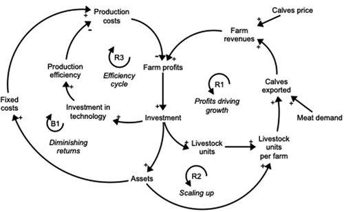
The rest of the model builds around this simple structure by searching which are the variables that are affecting and are affected by the variable “Farm profits”. We added these relationships by looking at case studies and theories documented in the literature that could explain past behaviour. Most of the dynamics included in the model are built upon the factors that farmers can influence directly to increase farm throughput. Farm throughput is a function of fixed inputs and different forms of farm capital, such as “Livestock units”, “Assets” (human capital and physical assets) and “Production efficiency”, driven by technological innovation (Ahituv & Kimhi, 2002). The model assumes that all things being equal, farmers that have a higher income will be more likely, more willing and able to increase their throughput by investing their profits into capital (Knowler & Bradshaw, 2007; Mccann et al., 1997),

For instance, it could be expected that larger farms (i.e., farms with more “Livestock units per farm”) have higher throughputs and higher revenues than smaller farms (see R1 in Figure 3). As discussed, by Bowman and Zilberman (2013), those farmers with higher revenues have more resources available for investing in either: a) continue increasing their size (R1), b) new technologies (e.g., automated feeders) that help them to increase efficiency and reduce operating costs (see R2 in Figure 3), or c) new assets (e.g., equipment, land, human capital) that enable them to increase the number of livestock units they can host in their farm (see R3 in Figure 3)

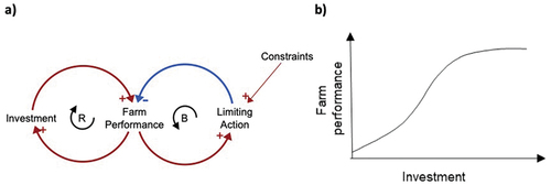
However, the relation between investment and efficiency gains is not linear. As the farms’ productivity approaches its limits, additional investment in new assets is likely to have a smaller impact on farms’ productivity. Eventually, the efficiencies gained through additional investment in new assets do not compensate for the return generated, and as shown in B1 (see Figure 3), lower returns slow down the investment in new assets.

This is a case of the limits to success mechanism described by Kim (2000, p. 7.) where “efforts initially lead to improved performance. Overtime, however, the system encounters a limit which causes the performance slow down or even decline” (see Figure 4). In this case, the limits are the maximum productivity per agricultural area that can be achieved through factors such as technology as even when a new technological breakthrough occurs, there is only so much food that can be produced from a given area.

Figure 4. a) A causal loop diagram illustrating the system archetype limits to success and b) an illustrative chart showing the expected relation between farm performance and investment.

There are other constraints limiting or slowing the system growth. For example, if all other variables remain constant, then an increase in the number and size of farms increases the “Workforce demand for farms” (see Figure 5). A higher demand for labour might increase competition in the labour market and increase recruitment costs and wages, slowing down further farm expansion (see B2 in Figure 5).

Figure 5. A causal loop summarising some balancing loops included in the model representing bovine livestock farms in Bourbonnais.

Arrows indicate the direction of causality. The plus (+) in the arrowhead indicates a direct relationship between variables, and the minus (-) indicates an inverse relationship between the variables connected. An “R” has been used to denote reinforcing loops and “B” to denote balancing loops.

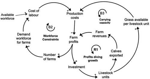
Similarly, there is only a maximum number of livestock units that the grasslands and water resources in the region can support (see B3 in Figure 5). Water quality and quantity have a direct effect on farming system production. Water availability is already a major concern for farmers (Falloon & Betts, 2010). More and larger farms are likely to consume more water, and farmers’ decisions about how to manage this resource may reduce water availability if, for example, farmers overexploit groundwater. Water quality may also worsen if fresh water sources are contaminated with nitrates due to more intensive practices (Howden et al., 2013). An increase in farm production may reduce water quality and water availability, reduce the grass available, and hinder future options for increasing production (see B3 in Figure 5). Correspondingly, farming systems need organic matter and nutrients present in the soil (Bot & Benites, 2005), but high production throughputs can result in soil degradation (Prager & Posthumus, 2010; Tsiafouli et al., 2015) and eventually increase farm dependency on fertilisers and production costs.

3.5. Constructing the simulation model

The timeline selected for the model was between 2000 and 2040, allowing us to calibrate the model against 20 years of historical data and to explore scenarios up to 20 years into the future. The delta time (DT), the parameter utilised by a numerical method (commonly Euler’s method) to numerically calculate the value of the stock, was set up as 1/12, equivalent to one month.

Model Inputs: Input variables are those that are not calculated by the model itself but are used as an input so that the model can calculate the remaining variables. In an SD model, there are often only a few parameters, as most variables are calculated within the model. Table 3 shows a summary of the main inputs to the model and the data used to calibrate the model by comparing simulated results against historical data.

Table 3. Summary of the main inputs and historical data used in the simulation model.

Variable	Use	Source	1999	2000	2001	2002	2003	2004	2005	2006	2007	2008	2009	2010	2011	2012	2013	2014	2015	2016
Utilised Agricultural Area (UAA) [Thousand ha]	Historic data	AGRESTE FDS_SAANR_1	-	503	-	-	-	495	494	490	488	490	488	486	484	484	483	-	-	-
UAA livestock and grassland [Thousand ha]	Historic data	AGRESTE FDS_SAANR_1	-	414	-	-	-	387	387	388	390	389	389	389	388	386	381	-	-	-
%UAA on lease [%]	Model Input	FADN SE030/SE025						77%	78%	78%	78%	77%	77%	77%	76%	77%	78%
Average price per ha (to buy) [Thousand €/ha]	Model Input	AGRESTE terre-net – AGRESTE	2	2	2	2	3	3	3	3	3	4	4	4	4	4	4	4	4	4
Average leasing [Thousand €/ha]	Model input	FADN SE375/SE025						86	92	89	90	91	92	91	92	96	96
Average wage farmer [Thousand €/FTE]	Model input	FADN SE370/SE010	-	-	-	-	-	3	2	2	2	2	2	2	2	2	2	-	-	-
Average farm’s operating cost [Thousand €//LU]	Model input	FADN SE281/SE080	-	-	-	-	-	0.41	0.40	0.39	0.41	0.44	0.47	0.45	0.48	0.55	0.55	-	-	-
Proportion of Assets vs. working capital [unitless]	Model input	FADN SE436/SE510						1.20	1.18	1.19	1.21	1.20	1.18	1.21	1.20	1.20	1.21
Average debt per farm [Thousand €]	Model input	FADN SE485	-	-	-	-	-	143	133	137	147	148	146	153	155	164	181	-	-	-
Average Livestock Units per farm [LU]	Historic data	AGRESTE FDS_SAANR_6, FDS_G_0001						88	92	96	101	106	109	114	114	118	122
Average number of calves per farm [LU]	Historic data	AGRESTE FDS_SAANR_6, FDS_G_0001						18	20	20	22	22	22	23	24	25	25
No. of inhabitants in the region [Thousand people]	Historic data	AGRESTE INSEE	345	345	345	344	344	344	343	343	343	343	342	342	343	341	341	341	340	339
Size of workforce [Thousand FTE]	Historic data	AGRESTE INSEE	-	-	-	-	-	-	-	-	-	-	-	-	199	-	-	-	-	208
No. of inhabitants working in farms (employees and self-employed) [Thousand FTE]	Historic data	AGRESTE FDS_RA_6005_4	-	10	10	10	10	10	10	10	10	10	10	10	-	-	-	-	-	-
Average rainfall precipitation (mm)	Model input	AGRESTE						820	518	723	691	821	640	921	662	817	955	813	580	808
Nb farms (cattle) [Thousand farms]	Historic data	AGRESTE FDS_G_0001	-	4	4	4	4	4	4	3	3	3	3	3	-	-	-	-	-	-

Historical data were used to validate outcomes produced by the model.

The stock and flow diagram in Figure 6 illustrates how the relationships described in the diagrams in Figures 3,5 were translated into an SD model using Stella architect software. The feedback loops in the figure are the same as those previously described as part of the definition of the system, but the stock diagram makes explicit which variables have been considered stocks (e.g., “Livestock units per farm”).

Figure 6. A simplified stock-and-flow diagram showing the main structure included in the simulation model representing livestock farming systems in Bourbonnais. Arrows indicate the direction of causality. The plus (+) in the arrowhead indicates a direct relationship between variables, and the minus (-) indicates an inverse relationship between the variables connected. An “R” has been used to denote reinforcing loops and “B” to denote balancing loops. Boxes represent stocks; arrows with valves represent flows. A stock is the accumulation of the difference between its inflows and outflows. Note that the actual model is more complex than this diagram.

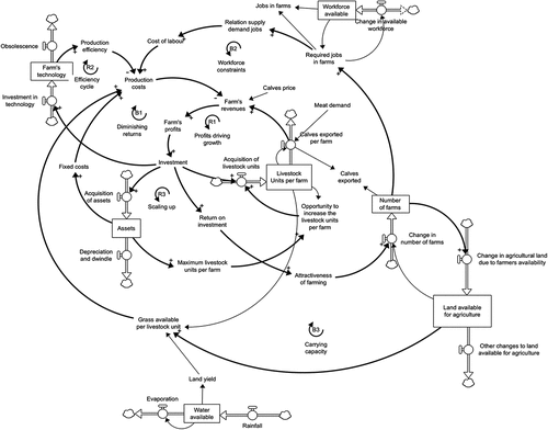
Figure 6 also shows exogenous factors included in the model. For example, the model considered changes in meat demand and water availability. These parts of the model are not internally driven by the mechanisms previously explained but by wider economic and environmental factors occurring at a larger scale than the one considered in the model (national and global as opposed to regional scale). For example, meat demand has changed according to the Eur-Agri-SSPs (see Figure 2). The opportunities for expanding the scope of the model and exploring long-term and larger-scale dynamics (e.g., the impact of sustainable farming technologies on climate change) are discussed later in this paper.

The diagram in Figure 6 is a map of the mathematical model developed in Stella software. Underneath this visual representation, the model has mathematical equations that recalculate the value for each variable every DT. The type of equation used will depend on the real-world nature of the relationships between variables (e.g., linear, exponential). Equations 4(4) $Clavesexported=Calvesexportedperfarm\times Numberoffarms$(4) ,5(5) $Farmprofits=Farmincome-ProductionCost$(5) show examples of the equations used in the model. Table A1 shows the full list of equations used in the model.

(4) $Clavesexported=Calvesexportedperfarm\times Numberoffarms$(4)

where:

Calves exported is the total amount of calves exported out of the Bourbonnais region, Calves exported per farm is the average amount of calves exported per farm, Number of farms is the number of bovine livestock farms operating at any given time.

(5) $Farmprofits=Farmincome-ProductionCost$(5)

where:

Farm profits: is the financial gain a farm makes from selling bovine livestock,

Farm income is the revenue a farm makes from selling bovine livestock, and

Production cost is the average annual cost incurred by the farm during the given time period.

The “stocks” represent variables that accumulate over time. In mathematical terms, a stock is the integral of the net flow added to the initial value of the stock, where the integral is calculated using numerical algorithms (see Equation 6). More details on numerical methods to calculate stocks in SD models can be found in Duggan (2016).

(6) $Assets\left(t\right)=Assets\left(t-dt\right)+\left(Acquisitionofassets-Depreciationanddwindle\right)\ast dt$(6)

where:

Assets (t) is a stock with the cumulative economic value of the assets owned by the farm, Acquisition of assets is a flow with the economic value of the assets added acquired by the farm, and Depreciation and dwindle is the loss of economic value due to ageing and obsolescence of the assets held by the farms.

Defining the initial value of the stock is an important step of the model calibration and can be done by using input variables (e.g., the known value of a stock at the beginning of the simulation) or, if there are no data available, by estimating the value of the stock that will represent an equilibrium between the initial inflow and outflow rates.

The model was validated using some of the tests recommended by Morecroft (2015), Sterman (2002), and Barlas (1996). Model validation is required to test to what extent the model can explain the system behaviour. As Barlas (1994) pointed out, in SD, the validation process focuses on the model structure and its capacity to capture patterns of behaviour rather than numerical predictions. The model structure was validated through the following structure-oriented tests: parameter-confirmation test, direct extreme-condition test, dimensional consistency test, extreme-condition test, and behaviour sensitivity test (Barlas, 1996).

The ability of the model to explain behaviour patterns was tested by comparing the model results against historical data. Figure 7 shows the simulated behaviour for selected variables in the model (dashed line) against the historical data obtained from the literature (solid line). As shown in the figure, both time series are close to each other and, more importantly, follow the same trend.

Figure 7. Simulated and historical behaviour for a) average farm size [ha/farm], b) number of farms [farms], c) Jobs in farms [FTE] and d) utilised agriculture area (UAA) [ha] (source for historical behaviour: Agreste FDS_G_0001).

To test behaviour precision, we used both error rate (E1) and error variance (E2). According to Qudrat-Ullah (2012), an SD model produces a good fit if E1 ≤5% and E2 ≤30%. The error rates for the selected variables are presented in Table 4. As seen in Table 4, both error rates are below the threshold, suggesting that the model offers a good fit.

Table 4. Model error for selected variables, where E1 is the error rate and E2 is the error variance.

Variable	E1	E2
UAA dedicated to livestock	0.6%	8.1%
Number farm jobs	0.7%	6.5%
Number livestock farms	1%	7.2%
Number of livestock units per farm	1.2%	10.8%

4. Results

4.1. Scenarios without additional climate change disturbance

Figure 8 shows simulation results for the two performance indicators: “jobs in farms” and “calves exported” in the absence of any disturbance. The solid lines in Figures 8a,b show the behaviour of these indicators under the established paths scenario (Scenario 2). As shown in the figures, without major changes in the socioeconomic landscape, the system continues its trajectory, and the system sees a small reduction in the number of people working on farms (Figure 8a) mainly due to the reduction in the proportion of family farms in the region. The decrease in the number of calves exported every year is more pronounced (see Figure 8b), as smaller farmers exit the industry due to poor returns resulting from more competitive markets.

Figure 8. Simulated behaviour for a) jobs on farms and b) calf exports under the three Eur-Agri-SSPs: Scenario 1 (Sc1): Agriculture on sustainable paths, Scenario 2 (Sc2): Agriculture on established paths, Scenario 3 (Sc3): Agriculture on high-tech paths.

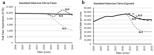
The simulated behaviour for the sustainable paths scenario (Scenario 1), dashed lines in Figures 8a,b, shows the effects a substantial reduction in the meat consumption per capita may have in the system. As expected, a decrease in demand results in a reduction in both variables (see Figure 8(a,b)) as the number of farms shrinks.

The high-tech paths scenario (Scenario 3) shows only moderate differences against the business as usual situation (Scenario 2). In the short-term, intensification and opportunities to export to new markets increase throughput (see Figure 8(b)) and reduce dependency on labour (see Figure 8(a)). However, as the number of farmers increases, the number of jobs bounces back, temporarily generating even more jobs that could be expected in the established paths scenario. However, in the medium term, the same openness to markets and globalisation are also likely to result in a more competitive environment. The diminishing returns mechanism and the lower production costs in other regions (e.g., Brazil, Argentina) are eventually too high for local producers, and both throughput and jobs start to decline back to the trend seen in the established paths scenario.

4.2. Scenarios with climate change disturbances

Figure 9 illustrates how the different droughts described in Table 1 could affect the behaviour of the system. For simplicity, Figure 9 only shows the simulation results under Scenario 2 (agriculture on established paths), since this is the scenario that closely resembles business-as-usual. The solid black line in Figure 9a,b is the expected behaviour without any disturbance (same as shown in Figure 8). The grey lines show the behaviour when the disturbance takes different combinations for magnitude and duration, and the red line shows the simulation run with the largest impact (I).

Figure 9. Simulated behaviour for a) jobs on farms and b) calf exports for the disturbances listed in Table 1 under Eur-Agri-SSPs 2 (Agriculture on established paths).

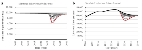
The time series resulting from simulations for different disturbance combinations under different scenarios were subsequently used to estimate the system resilience. System resilience was assessed using the metrics described in the methodology section, and the results can be found in Table 5. These results show that if the disturbance affecting the system is small, the impact on both variables is relatively low, and the recovery rate is high. In contrast, long durations result in high impact rates and slow recovery rates. The results also show that in some cases, the system has a higher resilience (lower I and higher R^avg) in Scenario 1.

Table 5. Resilience metrics for the disturbances tested in this analysis.

Magnitude [mm/year]	Duration [year]	Impact (I)						Average recovery rates
		Jobs lost [FTE]			Exports lost [LU/year]			Jobs created [FTE/year]			Exports recovered [LU/year^2]
		Scenario 1	Scenario 2	Scenario 3	Scenario 1	Scenario 2	Scenario 3	Scenario 1	Scenario 2	Scenario 3	Scenario 1	Scenario 2	Scenario 3
10	1	25	3	23	59	47	53	12	1	6	54	43	24
50	1	111	11	100	1,469	1,175	661	67	7	34	130	104	59
100	1	217	22	195	2,938	2,350	1,322	82	8	41	573	458	258
150	1	320	32	288	4,407	3,526	1,983	103	10	52	717	574	323
200	1	423	42	381	5,876	4,701	2,644	118	12	59	717	574	323
10	2	99	10	89	116	93	81	44	4	22	111	89	78
50	2	475	48	428	1,155	924	809	116	12	58	222	178	155
100	2	918	92	826	2,888	2,310	3,177	150	15	75	347	382	382
150	2	1,335	134	1,469	5,776	4,621	4,043	100	10	50	556	612	389
200	2	1,727	173	1,900	8,664	6,931	10,397	121	12	61	556	612	667
10	3	219	22	241	168	84	202	69	7	35	54	59	65
50	3	1,028	103	1,131	4,206	2,103	5,047	125	13	63	496	546	595
100	3	1,919	192	2,111	8,411	4,206	10,093	169	17	85	661	727	793
150	3	2,693	269	2,962	12,617	6,309	15,140	218	22	109	740	814	888
200	3	3,645	365	4,010	16,823	8,412	20,188	233	23	117	793	872	952

5. Analysis and discussion

As could be expected, bovine livestock systems, such as those in the Bourbonnais, are expected to perform better in scenarios with high meat consumption (Scenarios 2 and 3 in this paper) and to struggle in scenarios where plant-based diets are widespread (Scenario 1 in this paper). While scenarios with low meat production may be beneficial to some stakeholders, farmers and those depending on livestock farms for their living see them as an existential threat.

We argue, however, that this is not necessarily true once unpredictable effects of climate change are considered as the performance of the system in terms of outcomes differs from its performance in terms of resilience. As shown by the metric impact (I) in Table 5, after introducing unpredictable effects of climate change, the outcomes for both indicators (“jobs in farms” and “calves exported”) could be expected to be better under Scenario 1 (sustainable pathways). This resilience seems to be driven by the number of farms (see Figure 5). Since there is a smaller number of farms sharing the same environmental resources, especially water, a reduction in the availability of these resources has a smaller impact on the farms’ performance. It seems that, unintentionally, Scenario 1 has already moved the system to a more stable equilibrium where the system has a larger headroom regarding its environmental resources.

The results for the average recovery rate $R^{avg}$ in Table 5 are less conclusive. On the one hand, the model anticipates that the $R^{avg}$ for “jobs in farms” could be lower for Scenario 1 than for the other scenarios. This is not surprising because one of the assumptions in Scenario 1 is that barriers to entry for farmers are higher due to stricter environmental regulations. Hence, it could be expected that severe droughts will have smaller but more enduring consequences on jobs in Scenario 1 than in the other scenarios.

On the other hand, the $R^{avg}$ for “calves exported” is similar for all the scenarios, and the system seems to obtain a better combination of impact (I) and average recovery rate ($R^{avg}$) under Scenario 1 since the impacts are low, and the recovery is as quick as in the other scenarios. In Scenario 1, farmers are less likely to exit the system because there are strong entrance barriers to other competitors in the local markets and thus their products have high margins. This means that even if there is an external disturbance affecting their throughput, then the impact on farms’ profits and market position will be smaller and/or shorter.

The opposite happens in Scenario 3 (see Table 5), where impact (I) is high because the profit margin on the “calves exported” is low and markets are open and highly competitive. Under Scenario 3, we can expect that even a small reduction in the throughput may put farmers out of business. However, the same openness of markets assumed in Scenario 3 allows for a quick recovery (high $R^{avg}$) following the end of the disturbance. This quick recovery is the result of a larger market with a higher demand for meat and low entrance barriers.

In short, our results show that the scale and intensity of bovine livestock systems make them vulnerable to external disturbances such as climate change. Strategies focus only on improving their short-term performance, such as those expected in a high tech path (Scenario 3), may succeed in the short and medium term but are likely to increase some of these vulnerabilities, especially among smaller producers.

6. Conclusions and further research

The landscape of food production systems in Europe is rapidly changing as the social, environmental, and economic systems they are embedded in evolve. Bovine livestock systems are now constantly contested as environmental awareness reduces meat and milk consumption per capita and external disturbances such as climate change and the COVID-19 pandemic. The future subsistence of these farming systems that have traditionally defined the culture, economy, and landscape of many regions in Europe requires us to rethink their size and configuration. As our results suggest, these new systems require us to think beyond performance and to purposefully manage their resilience

As proposed in the introduction, the aim of our analysis was to determine the conditions under which bovine livestock systems, such as those in the Bourbonnais region, can persist sustainably. Our results suggest that, counterintuitively, this type of farming system has better chances to survive in the sustainable paths scenario (Scenario 1). On the one hand, the anticipated change in diets assumed in this scenario is likely to reduce the number of farms and jobs in the sector. However, the same downsizing of the system seems to increase its resilience to environmental threats, such as the effects of climate change, when compared to other scenarios. The results suggest that a reduction in the number of farmers operating in the region could give the system enough headroom to operate in more challenging conditions.

Unfortunately, livestock systems in Europe are likely to look different in the future, and although it may be counterintuitive to farmers and other stakeholders, managing the system transition towards a new stability domain may be a better alternative than cling to unsustainable and vulnerable paths. However, further work needs to be done to understand these new stability domains and to engage farmers in conversations that help them look beyond short-term subsistence.

Moreover, recognising the challenges ahead, it is also important that local and central governments facilitate the transformation of farming systems to this new stability domain by helping farmers and local communities endure the social and economic consequences of this change. Farmers and communities depending on farming systems are about to undergo significant and painful transformations, and more work needs to be done to understand the support that they will need. Further research will need to include wider stakeholder engagement, potentially using microworlds as transitional objects, to have open conversations between stakeholders with conflicting views.

Disclosure statement

No potential conflict of interest was reported by the author(s).

Supplementary material

Supplemental data for this article can be accessed online at https://doi.org/10.1080/17477778.2022.2083990

Additional information

Funding

This work was supported by the EU Horizon 2020 Food [727520].

Appendix

Table A1. Model equations.

TYPE	VARIABLE	EQUATION	STOCK INITIAL VALUE	UNITS	COMMENT
STOCK	Calves_in_utero[Farm_configuration](t)	Calves_in_utero[Farm_configuration](t – dt) + (Breeding[Farm_ configuration] – Calving_for_Milk[Farm_configuration] – Calving_for_meat_production[Farm_configuration]) * dt	INIT Calves_in_utero[Farm_configuration] = “Initial_Livestock_(LU)”*Livestock_aging_chain_distribution[Calvesinutero]	livestockunit
STOCK	Cows_for_Meat[Farm_configuration](t)	Cows_for_Meat[Farm_configuration](t – dt) + (Calving_for_meat_production[Farm_configuration] + Bought_fattening_cattle[Farm_configuration] – slaughtering_rate[Farm_configuration]) * dt	INIT Cows_for_Meat[Farm_configuration] = (Livestock_aging_chain_distribution[Calves]*”Initial_Livestock_(LU)”+Livestock_aging_chain_distribution[Heifers]*”Initial_Livestock_(LU)”+Livestock_aging_chain_distribution[Mature]*”Initial_Livestock_(LU)”)*(1-Fraction_of_Calves_for_Milk_Production)	livestockunit
STOCK	Mature_Milk_Cows[Farm_configuration](t)	Mature_Milk_Cows[Farm_configuration](t – dt) + (First_Calving[Farm_configuration] – Culling_Milk_Cows[Farm_configuration]) * dt	INIT Mature_Milk_Cows[Farm_configuration] = “Initial_Livestock_(LU)”*Livestock_aging_chain_distribution[Mature]*Fraction_of_Calves_for_Milk_Production	livestockunit
STOCK	Milk_Calves[Farm_configuration](t)	Milk_Calves[Farm_configuration](t – dt) + (Calving_for_Milk[Farm_configuration] – Maturing[Farm_configuration]) * dt	INIT Milk_Calves[Farm_configuration] = “Initial_Livestock_(LU)”*Livestock_aging_chain_distribution[Calves]*Fraction_of_Calves_for_Milk_Production	livestockunit
STOCK	Milk_Heifers[Farm_configuration](t)	Milk_Heifers[Farm_configuration](t – dt) + (Maturing[Farm_configuration] + Bought_Heifers[Farm_configuration] – First_Calving[Farm_configuration]) * dt	INIT Milk_Heifers[Farm_configuration] = “Initial_Livestock_(LU)”*Livestock_aging_chain_distribution[Heifers]*Fraction_of_Calves_for_Milk_Production	livestockunit
FLOW	Bought_fattening_cattle[Farm_configuration]	Change_in_cows_for_meat+slaughtering_rate-Calving_for_meat_production		livestockunit/Years
FLOW	Bought_Heifers[Farm_configuration]	MAX(Heifers_to_increase_milk_LU+Culling_Milk_Cows-Calving_for_Milk, 0)		livestockunit/Years
FLOW	Breeding[Farm_configuration]	Mature_Milk_Cows/Years_between_breeding		livestockunit/Years
FLOW	Calving_for_meat_production[Farm_configuration]	Calves_in_utero/Pregnancy_Time*(1-Fraction_of_Calves_for_Milk_Production)		livestockunit/Years
FLOW	Calving_for_Milk[Farm_configuration]	Calves_in_utero/Pregnancy_Time*Fraction_of_Calves_for_Milk_Production		livestockunit/Years
FLOW	Culling_Milk_Cows[Farm_configuration]	Mature_Milk_Cows/Fattering_time_Milk_Cow		livestockunit/Years
FLOW	First_Calving[Farm_configuration]	Milk_Heifers/Time_between_Calves		livestockunit/Years
FLOW	Maturing[Farm_configuration]	Milk_Calves/Maturing_Time		livestockunit/Years
FLOW	slaughtering_rate[Farm_configuration]	Cows_for_Meat/Fattering_Time		livestockunit/Years
DATA	Average_Fattening_time[Farm_configuration]	2		Years
EQUATION	Average_Weigh_per_cow[Farm_configuration]	Initial_Average_weight_per_LU*Effect_of_fattening_time_on_weight* Effect_of_forage_availability_on_weight		Ton/livestockunit
EQUATION	Average_weight_milk_cow[Farm_configuration]	Initial_Average_weight_per_LU*Effect_of_fattening_time_on_weight_milk_cow* Effect_of_forage_availability_on_weight_milk_cows		Ton/livestockunit
EQUATION	Biomass_Grasslands_available_Livestock[Farm_configuration]	Land.Grassland_Area*Grassland_yield		Ton/years
EQUATION	Change_in_cows_for_meat[Farm_configuration]	(Finance.Desired_LU_meat-Cows_for_Meat)/Time_to_Adjust_Livestock		livestockunit
EQUATION	Desired_Livestock[Farm_configuration]	Land.Area_Livestock*.022		livestockunit
EQUATION	Claves exported	Calves exported per farm × Number of farms		livestockunit/Years
EQUATION	Calves exported per farm	Cows for meat/dt		livestockunit/Years/Farm
TIME SERIES	Effect_of_fattening_time_on_weight[Farm_configuration]	GRAPH(Relative_Fattening_time) Points: (0.000, 0.000), (0.200, 0.242), (0.400, 0.500), (0.600, 0.700), (0.800, 0.900), (1.000, 1.000), (1.200, 1.050), (1.400, 1.100), (1.600, 1.125), (1.800, 1.150), (2.000, 1.150)		Dimensionless
EQUATION	Farm profits	Farm income -Production Cost		Euros/Years
TIME SERIES	Effect_of_fattening_time_on_weight_milk_cow[Farm_configuration]	GRAPH(Relative_Fattening_time_Milk_Cows) Points: (0.000, 0.000), (0.200, 0.242), (0.400, 0.500), (0.600, 0.700), (0.800, 0.900), (1.000, 1.000), (1.200, 1.050), (1.400, 1.100), (1.600, 1.125), (1.800, 1.150), (2.000, 1.150)		Dimensionless
TIME SERIES	Effect_of_forage_availability_on_Milk_production_cost[Farm_configuration]	GRAPH(Percentage_of_forage_requirement_fulfilled) Points: (0.8000, 0.431), (0.8200, 0.600), (0.8400, 0.708), (0.8600, 0.800), (0.8800, 0.869), (0.9000, 0.920), (0.9200, 0.980), (0.9400, 1.000), (0.9600, 1.000), (0.9800, 1.000), (1.0000, 1.000)		Dimensionless
TIME SERIES	Effect_of_forage_availability_on_weight[Farm_configuration]	GRAPH(SMTH3(Percentage_of_forage_requirement_fulfilled, Average_Fattening_time)) Points: (0.8000, 0.431), (0.8200, 0.600), (0.8400, 0.680), (0.8600, 0.750), (0.8800, 0.820), (0.9000, 0.869), (0.9200, 0.900), (0.9400, 0.940), (0.9600, 0.980), (0.9800, 1.000), (1.0000, 1.000)		Dimensionless
STOCK	Assets(t)	Assets (t – dt) + (Acquisition of assets – Depreciation and dwindle) * dt	INIT Assets = Initial_Capital_Stock	Euros
TIME SERIES	Effect_of_forage_availability_on_weight_milk_cows[Farm_configuration]	GRAPH(SMTH3(Percentage_of_forage_requirement_fulfilled, Fattering_time_Milk_Cow)) Points: (0.8000, 0.431), (0.8200, 0.600), (0.8400, 0.680), (0.8600, 0.750), (0.8800, 0.820), (0.9000, 0.869), (0.9200, 0.900), (0.9400, 0.940), (0.9600, 0.980), (0.9800, 1.000), (1.0000, 1.000)		Dimensionless
DATA	“Farm_Size_(LU/UAA)”[Farm_configuration]	0.0216		livestockunit/km2	An average of 52 LU in 88 ha (including 32 ha grassland)
DATA					http://www.filiere-laitiere.fr/en/key-figures/50-facts-about-french-dairy-industry
DATA	Fattering_Time	2		Years
DATA	Fattering_time_Milk_Cow	4		Years	Assumption
DATA					This assumption will need to be validated. The model behaviour is not sensitive to this assumption.
DATA	forage_intake_per_year	14		Ton/ (livestockunit*year)
DATA	Fraction_of_Calves_for_Milk_Production[Farm_configuration]	0.43		Dimensionless	Excel workbook
EQUATION	GAP_in_Livestock[Farm_configuration]	Finance.Desired_LU_Milk-Total_Milk_livestock_held		livestockunit
EQUATION	Grassland_yield[Farm_configuration]	Initial_Grassland_Yield_dry_matter*Soil.Effect_of_Water_on_Yield		Ton/(Km2*year)
EQUATION	Heifers_to_increase_milk_LU[Farm_configuration]	GAP_in_Livestock/Time_to_Adjust_Livestock		livestockunit/Years
TIME SERIES	Historical_Beef_production	GRAPH(TIME) Points: (2005.00, 0.0), (2006.00, 0.0), (2007.00, 0.0), (2008.00, 0.0), (2009.00, 1490.16), (2010.00, 1519.25), (2011.00, 1557.07), (2012.00, 1477.69), (2013.00, 1404.49), (2014.00, 1419.16), (2015.00, 1452.77), (2016.00, 1464.15), (2017.00, 1442.18), (2018.00, 0.0), (2019.00, 0.0), (2020.00, 0.0)		Thousand Ton/Years
DATA	Initial_Average_weight_per_LU	0.75		Ton/livestockunit
DATA	Initial_Grassland_Yield_dry_matter	32		ton/(year*Km2)
EQUATION	“Initial_Livestock_(LU)”[Farm_configuration]	“Farm_Size_(LU/UAA)”*INIT(Land.Area_Livestock)		livestockunit
DATA	Livestock_aging_chain_distribution[Calves]	0.15		Dimensionless
DATA	Livestock_aging_chain_distribution[Heifers]	0.12		Dimensionless
DATA	Livestock_aging_chain_distribution[Mature]	0.73		Dimensionless
DATA	Livestock_aging_chain_distribution[Calvesinutero]	0.075		Dimensionless
DATA	Maturing_Time	1.5		Years
EQUATION	Milk_Demand_for_Calves[Farm_configuration]	Milk_Calves*Milk_demand_per_calve		Ton/years
DATA	Milk_demand_per_calve	0.45		Ton/ (years*livestockunit)
EQUATION	Milk_for_sale[Farm_configuration]	Milk_Production-Milk_Demand_for_Calves		Ton/years
EQUATION	Milk_Production[Farm_configuration]	Mature_Milk_Cows*Milk_Production_per_cow_per_year		Ton/years
DATA	Milk_Production_per_cow_per_year[Farm_configuration]	1.9		Ton/ (years*livestockunit)	A typical cow produces 6800 liters of milk a year
DATA
DATA					http://www.filiere-laitiere.fr/en/key-figures/50-facts-about-french-dairy-industry
EQUATION	Percentage_of_forage_requirement_fulfilled[Farm_configuration]	MIN(Biomass_Grasslands_available_Livestock/Required_Forage, 1)		Dimensionless
DATA	Pregnancy_Time	1		Years
TIME SERIES	Reference_mode_Total_Livestock	GRAPH(TIME) Points: (2005.00, 6,075,040), (2006.00, 6,200,000), (2007.00, 6,295,100), (2008.00, 6,300,000), (2009.00, 6,000,000), (2010.00, 5,557,420), (2011.00, 5,300,000), (2012.00, 5,000,000), (2013.00, 5,035,170), (2014.00, 5,100,000), (2015.00, 5,200,000), (2016.00, 5,460,730), (2017.00, 5,500,000)		livestockunit
TIME SERIES	Reference_model_Milk_for_sale	GRAPH(TIME) Points: (2005.00, 3,496,000), (2006.00, 3,496,000), (2007.00, 3,496,000), (2008.00, 3,496,000), (2009.00, 3,496,000), (2010.00, 3,472,000), (2011.00, 3,383,000), (2012.00, 3,564,000), (2013.00, 3,572,000), (2014.00, 3,391,000), (2015.00, 3,299,000), (2016.00, 3,294,000), (2017.00, 3,230,000)		Ton/years
EQUATION	Relative_Fattening_time[Farm_configuration]	Fattering_Time/Average_Fattening_time		Dimensionless
EQUATION	Relative_Fattening_time_Milk_Cows[Farm_configuration]	Fattering_time_Milk_Cow/Average_Fattening_time		Dimensionless
EQUATION	Required_Forage[Farm_configuration]	Total_Livestock*forage_intake_per_year		Ton/years
EQUATION	Sum_Livestock	SUM(Total_Livestock)		livestockunit
DATA	Time_between_Calves	0.75		Years
DATA	Time_to_Adjust_Livestock	5		Years	Assumption
DATA					This assumption will need to be validated. The model behaviour is not sensitive to this assumption.
EQUATION	Total_Livestock[Farm_configuration]	Total_Milk_livestock_held+Cows_for_Meat+Calves_in_utero		livestockunit
EQUATION	Total_meat_produced[Farm_configuration]	Total_meat_produced_Feeder_Cattle+Total_meat_produced_Milk_Cattle		Ton/years
EQUATION	Total_meat_produced_Feeder_Cattle[Farm_configuration]	slaughtering_rate*Average_Weigh_per_cow		Ton/years
EQUATION	Total_meat_produced_Milk_Cattle[Farm_configuration]	Culling_Milk_Cows*Average_weight_milk_cow		Ton/years
EQUATION	Total_Meat_throughput	SUM(Total_meat_produced)/1000		Ton/years
EQUATION	Total_Milk_for_Sale	SUM(Milk_for_sale)		Ton/years
EQUATION	Total_Milk_livestock_held[Farm_configuration]	Milk_Calves+Milk_Heifers+Mature_Milk_Cows		livestockunit
DATA	Years_between_breeding[Farm_configuration]	4		year
STOCK	“%_UAA_used_for_crops”[Farm_configuration](t)	“%_UAA_used_for_crops”[Farm_configuration](t – dt) + (- Change_in_use_of_land[Farm_configuration]) * dt	INIT “%_UAA_used_for_crops”[Farm_configuration] = 1-Initial_%_of_UAA_used_for_Livestock	Dimensionless
STOCK	“%_UAA_used_for_livestock”[Farm_configuration](t)	“%_UAA_used_for_livestock”[Farm_configuration](t – dt) + (Change_in_use_of_land[Farm_configuration]) * dt	INIT “%_UAA_used_for_livestock”[Farm_configuration] = Initial_%_of_UAA_used_for_Livestock	Dimensionless
STOCK	Desired_Km2_UAA[Farm_configuration](t)	Desired_Km2_UAA[Farm_configuration](t – dt) + (Change_on_Desired_UAA[Farm_configuration]) * dt	INIT Desired_Km2_UAA[Farm_configuration] = INIT(Finance.Desire_to_convert_arable_land)	km2
STOCK	No_Utilised_Agricultural_Area(t)	No_Utilised_Agricultural_Area(t – dt) + (- Change_of_agricultural_area[1] – Change_of_agricultural_area[2] – Change_of_agricultural_area[3] – Change_of_agricultural_area[4] – Change_of_agricultural_area[5]) * dt	INIT No_Utilised_Agricultural_Area  = .06*SUM(Initial_Utilised_Agricultural_Area)	km2
STOCK	“Utilised_Agricultural_Area_(UAA)”[Farm_configuration](t)	“Utilised_Agricultural_Area_(UAA)”[Farm_configuration](t – dt) + (Change_of_agricultural_area[Farm_configuration]) * dt	INIT “Utilised_Agricultural_Area_(UAA)”[Farm_configuration] = Initial_Utilised_Agricultural_Area	km2
EQUATION	Change_in_use_of_land[Farm_configuration]	GAP_%_UAA_for_Livestock/Time_to_adjust_farming_activity		person/(person*year)
EQUATION	Change_of_agricultural_area[Farm_configuration]	MIN(No_Utilised_Agricultural_Area/DT, Arable_Land_Gap)		km2/years
EQUATION	Change_on_Desired_UAA[Farm_configuration]	(Finance.Desire_to_convert_arable_land-Desired_Km2_UAA)/Time_to_adjust_Perception		km2/years
EQUATION	Arable_Land_Gap[Farm_configuration]	(Desired_Km2_UAA-”Utilised_Agricultural_Area_(UAA)”)/Time_to_Adjust_Demand		km2/years
EQUATION	Area_for_Crops_and_Grain[Farm_configuration]	MAX(“%_UAA_used_for_crops”*”Utilised_Agricultural_Area_(UAA)”, 0)		km2
EQUATION	“Area_for_livestock_(including_Grasslands)”[Farm_configuration]	“Utilised_Agricultural_Area_(UAA)”*MIN(“%_UAA_used_for_livestock”, 1)		km2
EQUATION	Area_Livestock[Farm_configuration]	Relation_area_livestock_vs_area_Grassland*”Area_for_livestock_(including_Grasslands)”		km2
EQUATION	GAP_%_UAA_for_Livestock[Farm_configuration]	Finance.Desired_Area_for_Livestock_and_grassland*Finance.Effect_of_crops_gross_margin_on_development_of_Livestock/”Utilised_Agricultural_Area_(UAA)”-”%_UAA_used_for_livestock”		Dimensionless
EQUATION	Grassland_Area[Farm_configuration]	“Area_for_livestock_(including_Grasslands)”*Relation_area_livestock_vs_area_Grassland		km2
DATA	Initial_%_of_UAA_used_for_Livestock[Farm_configuration]	0.63		Dimensionless
DATA	Initial_Utilised_Agricultural_Area[Farm_configuration]	171,510,400		km2
TIME SERIES	Reference_mode_Area_Livestock	GRAPH(TIME) Points: (2005.00, 562,962,000), (2006.00, 550,000,000), (2007.00, 576,405,000), (2008.00, 560,000,000), (2009.00, 550,000,000), (2010.00, 500,319,000), (2011.00, 500,000,000), (2012.00, 490,000,000), (2013.00, 465,470,000), (2014.00, 450,000,000), (2015.00, 480,000,000), (2016.00, 505,428,000), (2017.00, 530,000,000)		km2
TIME SERIES	Reference_mode_Total_UAA	GRAPH(TIME) Points: (2005.00, 860,514,000), (2006.00, 8.6e+08), (2007.00, 876,684,000), (2008.00, 8.5e+08), (2009.00, 8.4e+08), (2010.00, 822,479,000), (2011.00, 8e+08), (2012.00, 7.7e+08), (2013.00, 764,036,000), (2014.00, 7.8e+08), (2015.00, 8.1e+08), (2016.00, 821,257,000), (2017.00, 8.1e+08)		km2
DATA	Relation_area_livestock_vs_area_Grassland[1]	0.5		Dimensionless
DATA	Relation_area_livestock_vs_area_Grassland[2]	0.5		Dimensionless
DATA	Relation_area_livestock_vs_area_Grassland[3]	0.5		Dimensionless
DATA	Relation_area_livestock_vs_area_Grassland[4]	0.5		Dimensionless
DATA	Relation_area_livestock_vs_area_Grassland[5]	0.5		Dimensionless
DATA	Time_to_Adjust_Demand	3		year
DATA	Time_to_adjust_farming_activity	10		year
DATA	Time_to_adjust_Perception	1		Years
EQUATION	Total_Area_Livestock	SUM(“Area_for_livestock_(including_Grasslands)”)		km2
EQUATION	Total_UAA	SUM(“Utilised_Agricultural_Area_(UAA)”)		km2
STOCK	Soil_Organic_Carbon[Farm_configuration](t)	Soil_Organic_Carbon[Farm_configuration](t – dt) + (Soil_Organic_Carbon_Input[Farm_configuration] – Organic_Carbon_Mineralisation_rate[Farm_configuration]) * dt	INIT Soil_Organic_Carbon[Farm_configuration] = 12.5	Ton/(Km2)
STOCK	Soil_Organic_Nitrogen[Farm_configuration](t)	Soil_Organic_Nitrogen[Farm_configuration](t – dt) + (Soil_Organic_Nitrogen_Input[Farm_configuration] – Soil_Organic_Nitrogen_Mineralisation_Rate[Farm_configuration]) * dt	INIT Soil_Organic_Nitrogen[Farm_configuration] = 2.6	Ton/(Km2)
FLOW	Organic_Carbon_Mineralisation_rate[Farm_configuration]	Soil_Organic_Carbon/Average_Carbon_Mineralisation_Time		Ton/(Km2*year)
FLOW	Soil_Organic_Carbon_Input[Farm_configuration]	Organic_Matter_from_Livestock_Manure*Carbon_Share_in_Dry_Matter		Ton/(Km2*year)
FLOW	Soil_Organic_Nitrogen_Input[Farm_configuration]	Organic_Nitrogen_from_livestock_manure		Ton/(Km2*year)
FLOW	Soil_Organic_Nitrogen_Mineralisation_Rate[Farm_configuration]	Soil_Organic_Nitrogen/Nitrogen_Mineralisation_Time		Ton/(Km2*year)
DATA	Add_climate_change_effect	0		Dimensionless
DATA	Average_Carbon_Mineralisation_Time	35		Years
DATA	Carbon_Share_in_Dry_Matter	0.1		Dimensionless
DATA	Effect_of_climate_change	1		Dimensionless
EQUATION	Effect_of_Nitrogen_on_yield[Farm_configuration]	MIN((Nitrogen_Plant_Uptake/Standard_N_required)^Yield_sensitivity_to_Nitrogen, Max_effect_of_Nitrogen_on_Yield)		Dimensionless
DATA	Effect_of_OM_in_Nitrogen_Uptake	0.25		Dimensionless
DATA	Effect_of_OM_in_Water_uptake	0.25		Dimensionless
EQUATION	Effect_of_Water_on_Yield[Farm_configuration]	MIN((Water_Plant_Uptake*Land.Area_for_Crops_and_Grain/Standard_Water_Required)^Yield_sensitivity_to_Water, Max_effect_of_Water_on_Yield)		Dimensionless
DATA	Initial_Plant_Nitrogen_uptake	0.5		Dimensionless
DATA	Initial_Plant_Water_Uptake	0.5		Dimensionless
EQUATION	Initial_Soil_Organic_Matter[Farm_configuration]	INIT(Soil_Organic_Matter)		Ton/(Km2)
DATA	Max_effect_of_Nitrogen_on_Yield	1		Dimensionless
DATA	Max_effect_of_Water_on_Yield	1		Dimensionless
DATA	Nitrogen_content_of_livestock_manure	0.2		Dimensionless
EQUATION	Nitrogen_Mineral[Farm_configuration]	Soil_Organic_Nitrogen_Mineralisation_Rate+Tons_Chemical_Fertilisers_used		Ton/(Km2*year)
DATA	Nitrogen_Mineralisation_Time	35		year
EQUATION	Nitrogen_Plant_Uptake[Farm_configuration]	Nitrogen_Mineral*Plant_uptake_share_of_Nitrogen_Min		Ton/(Km2*year)
EQUATION	Organic_Matter_from_Livestock_Manure[Farm_configuration]	Livestock.Total_Livestock*Tons_Manure_per_LU/(Land.Area_for_Crops_and_Grain+Land.Grassland_Area)		Ton/(Km2*year)
EQUATION	Organic_Nitrogen_from_livestock_manure[Farm_configuration]	Nitrogen_content_of_livestock_manure*Organic_Matter_from_Livestock_Manure		Ton/(Km2*year)
EQUATION	Oscilations	SINWAVE(MAX(Effect_of_climate_change-1, 1), 10/Effect_of_climate_change)		Dimensionless
EQUATION	Percentage_of_Area_held_each_FS[Farm_configuration]	Land.Initial_Utilised_Agricultural_Area/SUM(Land.Initial_Utilised_Agricultural_Area)		Dimensionless
EQUATION	Plant_uptake_share_of_Nitrogen_Min[Farm_configuration]	Initial_Plant_Nitrogen_uptake*Relative_Organic_Matter^Effect_of_OM_in_Nitrogen_Uptake		Dimensionless
EQUATION	Plant_uptake_share_water[Farm_configuration]	Initial_Plant_Water_Uptake*Relative_Organic_Matter^Effect_of_OM_in_Water_uptake		Dimensionless
EQUATION	Rainfall_Precipitation	619*(1+ STEP(Oscilations, 2018)*Add_climate_change_effect)-STEP(250, 2008)+STEP(500, 2010)-STEP(250, 2018)		mm/year
EQUATION	Relative_Organic_Matter[Farm_configuration]	Soil_Organic_Matter/Initial_Soil_Organic_Matter		Dimensionless
EQUATION	Soil_Organic_Matter[Farm_configuration]	Soil_Organic_Carbon*Carbon_Share_in_Dry_Matter		Ton/(Km2)
DATA	Standard_N_required	6		Ton/(Km2*year)
EQUATION	Standard_Water_Required[Farm_configuration]	Water_Required_per_Km2_grassland*Land.Grassland_Area+Water_Required_per_Km2_crop_arable_land*Land.Area_for_Crops_and_Grain		Ton/(Km2*year)
DATA	Tons_Chemical_Fertilisers_used[1]	0.25		Ton/(Km2*year)
DATA	Tons_Chemical_Fertilisers_used[2]	0.25		Ton/(Km2*year)
DATA	Tons_Chemical_Fertilisers_used[3]	0.25		Ton/(Km2*year)
DATA	Tons_Chemical_Fertilisers_used[4]	0.25		Ton/(Km2*year)
DATA	Tons_Chemical_Fertilisers_used[5]	0.25		Ton/(Km2*year)
DATA	Tons_Manure_per_LU	0.025		ton/(livestockunit*year)
EQUATION	Total_Cost_Fertilisers[Farm_configuration]	Market.Fertilisers_Price*Total_Demand_Fertilisers		Euros/Years
EQUATION	Total_Demand_Fertilisers[Farm_configuration]	Tons_Chemical_Fertilisers_used*(Land.Area_for_Crops_and_Grain+Land.Grassland_Area)		Ton/years
EQUATION	Water_Plant_Uptake[Farm_configuration]	MAX(Rainfall_Precipitation*Plant_uptake_share_water, 0)		mm/year
DATA	Water_Required_per_Km2_crop_arable_land	325		mm
DATA	Water_Required_per_Km2_grassland	250		mm
DATA	Yield_sensitivity_to_Nitrogen	0		Dimensionless
DATA	Yield_sensitivity_to_Water	0.25		Dimensionless
STOCK	Account_payable[Farm_configuration](t)	Account_payable[Farm_configuration](t – dt) + (No_Cash_Expenses[Farm_configuration] – Payments_to_suppliers[Farm_configuration]) * dt	INIT Account_payable[Farm_configuration] = 0.9*10^9	Euros
STOCK	Account_Receivable[Farm_configuration](t)	Account_Receivable[Farm_configuration](t – dt) + (Net_Sales[Farm_configuration] – Cash_receipts[Farm_configuration]) * dt	INIT Account_Receivable[Farm_configuration]  = INIT(Total_Revenues_Farming)*2/12	Euros
STOCK	Assets[Farm_configuration](t)	Assets[Farm_configuration](t – dt) + (PP&E_Purchase[Farm_configuration] – Depreciation[Farm_configuration]) * dt	INIT Assets[Farm_configuration] = 2*Initial_Capital_Stock	Euros
STOCK	Capital_Stock[Farm_configuration](t)	Capital_Stock[Farm_configuration](t – dt) + (Increase_Stakeholders_Equity[Farm_configuration]) * dt	INIT Capital_Stock[Farm_configuration] = Initial_Capital_Stock	Euros
STOCK	Cash[Farm_configuration](t)	Cash[Farm_configuration](t – dt) + (Cash_receipts[Farm_configuration] + Debt_acquired[Farm_configuration] + Equity_investment[Farm_configuration] – Cash_disbursements[Farm_configuration] – PP&E_Purchase[Farm_configuration] – Debt_Paid[Farm_configuration] – Dividends_paid[Farm_configuration]) * dt	INIT Cash[Farm_configuration] = 1.8*10^9	Euros
STOCK	Farmers_Debt[Farm_configuration](t)	Farmers_Debt[Farm_configuration](t – dt) + (Debt_increase[Farm_configuration] – Debt_reduction[Farm_configuration]) * dt	INIT Farmers_Debt[Farm_configuration]  = INIT(Cash)-Initial_Capital_Stock	Euros
STOCK	Retained_earnings[Farm_configuration](t)	Retained_earnings[Farm_configuration](t – dt) + (Total_Revenues[Farm_configuration] – Production_cost[Farm_configuration] – Income_tax_payable[Farm_configuration] – Dividends[Farm_configuration] – Operating_Expenses[Farm_configuration] – Interest_paid[Farm_configuration]) * dt	INIT Retained_earnings[Farm_configuration] = 800,000,000	Euros
FLOW	Cash_disbursements[Farm_configuration]	Payments_to_suppliers+Operating_Expenses+Income_tax_payable+Interest_paid		Euros/Years
FLOW	Cash_receipts[Farm_configuration]	Account_Receivable/(Average_credit_given*Convertion_days_to_years)		Euros/Years
FLOW	Debt_acquired[Farm_configuration]	Cash_required*Fraction_of_cash_cover_with_debt		Euros/Years
FLOW	Debt_increase[Farm_configuration]	Debt_acquired		Euros/Years
FLOW	Debt_Paid[Farm_configuration]	Debt_reduction		Euros/Years
FLOW	Debt_reduction[Farm_configuration]	Farmers_Debt/Average_debt_time		Euros/Years
FLOW	Depreciation[Farm_configuration]	Assets/Depreciation_time		Euros/Years
FLOW	Dividends[Farm_configuration]	Annual_return_paid*Retained_earnings/DT		Euros/Years
FLOW	Dividends_paid[Farm_configuration]	Dividends		Euros/Years
FLOW	Equity_investment[Farm_configuration]	Cash_required*(1-Fraction_of_cash_cover_with_debt)		Euros/Years
FLOW	Income_tax_payable[Farm_configuration]	MAX(EBITDA-Interest_paid, 0)*Farm_Tax		Euros/Years
FLOW	Increase_Stakeholders_Equity[Farm_configuration]	Equity_investment		Euros/Years
FLOW	Interest_paid[Farm_configuration]	Debt_interest_rate*Farmers_Debt		Euros/Years
FLOW	Net_Sales[Farm_configuration]	Total_Revenues_Farming		Euros/Years
FLOW	No_Cash_Expenses[Farm_configuration]	Production_Costs_Farming		Euros/Years
FLOW	Operating_Expenses[Farm_configuration]	Workforce.Farming_system_workforce_cost		Euros/Years
FLOW	Payments_to_suppliers[Farm_configuration]	Account_payable/(Average_Credit_time*Convertion_days_to_years)		Euros/Years
FLOW	PP&E_Purchase[Farm_configuration]	Assets_replacement		Euros/Years
FLOW	Production_cost[Farm_configuration]	Production_Costs_Farming		Euros/Years
FLOW	Total_Revenues[Farm_configuration]	Total_Revenues_Farming		Euros/Years
EQUATION	Acid_ratio[Farm_configuration]	(Account_Receivable+Average_Cash)/(Account_payable+Farmers_Debt)		Dimensionless
EQUATION	Annual_Retained_earnings[Farm_configuration]	MEAN(Retained_earnings)		Euros
DATA	Annual_return_paid[Farm_configuration]	0.08		Dimensionless

References

- Agreste (2020, June 12). Chiffres et analyses. NA. https://agreste.agriculture.gouv.fr/agreste-web/disaron/!searchurl/searchUiid/search/
- Ahituv, A., & Kimhi, A. (2002). Off-farm work and capital accumulation decisions of farmers over the life-cycle: The role of heterogeneity and state dependence. Journal of Development Economics, 68(2), 329–353. https://doi.org/10.1016/S0304-3878(02)00016-0
- Allen, B., Bas-Defossez, F., Weigelt, J., Marechal, A., Meredith, S., & Lorant, A. (2018, October). Feeding Europe: Agriculture and sustainable food systems. In Policy Paper produced for the IEEP Think2030 conference, Brussels, Belgium.
- An, L. (2012). Modeling human decisions in coupled human and natural systems: Review of agent-based models. Ecological Modelling, 229(24), 25–36. https://doi.org/10.1016/j.ecolmodel.2011.07.010
- Anderson, L., Schoney, R., & Nolan, J. (2021). Assessing the consequences of second-generation bioenergy crops for grain/livestock farming on the Canadian prairies: An agent-based simulation. Journal of Simulation, 1–15.
- Animal Futures (2021). Case Studies. https://www.animalfuture.eu/about/case_studies/
- Arnoldi, J. F., Loreau, M., & Haegeman, B. (2016). Resilience, reactivity and variability: A mathematical comparison of ecological stability measures. Journal of Theoretical Biology, 389(21), 47–59. https://doi.org/10.1016/j.jtbi.2015.10.012
- Assandri, G., Bogliani, G., Pedrini, P., & Brambilla, M. (2018). Beautiful agricultural landscapes promote cultural ecosystem services and biodiversity conservation. Agriculture, Ecosystems & Environment, 256(2018), 200–210. https://doi.org/10.1016/j.agee.2018.01.012
- Barlas, Y. (1994, July). Model validation in system dynamics. In Proceedings of the 1994 international system dynamics conference (Vol. 4, pp. 1–10). Sterling, Scotland.
- Barlas, Y. (1996). Formal aspects of model validity and validation in system dynamics. System Dynamics Review: The Journal of the System Dynamics Society, 12(3), 183–210. https://doi.org/10.1002/(SICI)1099-1727(199623)12:3<183::AID-SDR103>3.0.CO;2-4
- Beillouin, D., Schauberger, B., Bastos, A., Ciais, P., & Makowski, D. (2020). Impact of extreme weather conditions on European crop production in 2018. Philosophical Transactions of the Royal Society B, 375(1810), 20190510. https://doi.org/10.1098/rstb.2019.0510
- Beitnes, S. S., Kopainsky, B., & Potthoff, K. (2022). Climate change adaptation processes seen through a resilience lens: Norwegian farmers’ handling of the dry summer of 2018. Environmental Science & Policy, 133, 146–154.
- Belton, V., & Stewart, T. J. (2002). Multiple criteria decision analysis - an integrated approach. Kluwer Academic Publishers.
- Blanco, M., Ramos, F., Van Doorslaer, B., Martínez, P., Fumagalli, D., Ceglar, A., & Fernández, F. J. (2017). Climate change impacts on EU agriculture: A regionalized perspective taking into account market-driven adjustments. Agricultural Systems, 156(2017), 52–66. https://doi.org/10.1016/j.agsy.2017.05.013
- Bot, A., & Benites, J. (2005). The importance of soil organic matter: Key to drought-resistant soil and sustained food production. Food & Agriculture Org.
- Bowman, M. S., & Zilberman, D. (2013). Economic factors affecting diversified farming systems. Ecology and Society, 18(1). https://doi.org/10.5751/ES-05574-180133
- BusinessFrance. (2021). Key Figures Livestock. https://investinfrance.fr/wp-content/uploads/2017/08/chiffresclefs_4pages_AgroEquip_UK2021_ELEVAGE_web.pdf
- de Boer, J., & Aiking, H. (2018). Prospects for pro-environmental protein consumption in Europe: Cultural, culinary, economic and psychological factors. Appetite, 121(2018), 29–40. https://doi.org/10.1016/j.appet.2017.10.042
- de Bruijn, K., Buurman, J., Mens, M., Dahm, R., & Klijn, F. (2017). Resilience in practice: Five principles to enable societies to cope with extreme weather events. Environmental Science & Policy, 70(2017), 21–30. https://doi.org/10.1016/j.envsci.2017.02.001
- Dubois, G., Sovacool, B., Aall, C., Nilsson, M., Barbier, C., Herrmann, A., … Sauerborn, R. (2019). It starts at home? Climate policies targeting household consumption and behavioral decisions are key to low-carbon futures. Energy Research & Social Science, 52, 144–158. https://doi.org/10.1016/j.erss.2019.02.001
- Duggan, J. (2016). System dynamics modeling with R, (Vol. 501). Cham, Switzerland: Springer International Publishing.
- Eakin, H. C., & Wehbe, M. B. (2009). Linking local vulnerability to system sustainability in a resilience framework: Two cases from Latin America. Climatic Change, 93(3–4), 355–377. https://doi.org/10.1007/s10584-008-9514-x
- EEA/European Environment Agency. (2010). 10 messages for 2010-agricultural eco-systems. EEA.
- European Commission. (2011). Situation and prospects for EU. agriculture and rural areas. Brussels.
- European Commission. (2015) . Sustainable agriculture, forestry and fisheries in the bio-economy a challenge for Europe. Standing Committee on Agricultural Research (SCAR), Brussels.
- Falloon, P., & Betts, R. (2010). Climate impacts on European agriculture and water management in the context of adaptation and mitigation—the importance of an integrated approach. Science of the Total Environment, 408(23), 5667–5687. https://doi.org/10.1016/j.scitotenv.2009.05.002
- Filatova, T., Verburg, P. H., Parker, D. C., & Stannard, C. A. (2013). Spatial agent-based models for socio-ecological systems: Challenges and prospects. Environmental Modelling and Software, 45, 1–7. https://doi.org/10.1016/j.envsoft.2013.03.017
- Folke, C. (2006). Resilience: The emergence of a perspective for social–ecological systems analyses. Global Environmental Change, 16(3), 253–267. https://doi.org/10.1016/j.gloenvcha.2006.04.002
- Folke, C., Carpenter, S. R., Walker, B., Scheffer, M., Chapin, T., & Rockström, J. (2010). Resilience thinking: Integrating resilience, adaptability and transformability. Ecology and Society, 15(4), 20–28. https://doi.org/10.5751/ES-03610-150420
- FranceAgriMer (2020). Economic Information https://www.franceagrimer.fr/Eclairer/Etudes-et-Analyses/Informations-de-conjoncture
- Gain, A. K., Giupponi, C., Renaud, F. G., & Vafeidis, A. T. (2020). Sustainability of complex social-ecological systems: Methods, tools, and approaches. Regional Environmental Change, 20(3), 1–4. https://doi.org/10.1007/s10113-020-01692-9
- Gonzalez, C., Vanyukov, P., & Martin, M. K. (2005). The use of microworlds to study dynamic decision making. Computers in human behavior, 21(2), 273–286.
- Hartmann, C., & Siegrist, M. (2017). Consumer perception and behaviour regarding sustainable protein consumption: A systematic review. Trends in Food Science & Technology, 61, 11–25. https://doi.org/10.1016/j.tifs.2016.12.006
- Helfgott, A. (2018). Operationalising systemic resilience. European Journal of Operational Research, 268(3), 852–864. https://doi.org/10.1016/j.ejor.2017.11.056
- Herrera, H. (2017). From metaphor to practice: Operationalizing the analysis of resilience using system dynamics modelling. Systems Research and Behavioral Science, 34(4), 444–462. https://doi.org/10.1002/sres.2468
- Herrera, H., & Kopainsky, B. (2020). Using system dynamics to support a participatory assessment of resilience. Environment Systems and Decisions, 40(3), 342–355. https://doi.org/10.1007/s10669-020-09760-5
- Herrera de Leon, H. J., & Kopainsky, B. (2019). Do you bend or break? System dynamics in resilience planning for food security. System Dynamics Review, 35(4), 287–309. https://doi.org/10.1002/sdr.1643
- Hocquette, J. F., Ellies-Oury, M. P., Lherm, M., Pineau, C., Deblitz, C., & Farmer, L. (2018). Current situation and future prospects for beef production in Europe—A review. Asian-Australasian Journal of Animal Sciences, 31(7), 1017. https://doi.org/10.5713/ajas.18.0196
- Holling, C. (1986). The resilience of terrestrial ecosystems: Local Surprise and global change. In W. C. Clark & R. E. Munn (Eds.), Sustainable development of the biosphere (pp. 292–317). Cambridge University Press.
- Holling, C. S. (2001). Understanding the complexity of economic, ecological, and social systems. Ecosystems, 4(5), 390–405. https://doi.org/10.1007/s10021-001-0101-5
- Holling, C. S., & Gunderson, L. H. (2002). Panarchy: Understanding transformations in human and natural systems. Island Press
- Howden, N. J., Burt, T. P., Worrall, F., Mathias, S. A., & Whelan, M. J. (2013). Farming for water quality: Balancing food security and nitrate pollution in UK river basins. Annals of the Association of American Geographers, 103(2), 397–407. https://doi.org/10.1080/00045608.2013.754672
- Kim, D. H. (2000). System archetypes I: Diagnosing systematic issues and designing high-leverage interventions. Pegasus Communication, Inc.
- Knickel, K., Zemeckis, R., & Tisenkopfs, T. (2013). A critical reflection of the meaning of agricultural modernization in a world of increasing demands and finite resources. In Proceedings (Vol. 6, Book 1; pp. 561–567).ASU Publishing CenterLinkManagerBM_REF_StKn4bUo.
- Knickel, K., Redman, M., Darnhofer, I., Ashkenazy, A., Chebach, T. C., Šūmane, S., & Strauss, A. (2018). Between aspirations and reality: Making farming, food systems and rural areas more resilient, sustainable and equitable. Journal of Rural Studies, 59, 197–210. https://doi.org/10.1016/j.jrurstud.2017.04.012
- Knowler, D., & Bradshaw, B. (2007). Farmers’ adoption of conservation agriculture: A review and synthesis of recent research. Food Policy, 32(1), 25–48. https://doi.org/10.1016/j.foodpol.2006.01.003
- Kunc, M., Mortenson, M. J., & Vidgen, R. (2018). A computational literature review of the field of system dynamics from 1974 to 2017. Journal of Simulation, 12(2), 115–127. https://doi.org/10.1080/17477778.2018.1468950
- Lane, D. C. (1995). On a resurgence of management simulations and games. Journal of the Operational Research Society, 46(5), 604–625. https://doi.org/10.1057/jors.1995.86
- Lien, G., Hardaker, J. B., & Flaten, O. (2007). Risk and economic sustainability of crop farming systems. Agricultural Systems, 94(2), 541–552. https://doi.org/10.1016/j.agsy.2007.01.006
- Lippe, M., Bithell, M., Gotts, N., Natalini, D., Barbrook-Johnson, P., Giupponi, C., Thellmann, K., Hofstede, G. J., Le Page, C., Matthews, R. B., Schlüter, M., Smith, P., Teglio, A., & Thellmann, K. (2019). Using agent-based modelling to simulate social-ecological systems across scales. GeoInformatica, 23(2), 269–298. https://doi.org/10.1007/s10707-018-00337-8
- Liu, J., Mooney, H., Hull, V., Davis, S. J., Gaskell, J., Hertel, T., Lubchenco, J., Seto, K. C., Gleick, P., Kremen, C., & Li, S. (2015). Systems integration for global sustainability. Science, 347(6225), 963–972. https://doi.org/10.1126/science.1258832
- Marandure, T., Dzama, K., Bennett, J., Makombe, G., & Mapiye, C. (2020). Application of system dynamics modelling in evaluating sustainability of low-input ruminant farming systems in Eastern Cape Province, South Africa. Ecological Modelling, 438, 109294.
- Martin, S., Deffuant, G., & Calabrese, J. M. (2011). Defining resilience mathematically: from attractors to viability. In Viability and resilience of complex systems (pp. 15–36). Springer, Berlin, Heidelberg.
- Masters, A., Martinez, E. M., Shi, P. L., Mozaffarian, D., Mozaffarian, D., Mozaffarian, D., & Mozaffarian, D. (2016). The nutrition transition and agricultural transformation: A Preston curve approach. Agricultural Economics, 47(S1), 97–114. https://doi.org/10.1111/agec.12303
- Mccann, E., De Young, R., Erickson, D., & Sullivan, S. (1997). Environmental awareness, economic orientation, and farming practices: A comparison of organic and conventional farmers. Environmental Management, 21(5),747–758.
- Meuwissen, M. P., Feindt, P. H., Spiegel, A., Termeer, C. J., Mathijs, E., de Mey, Y., Vigani, M., Balmann, A., Wauters, E., Urquhart, J., Vigani, M., Zawalińska, K., Herrera, H., Nicholas-Davies, P., Hansson, H., Paas, W., Slijper, T., Coopmans, I., Vroege, W., … Reidsma, P. (2019). A framework to assess the resilience of farming systems. Agricultural Systems, 176, 102656. https://doi.org/10.1016/j.agsy.2019.102656
- Mitter, H., Larcher, M., Schönhart, M., Stöttinger, M., & Schmid, E. (2019). Exploring farmers’ climate change perceptions and adaptation intentions: Empirical evidence from Austria. Environmental Management, 63(6), 804–821. https://doi.org/10.1007/s00267-019-01158-7
- Mitter, H., Techen, A. K., Sinabell, F., Helming, K., Schmid, E., Bodirsky, B. L., Schönhart, M., Kok, K., Lehtonen, H., Leip, A., Le Mouël, C., Mathijs, E., Mehdi, B., Mittenzwei, K., Mora, O., Øistad, K., Øygarden, L., Priess, J. A., Reidsma, P., … Schönhart, M. (2020). Shared socio-economic pathways for European agriculture and food systems: The Eur-Agri-SSPs. Global Environmental Change, 65, 102159. https://doi.org/10.1016/j.gloenvcha.2020.102159
- Morecroft, J. S. M. (2007). Business dynamics A feedback systems approach. John Wiley & Sons Ltd.
- Morecroft, J. D. (2015). Strategic modelling and business dynamics: A feedback systems approach. John Wiley & Sons.
- Moreno, G., Aviron, S., Berg, S., Crous-Duran, J., Franca, A., de Jalón, S. G., Burgess, P. J., Mirck, J., Pantera, A., Palma, J. H. N., Paulo, J. A., Re, G. A., Sanna, F., Thenail, C., Varga, A., Viaud, V., & Burgess, P. J. (2018). Agroforestry systems of high nature and cultural value in Europe: Provision of commercial goods and other ecosystem services. Agroforestry Systems, 92(4), 877–891. https://doi.org/10.1007/s10457-017-0126-1
- O’Garra, T., Reckien, D., Pfirman, S., Bachrach Simon, E., Bachman, G. H., Brunacini, J., & Lee, J. J. (2021). Impact of gameplay vs. reading on mental models of social-ecological systems: A fuzzy cognitive mapping approach. Ecology and Society, 26(2). https://doi.org/10.5751/ES-12425-260225
- Olesen, J. E., & Bindi, M. (2002). Consequences of climate change for European agricultural productivity, land use and policy. European Journal of Agronomy, 16(4), 239–262. https://doi.org/10.1016/S1161-0301(02)00004-7
- Paas, W., Accatino, F., Bijttebier, J., Black, J. E., Gavrilescu, C., Krupin, V., & Reidsma, P. (2021). Participatory assessment of critical thresholds for resilient and sustainable European farming systems. Journal of Rural Studies, 88, 214–226. https://doi.org/10.1016/j.jrurstud.2021.10.016
- Papert, S. 1980. Mindstorms: Children, computers, and powerful ideas. Basic Books: New York.
- Perissi, I. (2021). Highlighting the archetypes of sustainability management by means of simple dynamics models. Journal of Simulation, 15(1–2), 51–64. https://doi.org/10.1080/17477778.2019.1679612
- Pinto-Correia, T., Rivera, M., Guarín, A., Grivins, M., Tisenkopfs, T., & Hernández, P. A. (2021). Unseen food: The importance of extra-market small farm’s production for rural households in Europe. Global Food Security, 30, 100563. https://doi.org/10.1016/j.gfs.2021.100563
- Pizzo, B. (2015). Problematizing resilience: Implications for planning theory and practice. Cities, 43, 133–140. https://doi.org/10.1016/j.cities.2014.11.015
- Prager, K., & Posthumus, H. (2010). Socio-economic factors influencing farmers’ adoption of soil conservation practices in Europe. Human Dimensions of Soil and Water Conservation, 12, 1–21.
- Qudrat-Ullah, H. (2012). On the validation of system dynamics type simulation models. Telecommunication Systems, 51(2), 159–166. https://doi.org/10.1007/s11235-011-9425-4
- Richmond, B. (1993). Systems thinking: Critical thinking skills for the 1990s and beyond. System Dynamics Review, 9(2), 113–133. https://doi.org/10.1002/sdr.4260090203
- Saifi, B., & Drake, L. (2008). A coevolutionary model for promoting agricultural sustainability. Ecological Economics, 65(1), 24–34. https://doi.org/10.1016/j.ecolecon.2007.11.008
- Sanchez-Sabate, R., & Sabaté, J. (2019). Consumer attitudes towards environmental concerns of meat consumption: A systematic review. International Journal of Environmental Research and Public Health, 16(7), 1220. https://doi.org/10.3390/ijerph16071220
- Schmitt, E., Galli, F., Menozzi, D., Maye, D., Touzard, J. M., Marescotti, A., Brunori, G., & Brunori, G. (2017). Comparing the sustainability of local and global food products in Europe. Journal of Cleaner Production, 165, 346–359. https://doi.org/10.1016/j.jclepro.2017.07.039
- Senge, P. M. (1990). The art and practice of the learning organization. Currency.
- Soler, L. G., & Thomas, A. (2020). Is there a win–win scenario with increased beef quality and reduced consumption? Review of Agricultural, Food and Environmental Studies, 101(1), 91–116. https://doi.org/10.1007/s41130-020-00116-w
- Stave, K. A., & Kopainsky, B. (2015). A system dynamics approach for examining mechanisms and pathways of food supply vulnerability. Journal of Environmental Studies and Sciences, 5(3), 321–336.
- Sterman, J. (2002). System Dynamics: Systems thinking and modeling for a complex world. Massachusetts Institute of Technology. Engineering Systems Division
- Stoorvogel, J. J., Antle, J. M., Crissman, C. C., & Bowen, W. (2004). The tradeoff analysis model: Integrated bio-physical and economic modeling of agricultural production systems. Agricultural Systems, 80(1), 43–66. https://doi.org/10.1016/j.agsy.2003.06.002
- SUREFarm. June 2021. SUREFarm About: The Project. https://www.surefarmproject.eu/about/the-project/
- Tendall, D.M., Joerin, J., Kopainsky, B., Edwards, P., Shreck, A., Le, Q. B., … Six, J. (2015). Food system resilience : Defining the concept Resilience Sustainability. Global Food Security, 6, 17–23.
- Tsiafouli, M. A., Thébault, E., Sgardelis, S. P., De Ruiter, P. C., Van Der Putten, W. H., Birkhofer, K., Hedlund, K., de Vries, F. T., Bardgett, R. D., Brady, M. V., Bjornlund, L., Jørgensen, H. B., Christensen, S., Hertefeldt, T. D., Hotes, S., Gera Hol, W. H., Frouz, J., Liiri, M., Mortimer, S. R., … Hedlund, K. (2015). Intensive agriculture reduces soil biodiversity across Europe. Global Change Biology, 21(2), 973–985. https://doi.org/10.1111/gcb.12752
- Walker, B., Holling, C. S., Carpenter, S. R., & Kinzig, A. (2004). Resilience, adaptability and transformability in social-ecological systems. Ecology and Society, 9(2), 5. https://doi.org/10.5751/ES-00650-090205
- Winch, G. (1999). Dynamic visioning for dynamic environments. Journal of the Operational Research Society, 50(4), 354–361. https://doi.org/10.1057/palgrave.jors.2600648
- Zolfagharian, M., Romme, A. G. L., & Walrave, B. (2018). Why, when, and how to combine system dynamics with other methods: Towards an evidence-based framework. Journal of Simulation, 12(2), 98–114. https://doi.org/10.1080/17477778.2017.1418639