Application of perceptual control theory to a Beer Game supply chain model

ABSTRACT

The research investigated whether Perceptual Control Theory (PCT) can be used to model the decisions of small groups utilizing data from the Beer Game. The PCT model was tested on public and MSc data operating the Beer Game. Investigations of closed-loop behaviour determined the perceived disturbance was the controlled variable. A set of PCT Simulink models was built and their parameters adjusted to give responses comparable to the human Beer Game based on the groups’ orders alone. A few groups appear to have additionally used the backlog as input. PCT, incorporating the principle of closed loop control, does represent the human management of the Beer Game, giving an overall correlation coefficient of 0.70-0.74 obtained between the orders from a PCT model and those used in the Beer Game from 14 groups of participants and supported by minimum weighted integrals IAE and ITAE and Kolmogorov-Smirnov 2 sample tests.

KEYWORDS:

• Beer game
• perceptual control theory
• supply chain
• control system model
• simulink
• correlation coefficient
• ITAE
• IAE

1. Introduction

Supply chains were characterised by David Simchi-Levi et al. (2008) as a critical phase in current company operations and global trade. They also identified a supply chain as a dynamic process. To establish how managers react to changing circumstances is an important link in the operation of companies and national endeavours as exemplified by competing responses and overordering, albeit as panic-driven responses to the Corona virus pandemic.

Management practices (Forrester, 1992) in operating supply chains have been responsible for, at least, exacerbating oscillations in supply (Sterman, 2000) causing severe shortages and extra costs.

Existing automatic mathematical models of operating supply chains have been shown to be more efficient performers than human operators. This has been assessed by enacting a simplified supply chain called the “Beer Game” (Sterman, 2015).

The aim of the paper is to study how decisions are made in a supply chain, to enable managers to understand the nature of decisions and the factors that can influence decision-making, leading to improved business practice. The motivation for this paper arises from the need to explain the poor performance of human operators of the Beer Game and by analogy real world supply chains. Two approaches are commonly used to examine the effects of decisions on processes, these are Cybernetics, used here, and Game theory (Myerson, 1991). Game theory is the mathematical study of interactions between rational agents. Game theory has been applied to the operation of the Beer Game (Ponte et al., 2016) to allocate profit with some success. It has also been used by Lozano et al. (2013), and Nagarajan and Sošić (2008) to investigate cooperation between agents. These approaches have not as yet explained why human operators make such poor choices in operating the Beer Game possibly because the human operators involved do not make rational choices or recognise correctly the data seen. To gain this understanding we have investigated the Perceptual Control Theory (PCT) model of human behaviour. In this present work we use the PCT model to provide the replacement for the human operators of a specific supply chain level, receiving and generating orders with the rest of the Beer Game model operating as before.

Cybernetic models of supply chains are largely based on System Dynamics (SD), initially called Industrial Dynamics (Forrester, 1961), as a methodology for studying and managing complex feedback systems, such as those found in business, manufacturing or social systems. The underlying concept in SD is to define the system as a set of interacting parts with intra system feedback and delays focusing on how a set of elements interact to produce a pattern of responses (Angerhofer & Angelides, 2000). The SD community devised a set of models to describe the behaviour of an industrial supply chain process. One of these models, the Beer Game, is a dynamic model of a simplified supply chain designed as a training aid to allow managers to simulate operating supply chains by studying these system interactions.

One of the key features in SD applications is the use of perceived quantities, and in this it has some similarities to Perceptual Control Theory, highlighted in Table 1.

Table 1. Similarities and major differences of SD and PCT.

	SD	PCT
Similarities
Purpose	Model ways in which a systems’ information flows, actions and consequences interact to generate behaviour	Model human behaviour as a consequence of perception
Qualitative model	Influence diagrams	PCT model Figure 1
Loops	-ve and +ve feedback loops	Multiple -ve feedback loops
Elements	Delays, gains, information smoothing and integration	Delays, gains and integration
Perceived quantities	e.g., schedule pressure; product attractiveness; perceived health risks (Sterman, 2000)	Perception of sensed variables e.g., position of cursor
Differences
	Perception of some elements is part of the system	Output is the consequence of control of perception

An accurate PCT model could be used to train managers to achieve a better cost benefit performance. The values of the elements in the model show how the groups respond to both perception and implementation. A real-time tool could be devised to show managers how they are responding to data and indicate how to improve their performance. The model, if proven, could also be used in other disciplines, where perception of the system inputs is a key factor, for example, remote vehicle control and remote manipulator control.

The ultimate goal is a validated model, extended using the theory of levels, to predict behaviour of a group of interacting individuals in various business situations.

The following sub-sections briefly review Perceptual Control Theory (PCT), the Beer Game and simulation theory emphasising the methodology used to test the investigative process.

1.1. Perceptual Control Theory (PCT)

Two approaches “grand theory” and ‘human-machine systems,” which emerged in the 1940ʹs in psychology, used engineering control theory. The grand theory views control theory as a general model of all behaviour while the human-machine systems approach views control theory as a tool for analysing human performance in “closed-loop” tasks. The grand theory approach is commonly attributed to Wiener (1948), who along with workers such as Ashby (1952) introduced this cybernetic perspective on behaviour. It was based on the idea that human behaviour is goal-oriented and control theory explains the responses. The beginning of the human-machine systems approach is attributed to Craik (1947) and these concepts have been developed into engineering psychology (Sheridan and Ferrell, 1974; Wickens, 1984).

While the human-machine systems approach has been successful as a tool for analysing human performance in human factors engineering (Wickens, 1984), the grand theory approach lost appeal by the 1970s having morphed into “self-regulation theory” (Vohs & Baumeister, 2011). The bulk of self-regulation theory can be traced back to the control theory model of Powers (1973). Powers started developing the theory, now known as Perceptual Control Theory (PCT), in the 1950s (Powers et al., 1960a,b) based on physiological processes for example, homoeostasis, controlling temperature and blood glucose levels (Mansell & Carey, 2015). Although the concept of controlling perception not behaviour may seem only a semantic difference it goes to the core of the human regulatory control system.

Perceptual Control Theory (PCT), (Powers, 1973, 1989, 1990; M Taylor, 1999; Marken, 2009) – postulates that behaviour is the control of perception and defines how this process works by the control of perceptual reference values (Mansell & Carey, 2015). In conventional psychology, behaviour is the output from the organism (Powers, 1973). Bourbon (1989), and Bourbon et al. (1990) used the PC theoretical model to predict the human responses to the tracking problem, where a cursor is manipulated on a display screen to follow a moving spot. They report an excellent correlation value (impressive at 0.98 to 0.99) between responses of the model in Figure 1 and a simple tracking experiment (W.T. Powers et al., 2012).

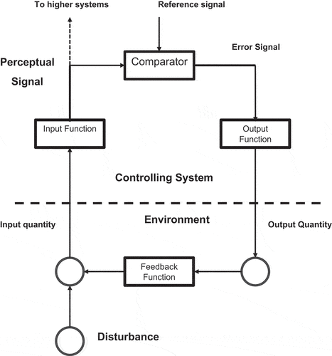
Figure 1. Perceptual Control Model (adapted from W.T. Powers et al., 2012).

Marken and Horth (2011) define the rival theories of behaviour, where sensory input causes behaviour in terms of “open loop” causality whereas PCT generates “closed loop” causality. They used results of computer experiments to support a closed loop explanation. In the case of open loop control, they claimed the output (behaviour) results from mental processing acting on the desired input.

In Figure 1 (W.T. Powers et al., 2012) the PCT model is divided into two regions; the lower half relating to the environment while the upper half represents the perception of input. Sensors detect a measure of the variable, and the organism (person) forms a perception of the value of that variable. This perception is compared with a goal or reference value obtained internally. The error that is detected drives an output such as a muscle movement that produces action to affect the variable. The environment imposes disturbances on the variable as well as that due to the organism’s action. PCT has been extended by incorporating the theory of levels to explain whole organism behaviour (P.J. Runkel, 2003).

Mansell and Carey (2015) put forward some key predictions for PCT models:

1. “If perceptual input can be controlled at a fixed value through dynamic action, then, in contrast to the stimulus-compute-response model, there will be no reliable statistical relationship between input and output.

2. Which perceptual variable is being controlled can be discovered by disturbing the perceptual input in various ways and observing which actions are produced (test of the controlled variable)?

3. Computer models based on PCT can be constructed that match the behaviour of a particular individual engaging in a real world task.”

PCT has been applied not just to psychiatry but also to education and business practice (Mansell & Carey, 2015; Forssell, 2016). Soldani (2016) provides practical applications of PCT to practical business operations in large corporations.

1.2. The Beer Game

The Beer Game devised by John Sterman (1992) at MIT was originally introduced as a board game but is now available in several internet versions (Day & Kumar, 2010; Jacobs, 2000). It has been widely used in management education across the world from the 1990ʹs to the present as a management “Flight Simulator” to illustrate how supply chains function. The Beer Game represents a simplified production–distribution supply chain system with four levels: Factory, Distributor, Wholesaler and Retailer (Figure 2). It is played by a set of 4 teams each acting as one level of the supply chain. In the basic game each level acts independently, there is no sharing of any information between levels. For reference “upstream” is defined as being the direction from any level towards the manufacturing level; and “downstream” as being the direction from any level towards the final customer. Inter-level communication consists solely of receiving orders for products from the immediate “downstream” level and shipping the orders “downstream”; and giving orders to the upstream level and receiving the ordered product from the upstream level in accordance with the inter level delay times, which are built into the operating procedure of the game (Joshi, 2000).The feedback arises from information about required demands provided at each round of play.

Figure 2. Schematic of supply chain as used by the Beer Game.

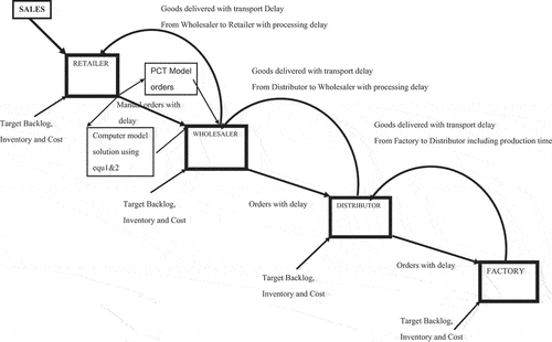
Lack of visibility of information has been demonstrated in demand and inventory amplification, which increase while moving towards the upstream level(s) (Hwarng & Xie, 2008). The game has been used to test different strategies for inventory control, for example Chen and Samroengraja (2000). The structure of the model is the same for the solely mathematical formulation; the human controlled version and the simulation proposed here using the PCT model of human decision. This is illustrated pictorially for one stage as an example in Figure 2 but was applied in all stages.

Observations by previous researchers during Beer Game activities include:

1. Individuals/groups are generally unable to allow for process delays (Diehl & Sterman, 1995; Sterman, 1989b).

2. Groups largely ignored the supply line. (Diehl & Sterman, 1995).

3. Misperceptions of feedback not only result in suboptimal performance but often lead to strategies and decision making that are contrary to optimal decisions. (Sterman, 1989a, 1989b; Paich and Sterman 1992).

4. Group performance deteriorates as delays and feedback strength become larger. (Diehl & Sterman, 1995).

Item 4, the effect of delay times on player performance was not assessed in the experiments described in this research.

Several investigators (Diehl & Sterman, 1995; Paich & Sterman, 1992; Powers, 1989; Sterman, 1987) have observed that students playing the game report feeling unable to control the situation. Sterman (1992) reported that “The game creates a real organization, with intra level ‘teams’ supposed to work together. Yet the pressures of events and the limited mental models of the players quickly cause group cohesion to break down. The game provides a vivid experience of a complex system, where players can see how the collective results of individual apparently sensible decisions can be disastrous; where participants can see the connection between the structure of a system and the dynamics it generates”.

We did not explore the intra-group dynamics and could not therefore determine how decisions are made by individuals within a group; the decisions we see are thus ascribed to the group as a single entity.

Investigators, Sterman, Deihl and Paich, have found that participants do not operate an optimal or even close to optimal ordering strategy, as defined by minimum cost, nor seem to be able to understand the supply line. Substantial research has identified chaotic behaviour in supply chains represented by the game (Mosekilde & Laugesen, 2007). Nienhaus et al. (2006) claim that panic sometimes grips the players. However, there is some evidence that younger players are less damaging to system behaviour than older players (Turner et al., 2017). The work of Alfieri and Zotteri (2017) indicates a knowledge of inventory theory does help students to operate the Beer Game. However almost all authors describing Beer Game results agree that groups perform poorly in controlling the supply line. Purvanova and Meyer (2013) have investigated the effect of personality on Beer Game performance and found that personality does affect performance, particularly for the wholesaler and distributor roles. Extroverts underweighted supply line inventory and their ordering behaviour correlated with demand amplification and extra costs. Generally, the players perform worse than the computer models of the game.

The theoretical analysis of the Beer Game is given by Sterman (2015). The order rate is defined by the smoothed demand, a measure of the supply line, SL, (on-order inventory) and the on-hand inventory, INV, with α the fraction of perceived inventory discrepancy ordered each week, the forecasting update time, θ, the fraction of unfulfilled orders each week β and the desired stock on-hand and on-order inventory, INV^’ as shown in equation 1(1) $O{R}_t=MAX\left(0,D{e}_t^e+\alpha \left(IN{V}^{\prime }-\left(IN{V}_t+\beta S{L}_t\right)\right)\right)$(1) for the order rate at time t:

(1) $O{R}_t=MAX\left(0,D{e}_t^e+\alpha \left(IN{V}^{\prime }-\left(IN{V}_t+\beta S{L}_t\right)\right)\right)$(1)

(2) $D{e}^e=\frac{z\theta }{\left(z-\left(1-\theta \right)\right)}De$(2)

The average weight on the supply line was only 34% and the players reacted aggressively to inventory shortfalls. The optimum performance by judging the cost can be calculated from these equations. This mechanisation of orders is the only difference to the human controlled Beer Game. The PCT model does not use this formulation.

This team performance problem provides the prime motivation for testing the PCT model to see if this disparity can be explained.

Naim et al. (2004) have indicated more research is needed into why the current mathematical models, mostly based on control theory, do not match actual supply chain management by humans as indicated in the Beer Game. We are proposing the use of the PCT model to provide the orders in the process in order to explain player behaviour in the Beer Game.

1.3. Review of simulation and modelling theory

Digital simulation started in 1955 with the simulation language SELFRIDGE (Matko et al., 1992) but simulation use expanded with the development of the modelling language DYNAMO in 1958 devised by the team at Massachusetts Institute of Technology (MIT) under Forrester who used it to model Industrial Dynamics (ID). A number of other major simulation languages followed, such as MIDAS, CSSL, CSMP and ACSL using the 1967 protocol on simulation languages. These languages were overtaken by the dominance of MATLAB/Simulink in the late 1990s.

Simulation of systems behaviour can be conducted by continuous representation using the simulation languages mentioned (Matko et al., 1992; Klee, 2007), and also by discrete event simulation (DES) packages such as ARENA or WITNESS or by agent based modelling (ABM) (Bonabeau, 2002). Discrete events can also be modelled in Simulink, as in this research work.

To produce a useful simulation two processes must be undertaken by the modellers. The first, verification, deals with the problem of whether the simulation does what is expected of it, while the second validation deals with the issue of whether the model produces results that match the real world. Zeigler (1976) addressed the problem of validation with his discussion of the experimental frame dividing the whole process into a real world system, a conceptual model, a lumped analysis model and a computer model. The question then becomes under what conditions does the model apply. Kleijnen (1999) discusses validation problems in situations where no real data is available and where any available data is essentially random, highlighting possible errors in interpretation.

Pidd (2003) discusses the philosophic arguments to be understood with the likelihood of three distinct types of errors. Type I errors are where the correct hypothesis is wrongly rejected and Type II errors where an incorrect hypothesis is wrongly accepted. A Type 0 error is where the modeller is on the incorrect track altogether.

Modelling of production and inventory systems dates back to the work of Simon (1952), Tustin (1953), and Vassian (1954). Vassian introduced the use of discrete transforms to allow for a fixed time of data intervals. In 1961 Forrester introduced industrial dynamics (ID), with the production of comprehensive models of manufacturing and business systems based on studies of large companies. He used control theory representation from which he was able to show that most of the observed oscillatory behaviour of product flow and supply was caused by the structure of the system, and not due to external factors. Forrester’s book (Forrester, 1961) illustrates the use of simulation to allow an evaluation of the effectiveness of many control solutions for supply chain operation.

Towill (1982), using simplified linear control theoretic models, devised an analytical solution to the problem of inventory operation, whilst retaining the overall SD form of the problem with simple management decisions such as order-up-to represented as control theory functions. Pidd (1998) and Sterman (2000, 2015) extended SD analysis to many aspects of managerial behaviour within organisations using simulation and other techniques. Kleijnen (2005) explained how simulation should be used to investigate managerial problems with a case study based on mobile communications logistics using three different simulation methods. Owen et al. (2010) reviews the application of simulation to the supply chain arguing for much wider application of simulation methods to analyse problems using the range of available tools: SD, DES and ABM.

Naim et al. (2004) discussed the various approaches used in supply chain analysis including the use of the Beer Game and simulation. They point out that the computer models of how the Beer Game operates do not match actual human performance and that understanding of how good managers become better is needed. Sarimveis et al. (2008) reviewed and ranked the performance of current mathematical models, providing data on their performance including those that incorporated optimisation.

Following Mansell and Marken (2015) the research questions being investigated in this work are:

1. Whether the behaviour of the groups in the Beer Game conforms to the concepts of PCT. To do this we need to establish whether the control is closed loop or open loop.

2. Does PCT help to explain any of the observed problems with the Beer Game as presented above?

3. What type of control engineering model would best represent a group’s perceptual control-based actions for the Beer Game operation?

2. Methodology

The task (Riemer, 2008a) of the game is to produce and deliver units of beer to the external customer at the downstream end of the supply chain. In doing so, the aim of the group is rather simple: each group has to fulfil the incoming orders of beer. The retailer receives a predetermined customer external demand and places orders with the wholesaler, who sends orders to the distributor, who orders from the factory and the factory produces the beer. Hence, orders flow in the upstream direction, while deliveries flow in the downstream direction of the supply chain. An important structural aspect of the game are delays (i.e., time lags), which model real world logistics and production times. Each delivery (and production order) requires two time increments for it to be delivered to the next level. The game is played in rounds, each representing a week in real time. In each round the groups conduct the following actions:

1) Receive incoming orders,

2) Receive incoming deliveries,

3) Update play sheets (outstanding deliveries and inventory),

4) Send out deliveries, and finally

5) Decide on the amount to be ordered and issue orders.

Effectively the only decision that players in a group are able to make throughout the game is to determine the size of the order they make; everything else follows a set of fixed rules. The first rule is that every order has to be fulfilled, either directly (if the inventory is large enough) or later in subsequent rounds. In the latter case, players have to keep track of their backlog (backorders). Secondly, inventory and backlog incur a cost – each item held in stock is costed at EUR 0.50 per week, while each item on order backlog is costed at EUR 1.00 per week. Each group is instructed to minimise their costs.

Only the retailer knows the external demand. Moreover, the game incorporates the simplification of unlimited capacity (in stock holding, production and transportation) and unlimited supply of any raw materials at the production site. In playing the game the external demand is predetermined and usually does not vary greatly. In the beginning, the supply chain is pre-stocked with inventory levels (e.g., 15 units), orders (e.g., 5 units) and beer units in the shipping delay fields (e.g., 5 units). In order to induce the bullwhip effect to the supply chain the external demand remains constant for a few rounds (e.g., 5 units for 5 rounds) before it suddenly jumps to 9 units and then it remains constant again at this higher level for the remainder of the game (usually 40 to 50 rounds in total).

The use of experimental economics, which uses controlled human experiments to investigate research and policy questions, has been justified by Croson and Donohue (2002) who state that such controlled experiments demonstrate behavioural biases that can cause empirical outcomes. A second paper by Croson (2002) sets out clearly the boundaries for testing theory, investigating anomalies and those implicit boundaries that test company policies.

A second type of experiment tests between theories and a third examines the limit of applicability of a given theory. Since we are testing the validity of a theory it is important to note that we cannot prove a theory but using Karl Popper’s falsification hypothesis (Popper, 1959) we can provide evidence for either a refutation or support for a given theory. In this paper the selection pool of subjects is that which was available, and no specific selections were made, and the published data (Reimer, 2008b), is historical.

The procedures used conformed to the protocol for research in this area of control theory as listed by P. J Runkel (1990). This protocol is set out as 9 empirical actions:

1. “Select a variable that you think the person might be maintaining at some level. In other words, guess at an input quantity – –

2. Predict what would happen if the person is not maintaining the variable at a preferred level.

3. Apply various amounts and directions of disturbance directly to the variable

4. Measure the effects of the disturbances.

5. If the effects are what you predicted under the assumption that the person is not acting to control the variable stop here – you guessed wrong about the variable

6. If an actual effect is smaller than the predicted effect, look for what the person is doing to oppose the disturbance – you may have found the feedback function

7. Look for the way the person can sense the variable. If you can find no way in which the person could sense that variable, the input quantity, stop. People cannot control what they cannot sense.

8. If you find a means of sensing, block it so that the person cannot now sense the variable. If the disturbance continues to be opposed, you have not found the right sensor. If you cannot find a sensor stop. Make another guess at the input variable.

9. If all the preceding steps are passed, then you have found the input variable the person is controlling.”

In our experimental procedure, we apply these principles to each small group, not an individual. Since data from a normally operated Beer Game was used in both data sets the choices of what actions to take were limited so that for example, protocol item 8 could not be used in this case. We first established which was the variable being controlled by evaluating the correlation coefficient between the disturbance and each of the possible variables, selected in turn as in protocol items 1–4. The variables could be, for example, the orders sent by a particular group or their backlog of orders or the cost accumulated in that level. The value of the correlation coefficient dictated whether a basic order or two stage model would be required. For most groups, the controlled input variable was the orders passed to the next stage. The choice of possible disturbance was also tested by the same process for a number of alternatives.

Test 7 was dictated by the rules of the game. The only information available to each group was the amount of beer supplied to them and the orders for beer from the group downstream. Whether the control exercised was of open loop or closed loop form was also examined (as discussed later). Only then was a suitable PCT model built and simulated to see if the real output data could be matched to that produced by the simulation using the data from the real Beer Game as inputs to the PCT model as for the human operators. The PCT model was used to substitute for the human decisions at each level and the rest of the Beer Game with attendant delays was the same as in the manual game since we used data from the manual game as inputs to the PCT model. The PCT model parameters were modified until the best agreement was obtained between the model output and the real data of each level under consideration. If a particular model structure consistently produced a low value (<0.4) of correlation coefficient between model output and real data, then a different model structure was assessed until a significantly larger correlation coefficient was obtained.

2.1. Data sources

Data used to investigate the proposed model was derived from two sources.

Data from a publicly available web site (www.BeerGame.org) (Riemer 2008b) and data generated by MSc Engineering Management students, playing the Beer Game under classroom conditions. The Beer Game was already in use as a coursework exercise in a module of their MSc programme.

In accordance with University ethical guidelines this performance data was used without the students being aware of the prospective use of the data they were generating until after the game was played. This is most important as the students should not be aware that they were on trial as this could skew the system and observations.

The student activity of playing the beer game, is an assessed piece of coursework. Therefore, practical and ethical constraints do not allow us to make significant variations in the experimental parameters, so the analysis is always post hoc. The availability of a public set of data of other groups playing the beer game was incredibly fortuitous as it provided another independent valid data set which could be used to assess our models.

To be clear both the Reimer results and the MSc results were generated by normal play in accordance with the listed procedure on the Beer Game website (https://beergame.org). The data generated was used completely independently of the players. The Beer Game data was just a source to examine the human model.

The length of the run of the game was 40 weeks for the Riemer data but the Middlesex students were limited by timetable constraints to between 12 and 20 weeks. In the US financial incentives were used with teams playing the Beer Game to provide realism to the exercise but this was not permitted for our students. From consideration of the data sources, no bias is likely due to the analysis team. The data from the MDX students was internally verified by the supervisor for completeness and accuracy of records, only one group’s data was rejected due to internal recording inconsistencies, where records of that group did not match the data from other groups. All other data obtained is included and results quoted even where the support for the thesis is not made.

The MSc students used the Beer Game spreadsheet, instructions and notes obtained from the Beer Game.org website. In the normal operation, groups recorded their choices of orders and deliveries. Students operated in groups of 3 in each of the 4 levels in the chain. The students were randomly assigned to teams and target demands were randomly assigned to each retail group as per the guidelines obtained from the website. We have found from many years of operating the game that pedagogical issues dictate that more than three students in a group led to at least one student not contributing fully. Some groups had only 2 students due to absence through illness. The number of groups was dictated by the class size.

It was not possible to vary the size of the groups during the exercise due to class time constraints.

Students were instructed to eliminate backorders and minimise costs. In order to record the data at the same time step the students used a spreadsheet to list the orders submitted and deliveries received. Students sent their spreadsheet records to the class supervisor after the game had ended. Student results were anonymised by the class supervisor (in accordance with university ethics committee protocol), and only then passed to the other authors for analysis. Many trial choices in controlled variable and disturbance were examined as in Runkel trial 1. We found that the most likely disturbance and controlled variable judged by a high correlation coefficient between the difference between the group orders and what was received defining the disturbance and the order requested as the controlled variable. This is what the group actually sees, if for example, they order 10 but receive only 8 the disturbance is −2 units.

To put the simulation process into the context of other researchers, Zeigler (1976) for example, the real world is the Beer Game arena for which the model will apply, but only for the limited range of inputs used, that of a step change in demand. It will not be validated (if it can be) for other types of input such as random demands. The conceptual model would be that described in Figure 1 and the lumped series models those described in the following section and Table 6. The computer model is the Simulink model, and this was verified to be a credible implementation of the models in Table 6 by matching final and initial values.

2.2. How does this method compare with current research?

Zhong et al. (2016) discuss the possibilities for using Big Data in supply chain management showing the huge amount of data that is now available. It is quite conceivable that this data could be used to obtain the effective input and output gains for the PCT model with a greater statistical significance, if you had access to this data. This would probably not be granted unless you have proof of concept, which this paper would provide a basis. Cho et al. (2012) use a fuzzy implementation of a service supply chain. Fuzzy control (Censlive & White, 2005) of supply chains has merit for automated implementation of ordering decisions but to explain human decisions, it lacks the necessary interpretation of actions compared with that used here with delays and system gains. Celik and Son (2010) used a sophisticated resampling routine to make state estimates of system parameters, although there are other methods extant Celik and Son’s method appears to be more efficient. The method they used would be pertinent if the Big Data mentioned above was available but would seem to give problems with samples as small as those discussed here. Celik et al. (2010) uses a different method to tune a simulation model with the DDDAS paradigm. This method was used to design a real time discrete modelling simulation to match a changing semiconductor production system. It can in principle be used to match any simulation model to real results and could be used in this problem. Because it appears to need a grid computing system, we would not be able to implement it here. Our data does not need to be evaluated in real time and these advantages may not justify the cost. The optimal system coefficient methods used by Bendavid et al. (2017), Li et al. (2016), Kouvelis and Zhao (2012), and Buzacott and Zhang (2004), for example, examining the problem of finance constrained inventory are not relevant here since we need to ascertain the fit of the PCT model to real data when we surmise the human operation will not be optimal or even be a correct model. They are designed to obtain the best solution to a constrained supply chain problem, whereas we are attempting to obtain the best model to represent the human operation.

Methods above that are in current use to research supply chains are either not applicable to investigate whether the PCT model represents real data or could not be implemented for resource reasons.

2.3. PCT models

There is no direct relationship between Beer Game and the PCT models except that the data presented to the human players in the course of playing the game is input to the PCT models. The PCT models represent the players perception of the state of the level under consideration as generated by the game. The model produces the actions of the players, in response to the perceived state of the game and the player action to achieve the perceived aim of the game.

The basic PTC model structure was derived from the work of W.T. Powers et al. (2012). The prime assumption in the qualitative PCT model is that the perceived input signal is compared to a reference set internally as in Figure 1. This input perception is governed by the disturbance. Secondary assumptions are that the input and outputs are scaled by time influenced parameters and that these can be measured.

Variables are defined in the nomenclature and the relationships can be evaluated as follows from Figure 1:

(3) $\mathbf{p}\mathbf{=}\mathbf{k}\mathbf{i}\mathbf{\ast }\mathbf{q}\mathbf{i}$(3)

(4) $\mathbf{e}\mathbf{=}\mathbf{r}\mathbf{-}\mathbf{p}$(4)

(5) $\mathbf{q}\mathbf{o}\mathbf{=}\mathbf{k}\mathbf{o}\mathbf{\ast }\mathbf{e}$(5)

(6) $\mathbf{q}\mathbf{i}\mathbf{=}\mathbf{k}\mathbf{f}\mathbf{\ast }\mathbf{q}\mathbf{o}\mathbf{+}\mathbf{k}\mathbf{d}\mathbf{\ast }\mathbf{D}$(6)

Substituting and collecting terms, where $\mathbf{G}\mathbf{=}\mathbf{k}\mathbf{o}\mathbf{\ast }\mathbf{k}\mathbf{i}\mathbf{\ast }\mathbf{k}\mathbf{f}$, the open loop gain

Hence equation 5(5) $\mathbf{q}\mathbf{o}\mathbf{=}\mathbf{k}\mathbf{o}\mathbf{\ast }\mathbf{e}$(5) for the output becomes

(7) $\mathbf{q}\mathbf{o}\mathbf{=}\left(\frac{\mathbf{G}}{\mathbf{1}\mathbf{+}\mathbf{G}}\right)\mathbf{\ast }\frac{\mathbf{r}}{\left(\mathbf{k}\mathbf{i}\mathbf{\ast }\mathbf{k}\mathbf{f}\right)}\mathbf{-}\left(\frac{\mathbf{G}}{\mathbf{1}\mathbf{+}\mathbf{G}}\right)\mathbf{\ast }\left(\frac{\mathbf{k}\mathbf{d}}{\mathbf{k}\mathbf{f}}\right)\mathbf{\ast }\mathbf{D}$(7)

Leading to the control of perception equations

(8) $\mathbf{p}\mathbf{=}\frac{\mathbf{G}}{\mathbf{(}\mathbf{1}\mathbf{+}\mathbf{G}\mathbf{)}}\mathbf{\ast }\mathbf{r}\mathbf{+}\frac{\mathbf{k}\mathbf{i}\mathbf{\ast }\mathbf{k}\mathbf{d}}{\left(\mathbf{1}\mathbf{+}\mathbf{G}\right)}\mathbf{\ast }\mathbf{D}$(8)

(9) $\mathbf{q}\mathbf{i}\mathbf{=}\left(\frac{\mathbf{G}}{\mathbf{1}\mathbf{+}\mathbf{G}}\right)\mathbf{\ast }\frac{\mathbf{r}}{\mathbf{k}\mathbf{i}}\mathbf{+}\left(\frac{\mathbf{k}\mathbf{d}}{\mathbf{1}\mathbf{+}\mathbf{G}}\right)\mathbf{\ast }\mathbf{D}$(9)

We can obtain the incremental changes by differentiating thus

(10) $\frac{\mathrm{\partial }\mathbf{q}\mathbf{i}}{\mathrm{\partial }\mathbf{q}\mathbf{o}}\mathbf{=}\mathbf{k}\mathbf{f}\mathbf{,}\frac{\mathrm{\partial }\mathbf{q}\mathbf{i}}{\mathrm{\partial }\mathbf{D}}\mathbf{=}\frac{\mathbf{k}\mathbf{d}}{\mathbf{1}\mathbf{+}\mathbf{G}}\mathbf{,}\frac{\mathrm{\partial }\mathbf{q}\mathbf{i}}{\mathrm{\partial }\mathbf{r}}\mathbf{=}\frac{\mathbf{G}}{\left(\mathbf{1}\mathbf{+}\mathbf{G}\right)\mathbf{\ast }\mathbf{k}\mathbf{i}}$(10)

(11) $\frac{\mathrm{\partial }\mathbf{q}\mathbf{o}}{\mathrm{\partial }\mathbf{D}}\mathbf{=}\frac{\mathbf{-}\mathbf{G}}{\mathbf{1}\mathbf{+}\mathbf{G}}\mathbf{\ast }\left(\frac{\mathbf{k}\mathbf{d}}{\mathbf{k}\mathbf{f}}\right)$(11)

To answer research question i) we analyse the possibility of closed loop operation as Mansell (2018) makes 4 propositions listed in Table 2. Propositions A, B and D are obtained from equation 10(10) $\frac{\mathrm{\partial }\mathbf{q}\mathbf{i}}{\mathrm{\partial }\mathbf{q}\mathbf{o}}\mathbf{=}\mathbf{k}\mathbf{f}\mathbf{,}\frac{\mathrm{\partial }\mathbf{q}\mathbf{i}}{\mathrm{\partial }\mathbf{D}}\mathbf{=}\frac{\mathbf{k}\mathbf{d}}{\mathbf{1}\mathbf{+}\mathbf{G}}\mathbf{,}\frac{\mathrm{\partial }\mathbf{q}\mathbf{i}}{\mathrm{\partial }\mathbf{r}}\mathbf{=}\frac{\mathbf{G}}{\left(\mathbf{1}\mathbf{+}\mathbf{G}\right)\mathbf{\ast }\mathbf{k}\mathbf{i}}$(10) ; C is obtained from equation 11(11) $\frac{\mathrm{\partial }\mathbf{q}\mathbf{o}}{\mathrm{\partial }\mathbf{D}}\mathbf{=}\frac{\mathbf{-}\mathbf{G}}{\mathbf{1}\mathbf{+}\mathbf{G}}\mathbf{\ast }\left(\frac{\mathbf{k}\mathbf{d}}{\mathbf{k}\mathbf{f}}\right)$(11) . If G is large and positive A tends to zero for a closed loop. B tends to 1/kf, low to zero. C is large and negative and D less than 1 but positive.

Table 2. Correlation between variables for open and closed loop (from Mansell, 2018).

Proposition to support closed loop/ open loop choice	Relationship between variables	Open Loop	Closed loop (PCT)
A	D & qi	High positive	Low to zero
B	qi & qo	High positive	Low to zero
C	qo & D	High positive	High negative
D	qi & r	N/A	High positive

To move from a qualitative PCT model to a quantitative model we used the rationale and elements (Table 1), common to SD since Forrester (1961) maintains that ALL systems can be described by these elements; stocks; rates; loops; delays and other simple processes. The observation of Forrester was that the simplest view of decision processes was an amplification or attenuation of the information signal and a simple time delay. The use of this SD method has been shown to apply quite universally (Sterman, 2000). Although the input and output blocks in Figure 1 can be mathematically represented in different formulations, we found that the gain and exponential delay representation was the simplest that was compatible with the data from the Beer Game and therefore using Occam’s razor was the representation chosen to be modelled.

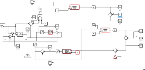
PCT models (Table 6) used in the simulations were of two basic schemes; those denoted O# based on the order level only with the number indicating the number of models tested to that point, and those denoted B based on a second level perceiving backlog as well as the order level, providing extra internal input to the mind processing the problem.

To investigate research question iii) Four basic models of the human operator were tested in this work. The simplest (O3) corresponded to the formulation used by Powers et al. (2012), the input is in the form of a gain plus an exponential delay. Model O3 is an order-based model with integrator and gain in the output with 3 parameters that can be varied to optimise the performance of the model. The O3 model was used in the tracking experiments of Bourbon et al. (1990) based on measurements of operator behaviour. Integration of the output signal was observed to describe the path from error to output in their tracking experiments. All the models were implemented in MATLAB/Simulink with the most successful model (O4) shown in Figure 3. Model O4 is an order-based model with 4 parameters and an exponential delay in the output, with K1 the input gain, K2 the output gain, S the input time delay and Q the output time delay. There are two limiters to ensure that only positive numbers are output at each stage (orders cannot have a negative value). In these models (e.g., Figure 3) the data input to the model was the Demand as reference value and the Disturbance as input. This data was taken from the spreadsheet data for the manual game at each different stage and the output, orders from the model were compared with the orders generated by the human groups.

Figure 3. Simulink Order Perceived Model (OPM) denoted O4.

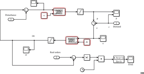
This version of the output control is different to the structure of the models tested in the tracking experiments of Bourbon et al. (1990). The input and output functions of Figure 1 are represented in the Simulink diagram Figure 3 by two discrete transfer functions that incorporate gains and time delays. This structural modification was made because the effect of the integrator in the output block was generally found to give a poor fit to the data, except in one case. It takes time to recognise a defined change has occurred and this is not represented in the model by an integrator but by a delay.

Modified models B5 & B6, Figure 4 & 5, incorporate a reference signal from the backlog to improve the fit of the model in five cases only. This model incorporates the order model as a subsystem. B5 is a Backlog model with 5 parameters while B6 is a Backlog model with 6 parameters both models including a time constant T for backlog delay. The backlog control is another delay transfer function with gain. In model B5 the gains and delay times are the same as the input stage of the order model and a fraction of the backlog is added to the error before the delay. In model B6 (Figure 5) all the 6 gains are free to be optimised. The backlog model appears to fit better when the (spreadsheet) data indicates that the control variable is the backlog as would be expected. All the models are operated using Simulink discrete transfer functions as the data is discrete.

Figure 4. Backlog Control.

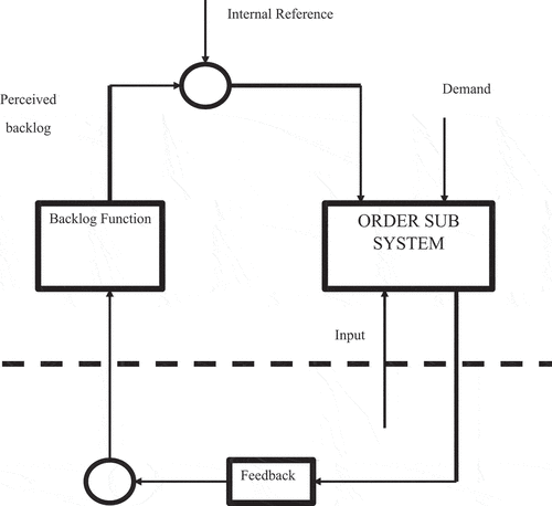
Figure 5. Simulink model of Backlog Model B6.

Research question ii) will be partly answered by what order model is needed and the overall delays and scaling of the input and output blocks in the model. If only order based models are found, then the players do not consider backlog and cost in their mental models for example.

To use the correct model, we examined the correlation coefficient of output and experimental data for various postulated control variables. If this indicated a priority in orders was the subject of control, we used an O4 model. Where the values of the correlation coefficient between the output from the model and the observed orders, was less than 0.5 then we investigated other models’ structures. If a control variable, such as backorders, was indicated then model B5 was initially used. Finally, if sufficient convergence to an acceptable correlation coefficient was not achieved then we tried model B6.

Previous research (Sheridan & Ferrell, 1981) into human transfer models for vehicular control used harmonic inputs and Bode analysis to verify the transfer functions including the “crossover” model (McRuer & Krendel, 1973). These measurements were made with continuous data. The reason the correlation coefficient was the first criterion used here on the limited discrete data set was a) to match previous published work on the verification of PCT in psychological experiments and b) the problem that to use sinusoidal inputs would need much longer exercises than was practicable. We made other evaluations using two control engineering weighting criteria (Ogata, 1990), the minimum Integral of Absolute Error (IAE) versus time over the whole simulation where the error,$\epsilon$ was the difference between the model output orders and the orders generated by playing the Beer Game for a particular group. These criteria are widely used in control engineering to determine the optimum response to a deterministic input (D’Souza, 1988) by varying the coefficients of the transfer function. The final value in these simulations was then used to select the minimum values of IAE and ITAE, defined in equations 12(12) $\mathrm{I}\mathrm{A}\mathrm{E}=\int \left|\epsilon \right|\mathrm{d}\mathrm{t}$(12) & 13(13) $\mathrm{I}\mathrm{T}\mathrm{A}\mathrm{E}=\int \mathrm{t}\left|\epsilon \right|\mathrm{d}\mathrm{t}$(13) , by using a range of K1, K2, S and Q quantities.

(12) $\mathrm{I}\mathrm{A}\mathrm{E}=\int \left|\epsilon \right|\mathrm{d}\mathrm{t}$(12)

(13) $\mathrm{I}\mathrm{T}\mathrm{A}\mathrm{E}=\int \mathrm{t}\left|\epsilon \right|\mathrm{d}\mathrm{t}$(13)

3. Results

Data for each group showing the standard deviation of orders data is given in Table 3. It can be seen that for the Riemer data (Reimer, 2008b), spread of values of standard deviation of orders increases from the retailer level upstream to the factory level illustrating the bullwhip effect (Sterman, 2000). With the exception of the Middlesex distributor groups this is also true of values of the order standard deviation for the other groups. However, two of the Middlesex groups show very large variation, more than three times the least, compared to their fellows at the same level. The distributor groups, in particular, show a very large variation in orders. If we exclude groups with large variations in standard deviation as noted above and select pairs of values from corresponding Riemer and MDX student groups and apply a Kolmogorov-Smirnov 2 sample test; the results, indicate that the two data sets are essentially from the same continuous distribution with 95% confidence level against the null hypothesis that the data are not from the same continuous distribution. Two MDX groups and one Reimer group have low correlation coefficients and can be considered not to support the PCT model.

Table 3. Standard Deviation of orders, for each round, for different groups (R = Reimer group, M = Middlesex group).

Group	Rr1	Rr2	Mr1	Mr2	Mr3	Mr4	AV	Rw	Mw1	Mw2	Mw3	Mw4	Av	Rd	Md1	Md2	Md3	AV	Rf	Mf1	Mf2	Mf3	Mf4	AV
Retailer	7.61	3.92	5.84	5.22	17.52	5.16	8.4
Wholesaler								8.42	6.89	22.1	5.84	13.0	12
Distributor														15.4	47.5	53.8	24.3	41.9
Factory																			17.4	5.95	47.4	9.5	19.8	18.2

The first part of the investigation assessed whether a closed loop solution was supported. The propositions stated in Mansell (2018) can be examined with respect to the equations shown above. This proposition indicates the correlation to be expected between the variables when a high loop gain G is present from equations 3(3) $\mathbf{p}\mathbf{=}\mathbf{k}\mathbf{i}\mathbf{\ast }\mathbf{q}\mathbf{i}$(3) –11(11) $\frac{\mathrm{\partial }\mathbf{q}\mathbf{o}}{\mathrm{\partial }\mathbf{D}}\mathbf{=}\frac{\mathbf{-}\mathbf{G}}{\mathbf{1}\mathbf{+}\mathbf{G}}\mathbf{\ast }\left(\frac{\mathbf{k}\mathbf{d}}{\mathbf{k}\mathbf{f}}\right)$(11) . This is true for proposition A. If there is not a high loop gain then the best value here would be around 0.5, but still positive. For proposition B, the relationship between qi & qo is not correct since the value is equal to kf, which is likely to be 1. The most important closed loop criterion is proposition C which is true for high loop gain. For proposition D this is true for high loop gain and for low gain the value is still positive. Using the Beer Game data from groups as shown in Table 4 it can be seen that proposition C is strongly supported but proposition A is not. Proposition B is supported; hence no open loop solution and proposition D shows that the loop gain is small. The data therefore supports a closed loop system of small loop gain.

Table 4. Riemer Data Spreadsheet Correlation coefficients of parameter data to projected disturbances.

Retailer	Orders	Backlog	Demand	Cost
1	−0.71	−0.26	−0.16	−0.19
2	−0.61	−0.17	−0.03	−0.29
Wholesaler	−0.62	−0.15	−0.03	0.11
Distributor	−0.78	−0.29	−0.12	−0.15
Factory	−0.74	−0.36	−0.18	−0.05

The disturbance or environmental effects are registered by each group as the difference between the order they make on their upstream supplier and the quantity they receive as a delivery. The reference level they have for their internal model is the order they receive from their downstream level. As discussed in section 3, it was required to identify which variable was the subject of control. From most group results this is clearly the orders sent to the next level upstream. This is shown in Tables 4 & 5. Correlation coefficients of different variables and the disturbance have been calculated using a spreadsheet (Table 7). For the orders to the upstream level the correlation coefficients vary between 0.43 and 0.8, with 60% of the group orders exceeding 0.7 at a confidence level of 95%. Two of the lower values, for MR1 & MR2, have spreadsheet correlations with backlog that could not be evaluated as the backlog was maintained at zero. The participants were generally not controlling the backlog or the cost in the system as instructed. Whilst values of correlation coefficients as high as those reported, >0.9 for the experiments in tracking (Bourbon et al., 1990), were not obtained, the values found in this study are considered statistically significant in each case.

Table 5. Sample correlation between different variables (Riemer data).

Group	Prop C D2qo	Prop B qi2qo	Prop A D2qi	Prop D qi2r
Retailer	−0.708	−0.2	0.833	0.1
Wholesaler	−0.62	−0.067	0.74	0.16
Distributor	−0.78	0.12	0.53	0.09
Factory	−0.74	0.27	0.45	0.33

Table 6. Model representation.

MODEL	Input Function	Output Function	Backlog Function	Backlog Gain
O3	$\frac{K1\ast \mathrm{z}}{\mathrm{S}\ast \mathrm{z}+(1-\mathrm{S})}$	$\frac{K2\ast \mathrm{z}}{\mathrm{z}-1}$
O4	$\frac{K1\ast \mathrm{z}}{\mathrm{S}\ast \mathrm{z}+(1-\mathrm{S})}$	$\frac{K2\ast \mathrm{z}}{\mathrm{Q}\ast \mathrm{z}+(1-\mathrm{Q})}$
B4	$\frac{K1\ast \mathrm{z}}{\mathrm{S}\ast \mathrm{z}+(1-\mathrm{S})}$	$\frac{K2\ast \mathrm{z}}{\mathrm{Q}\ast \mathrm{z}+(1-\mathrm{Q})}$	$\frac{K1\ast \mathrm{z}}{\mathrm{S}\ast \mathrm{z}+(1-\mathrm{S})}$	$K3$
B5	$\frac{K2\ast \mathrm{z}}{\mathrm{Q}\ast \mathrm{z}+(1-\mathrm{Q})}$	$\frac{K3\ast \mathrm{z}}{\mathrm{T}\ast \mathrm{z}+(1-\mathrm{T})}$	$\frac{K1\ast \mathrm{z}}{\mathrm{S}\ast \mathrm{z}+(1-\mathrm{S})}$	$K3$
B6	$\frac{K2\ast \mathrm{z}}{\mathrm{Q}\ast \mathrm{z}+(1-\mathrm{Q})}$	$\frac{K3\ast \mathrm{z}}{\mathrm{T}\ast \mathrm{z}+(1-\mathrm{T})}$	$\frac{K1\ast \mathrm{z}}{\mathrm{S}\ast \mathrm{z}+(1-\mathrm{S})}$	$K4$

Table 7. Correlation coefficients for MDX data.

Test	Length of run	Team				Spreadsheet Correlation coefficient with disturbance			Correlation Coefficient
Date	Simulated weeks	Retailer	Wholesaler	Distributor	Factory	Orders	Backlog	Demand	with model
5/12/19	21	1				−0.79	na	−0.28	O4	−0.54
5/12/19	21	2				−0.79	na	−0.13	O4	−0.65
27/11/19	23	3				−0.74	0.05	−0.4	O4	−0.66
4/12/19	12	4				−0.59	−0.45	0.58	B5	−0.73
4/12/19	13		1			−0.88	−0.33	−0.22	O4	−0.74
27/11/19	23		2			−0.43	−0.57	−0.23	B5	−0.75
5/12/19	20		3			−0.75	−0.29	−0.26	O4	−0.69
5/12/19	21		4			−0.79	−0.38	−0.36	O4	−0.72
27/11/19	22			1		−0.77	−0.66	−0.33	O4	−0.64
4/12/20	13			2		−0.2	−0.32	−0.5	O4	−0.84
4/12/19	12			3		−0.95	−0.73	−0.62	O4	−0.78
5/12/19	20				1	−0.58	−0.68	−0.58	B5	−0.63
27/11/19	24				2	−0.72	−0.23	−0.28	O3	−0.44
4/12/19	11				3	−0.74	0.64	0.41	O4	−0.74
5/12/19	22				4	−0.72	−0.06	0.41	O4	−0.81

Testing the significance of correlation

We formulate a null hypothesis that the data sets are uncorrelated. The test is two tailed using the test equation from Lind et al. (2000)

(14) $\mathrm{t}=\frac{\mathrm{r}\sqrt{\mathrm{n}-2}}{\sqrt{1-{\mathrm{r}}^2}}$(14)

with n-2 degree of freedom.

If we choose a level of significance of 0.05 (95% probability) and use as an example data from MDX group D1 in Table 6, n is the number of data points 22.

This yields a t value, from equation 14(14) $\mathrm{t}=\frac{\mathrm{r}\sqrt{\mathrm{n}-2}}{\sqrt{1-{\mathrm{r}}^2}}$(14) , of 8.46 for orders and a t value of 1.56 for demand. The decision rule from the Student t distribution states that if the computed value of t lies between −1.725 and +1.725 the null hypothesis is not rejected. For the order correlation this is not the case, and a correlation exists between the perceived disturbance and the orders received. This not the case for the demand and the assumption of correlation is rejected. The underlying assumption of equation 14(14) $\mathrm{t}=\frac{\mathrm{r}\sqrt{\mathrm{n}-2}}{\sqrt{1-{\mathrm{r}}^2}}$(14) is that a linear relationship exists between the variables. A zero value of correlation coefficient does not preclude a non-linear relationship between the variables.

The largest correlation coefficients between the model response and real Beer Game data obtained by parameter variation are all greater than 0.44 as shown in Table 8. The nearer the correlation coefficient is to a modulus of 1 the closer is the match obtained between the model response and the real data. This Table for all groups contains the coefficients for the model parameters, the correlation coefficients and the probability of random association. For the majority, the correlation is in excess of 0.7 and for this quantity of data this value represents a significant degree of correlation. Only in five cases out of 20 is the best data fit model different from the basic order model PC Theory implementation (O4). Sample plots of experimental data versus the model outputs are shown in Figure 6. These plotted comparisons are indicative of good agreement between model performance and experimental data. Figure 7 indicates how the values of system constants we obtained for the O4 model varied across the supply chain levels. The values for K1 are consistent with a value of 1.1 for all levels. This implies a similar recognition gain. The values for K2, the output gain, are clearly less for each level the further it is from the customer. This is what we would expect as the retailer needs to respond sharply to demand, while the other levels have more time to respond. The two time constants do not vary much from values of 1.5 weeks. This implies similar reaction times for all levels but the value of output time constant Q for the retailer is longer which may explain why the gain is larger.

Figure 6. Riemer distributor data comparison CC = −0.71.

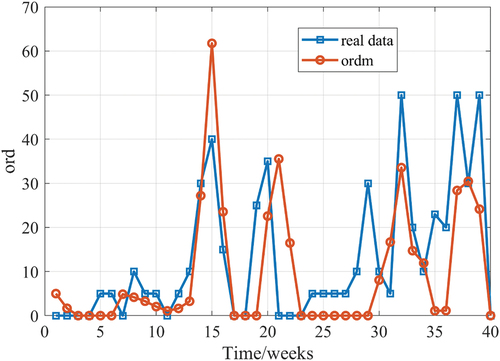
Figure 7. O4 model constants for different levels.

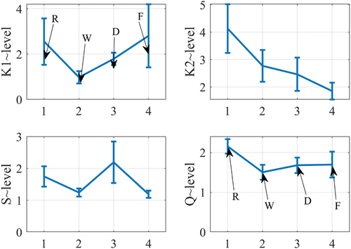
Table 8. Largest values of Group Correlation Coefficients and Model Parameters.

Grp	CC	K1	K2	K3	K4	S	Q	T	Probability P
	Riemer data set 1
RR11	0.68	2.085	3.97	1.38		2.01	0.7		1.5e-6
RW	0.77	0.25	3.05			1.36	1.55		5.7e-8
RD	0.71	1.1	1.5			2.3	1.1		1.8e-7
RF	0.76	0.02	2.05			1.05	1.05		1.6e-8
	Riemer Data set 2
Grp	CC	K1	K2	K3	K4	S	Q	T
RR2	0.67	6.97	6.77	2.25	1.8	1.68	2.58	0.72	0.0001
	Middlesex Data
Grp	CC	K1	K2	K3	K4	S	Q	T
MR 1	0.54	2.15	4.1			2.34	2.15		0.01
MR 2	0.65	0.74	2.6			1.66	2.47		0.006
MR 3	0.66	4.77	5.69			1.24	1.84		0.0006
MR 4	0.73	0.34	5.1	3.95		0.67	2.92		0.007
MW 1	0.74	1.25	1.15			1.5	2.01		0.004
MW 2	0.75	0.29	1.42	2.35		4.85	2.05		0.00004
MW 3	0.69	1.5	3.9			1.185	1.225		0.0007
MW 4	0.72	0.9	2.97			0.91	1.22		0.0003
MD 1	0.64	1.6	3.25			1.22	1.81		0.001
MD 2	0.84	2.65	3.75			1.25	1.95		0.0003
MD 3	0.78	1.8	1.35			4.0	1.85		0.0003
MF 1	0.63	5.65	2.98	3.63		4.19	4.12		0.003
MF 2	0.44	1.01	1.14			0.29			0.03
MF 3	0.74	4.35	2.25			1.41	1.93		0.009
MF 4	0.81	4.05	1.25			1.1	2.1		0.00001

The correlation coefficients for the match between the PCT simulation and the MDX student results, were computed in MATLAB 2018b using the “corrcoeff function” which tests “the hypothesis of no correlation against the alternative that there is a non-zero correlation. The value of percentage probability P for n measurements of the two data sets of uncorrelated, model predictions” of orders and the real orders, giving a correlation coefficient (CC) greater than a set value say 0.5, in the Riemer data case where n = 40 is 0.1% (from J. R. Taylor, 1997). Since all the Riemer data correlation coefficients are greater than 0.67 the probability of two such sets of data randomly producing such a large correlation coefficient is less than 0.05%. Hence, we can say the correlation between model generated data and the experimental observed data is statistically significant at the 95 % level.

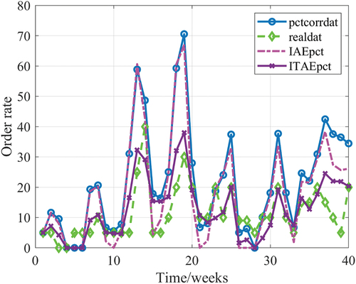
Figure 8 illustrates how the real data compares using the PCT model with three sets of constants. In this case the ITAE constants give the closest agreement.

Figure 8. PC constants from three methods in comparison to Reimer Wholesaler data.

4. Discussion

Power’s PCT was originally applied to individuals, whereas in this present work we applied the basic theory to small groups of 2 or 3 people, with inevitable intra-group conflicts and arguments, which may cause decision delay. One reason for starting this series of tests with relatively small groups is that PCT models for larger teams need much greater complexity using levels to deal with individual to individual reactions.

Since the original psychological testing on the PCT model on individuals used correlation coefficients these were the first of the three methods of validating the models used by us. From the spreadsheet data in Table 4 the correlation coefficients greater than 0.7 between the orders and the disturbance, for the groups investigated, indicated a clear objective of the group trying to control the orders, not the cost or backlog as suggested in their instructions. An exception is group MD2 (Table 3) where the order correlation coefficient is 0.2, judged to be not significant, and for this group the largest correlation coefficient is with the demand from the wholesaler. Similar exceptions are occurred for groups MW2 and MF1. Despite this the O4 model has a correlation coefficient of 0.84 with the real output data for group MD2. This group clearly operated on the principle of satisfying the demand, but this meant generating a numerical order level close to the demand level, which incorporated the disturbance. In the cases where the orders were not the singular control variable; the spreadsheet data indicating control variables is split between the orders, backlog and demand for the two Riemer retail groups and three Middlesex groups MR4, MW2 and MF1.

The second research aim of the experiments was to see if the data supported a closed loop control solution. The PC website did not present any discussion about the predictions for closed loop systems. Quoted results in Table 4 are for systems with high loop gain and the implication is that a high loop gain was not present in the systems under investigation here. The model results confirm that this is the case. The principal argument for a closed loop solution is the relation of the output (orders sent) to the environmental input (disturbance), which we found to be a high value negative correlation. This is seen in all groups except MD2. The relationship between input and output is seen to be low from Table 4 supporting concepts in Mansell (2018). Our experimental data generally supports and does not contradict a human closed loop model.

A relationship, indicated by a low correlation coefficient, between input and the reference value is weak whereas the values for environmental value and input are high contrary to Table 2. Examination of equation 6(6) $\mathbf{q}\mathbf{i}\mathbf{=}\mathbf{k}\mathbf{f}\mathbf{\ast }\mathbf{q}\mathbf{o}\mathbf{+}\mathbf{k}\mathbf{d}\mathbf{\ast }\mathbf{D}$(6) shows that the correlation between,$Dandqi$ proposition A, depends on the value of $\mathrm{k}\mathrm{d}$, which in this case has a value of 1. This disagrees with Table 2.

The case for a closed loop is supported by much of the data whereas the data does not support an open loop solution.

The PCT models do not produce close agreement for the gains or time constants for the various groups as presented in Table 5. For each group, the disturbances are different, and the judgements are different. Responses are different; so, we would not expect the same response except by coincidence. The parameter ranges of K1, K2, S and Q for different length of experimental data are shown in Figure 7. In Figure 7 the data for the value of K1 the Middlesex data is self-consistent but the Riemer data range is much smaller, implying that the Riemer groups need less signal to perceive what is happening. It is not known whether the Riemer groups had prior practice playing the game or better understanding of the underlying inventory theory or a significant level of guidance before this data was produced. This is not the same for the output gain K2 where all the data is within the error range of each other. The results for S show that there is no consistent difference between results for different lengths of run. Values for Q do show quicker reaction by the Riemer players. So that the Riemer groups need less signal, lower K1, to perceive the problem but are no quicker than the Middlesex students to do so (S is not much different). Riemer groups appear quicker to react when the problem is perceived, suggesting greater experience.

The global results for the IAE optimised O4 models are: K1 = 1.94 ± 0.40; K2 = 2.7 ± 0.36; S = 1.6 ± 0.22 and Q = 1.73 ± 0.12 for the 14 data sets. The range of correlation coefficient of the model generated orders to the real observed orders is 0.70 to 0.74.

The retail level has the lowest value of correlation coefficient. Parameter values for the fitted O4 model K2, the output gain, has a downwards trend towards the factory level. Is this a reflection of the bullwhip effect? The distributions of model delay times, S and Q, for each level are consistent with the global values. We conclude that PC models designed to represent individual behaviour can also be applied to small groups (2–3). The observations of Purvanova and Meyer (2013) regarding personality effects, may well explain some of the excessive over ordering in some of the Middlesex groups i.e., a dominant individual may override the more conservative viewpoint.

It should be noted that in the numerical iteration for the optimum correlation a number of local maxima exist that give values within 20% of the value given in Table 8 and the presented searches may not have yielded the absolute greatest maximum. Several of the groups produced data that was matched by models with very long time constants far in excess of two weeks. We suggest that these groups could not make decisions within the time scale of the built in delivery delays. This surmise supports the observations in item 1 of the problems with the Beer Game, in other researcher’s findings. All the groups did not prioritise the supply line and concentrate on orders alone (item 2). Even in the implementation model only five groups’ data needed reference to the backlog to match the data. Since the constants in the fitted models vary so much, clearly many groups were operating sub-optimally again agreeing with item 3 of problems noted by researchers of the Beer Game. Since the delay times were not varied, no conclusion can be made with reference to item 4 of the Beer Game problems.

In the backlog models the gains are higher than those for the O4 model. Some of the delay times are excessive. Leading to the interpretation that the more complex the decision to be made the more delay in implementing an action as might be expected in this work where decisions are a group consensus. The only O3 model gave a low correlation coefficient of 0.44, whereas the O4 model gave a correlation coefficient of 0.42 for the same group and the B5 model gave a correlation coefficient of 0.37. These low values,<0.5, show this group was having difficulty making the best decisions and for this specific data we argue that the PCT model is not supported.

Reasonable agreement with the model’s constants is obtained between the model parameter values for maximum high correlation and those for minimum IAE or ITAE (see, Table 9). This shows that the model is in control engineering terms a good fit to the experimental data or that the efficacy of the model is confirmed. This agreement is illustrated in Figure 8 using the Reimer wholesaler data as an example. In this case the correlation coefficient and the minimum IAE data model are close, but the ITAE data model is closer to the real data. This is not true in all the cases examined but is correct for the larger number of trials. However, we judge that all the variations of PC system constants produce respecTable agreement with the real orders.

Table 9. Sample Engineering Criteria to obtain system constants.

Group	RW			RD			MW4
Constants	Max CORR	Min IAE	Min ITAE	Max CORR	Min IAE	Min ITAE	Max CORR	Min IAE	Min ITAE
K1	0.25	0.4	0.45	1.1	1.0	1.0	0.9	0.86	0.9
K2	3.05	3.0	1.7	1.5	1.55	1.5	2.97	2.1	2.1
S	1.35	1.45	1.95	2.3	2.35	2.4	0.91	0.8	1.0
Q	1.55	1.5	1.6	1.1	1.15	1.2	1.22	1.2	1.4

The two sets of data; measured orders and model predicted orders, for the best fit correlation coefficient values, were also tested using a Kolmogorov-Smirnov 2 sample test returning a null hypothesis at 95% confidence that the data in the two groups are from the same continuous Beer Game distribution.

But several of Riemer’s groups’ data could be interpreted as players having some prior familiarity with the game, whereas we know that the MSc students had no prior experience.

4.1. Management implications

If the conclusions from this investigation are generally applicable to the process of human decision making in supply chain management, then a number of observations relevant to business operations can be made. Normal operations of a supply chain may be controlled effectively but inefficiently (Sterman, 2015). Effective control can be achieved if the system is stable to demands and produces a response that satisfies certain limits. Whereas efficient control in this case is related to achieving minimum cost as well as a stable limited response.

Recognition of a change in perception takes at least three increments of information to register with the team. This means that as events change rapid information transmission is needed to enable the perception to be relevant. The clarity of objectives is perhaps the most important criterion. The behaviour of groups tested here suggested that they were unclear as to what they were trying to achieve. Training is normally considered essential for managers but the evidence for learning in larger run times is not visible.

Action times are between 1 and 2 time increments. This should be built into any control system devised by management for critical business operation. Providing operational staff with the ability to shorten this recognition time by extensive modelling of the situations in use.

Other researchers have found training does improve responses in the Beer Game. We cannot draw any conclusions on this point as it was not tested in our experiments, however length of run of the data does seem to have a small effect.

Soldani (2016) recommends the following steps based on PCT to operate teams effectively:

“Find out how a person’s perceptual system is organised. Ask the person to make a value judgment. Ask the person to make an active commitment and Cooperate with the person to make a plan to implement the necessary changes”

These procedures were found to have profound implications for the operation of individuals and teams in large US corporations.

How do the experiments reported here fit into management theories?

Current management theories can be divided into three broad groups: Scientific Management; Behavioural theories and Modern Management Practice.

Scientific management, generally attributed to origins in the work of F.W. Taylor (1911) includes the ideas of training and management ambition with worker understanding being central to efficiency. It was always assumed that mere commands would be sufficient to facilitate behaviour, which the Beer Game demonstrates is not the case. Soldani (2016) has shown PCT implies that managers cannot assume that this synchronicity of concept has happened by dictat, the other principal feature of scientific management.

Behavioural theories of management focus on style of leadership and involve considerable assumption about a person’s traits and personality. Again Soldani’s (2016) work on PCT would imply that what has been attributed to personality may just be a lack of understanding and communication on the importance of company goals.

More modern management techniques such as quantitative approaches using Management Science, Operations management and Management Information Systems rely heavily on decision theory which, as the experiments above show, are situations where there are not clear decisions due to uncertain information patterns. These management techniques may lead to more effective communication and display of information, lack of which is shown to be significant in systems failures of all kinds. Applying the Law of Variety (Ashby, 1958) requires that all workers participate in finding solutions to business problems and the lessons of PCT imply that their appreciation of the problems need to be aligned so that better communication on an individual level is needed from managers. The models generated above if replicated in larger scale experiments could be used to optimise systems in business with much greater certainty. The current theme of Service dominated logic, for example, (Lusch & Vargo, 2015), could possibly benefit from an ability to grasp how individuals actually deal with the concept of value and use the methods here to evaluate them.

5. Conclusion

Sets of Data from two distinct and independent sources have been used to investigate whether a PCT model could explain the performance of small groups of human operators controlling a manually operated Beer Game representation of a supply chain. This work was designed to see if PCT could explain published research results that showed poor human manager performance in controlling supply chains as represented by the Beer Game and to aid understanding of how human decisions were made. The PCT models represent the players perception of the state of the game and the models can then produce outputs which are functions of the inputs and decisions based on the perceived state.

A correlation coefficient greater than 0.68 at 95% probability was found for comparison of our model generated orders and pooled experimental order data for both data sets for 17 out of 20 groups where inter level orders or level backlog was the controlling variable.

There is data (Table 5) supporting the principle that closed loop control applies to the behaviour of small groups in this situation but there are some problems; principally that the choice of control variable is not unambiguous, and the groups could be trying to control several parameters at the same time but with different prioritisation.

From the results presented here there is strong support (represented by a larger correlation coefficient) for the controlled variable being the orders made to the next upstream level.

Generally, the groups’ disturbance data did not show strong correlations with backlog or cost or demand, which they were instructed to control simultaneously. This might explain the operators’ confusion in controlling the system.

Where more than just orders were being controlled the delays in decisions appear to have increased, leading to the suggestion that the groups needed extra help to cope when controlling several variables.

Simulink order-based PCT models’ responses are shown to provide a good match with experimental data on inter group orders sent upstream. Three separate mutually supportive indices, Correlation Coefficient; IAE and ITAE were used to validate the models to the real Beer Game data. The first found correlation coefficients greater than 0.63 for 18 out of the 20 groups investigated. Only in two groups did the correlation coefficient of experimental orders and model responses fall below 0.55. Five groups needed a more complex implementation of the model to achieve a good match. The second index used with two optimised ITAE and IAE criteria producing fair agreement with the model systems constants obtained from the correlation coefficients (Table 9). Third, applying a Kolmogorov-Smirnov 2 sample test at 95% probability between the experimental data and that from the Simulink model confirms the null hypothesis that the data in the two groups are from the same continuous distribution i.e., that they do agree that the model is in close agreement with the real world of Beer Game results.

The good match between model response and experimental data is achieved despite large differences in game run times for the separate groups.

For research question i); within the bounds of the analysis presented here, the answer is yes

For research question ii); the answer is supported for problem items 1 to 3 in Table 2.

For research question iii); the model O4 appears to be the best representation for these present sets of data for the majority of examples used.

In summary the research indicates

1. There is significant evidence that the behaviour of groups playing the Beer Game is better represented by closed loop human control models, rather than open-loop human control models.

2. The overall conclusion is that PCT can be applied to small (1–3 people) groups, playing the Beer Game, for the range of inputs tested, despite possible internal conflict about choice of group actions. However, this is not supported for 10–15% of the data obtained.

3. A simple PCT model can be devised, which represents with reasonable accuracy the behaviour of small groups of Beer Game players in response to their perception of the required tasks and actions from Beer Game data for the majority of cases tested. Some groups needed a more complex model to explain their behaviour, even then these results were not unequivocal.

4. Some groups exhibited slow recognition of perception and a correspondingly excessive action in response. The recommendation is to devise aids to help operators recognise the change in input variables.

5. In general, the results here support the observations made by other investigators of the Beer Game that the players do not recognise supply chain delays or backlog and we found no correlation with perception of cost.

6. It is fairly clear from these tests that operators need to be given clear instruction about priority of tasks in any management exercise. Since all current management theories rely on shared objectives to achieve company success these experiments show that even in the case of only three simple objectives, operators can be quite confused about relative priorities.

7. When teaching how to play the game, practitioners need to be helped to develop an order strategy to minimise inventory and backlog.

8. Even if the simple PCT model is not the true explanation of group behaviour it may be used as a better approximation of the decision process than current non-numerical theories.

5.1. Future Work

Repeat experiments need to be made using a much larger set of Beer Game participants to examine the efficacy of the models derived here. A number of different inputs in type and size needs to be examined to extend the range of applicability of the models.

The effects of group size and intra-group dynamics also need to be investigated.

Repeat trials should be made with the same groups to investigate any “in-game” learning effect. An investigation needs to be conducted to determine the maximum number of conflicting input criteria that a group can manage, whilst still maintaining effective control of their tasks. Work with computer operators suggests that five items can be controlled but the situation here would cast doubt on that. Correlation of the model responses to actual group activities using psychological profiling of game participants will be determined. A multiple level PCT model applied to individuals’ interactions in a group when in a situation with conflicting requirements can be produced.

Nomenclature

Table

B5	5^th model tested includes backlog feedback
B6	6^th model tested includes backlog feedback
D	the environmental disturbance
De	Demand
e	is the error perceived between the reference value and the perceived input variable
G	Transfer function
IAE	Integral of Absolute error
INV	Stock
ITAE	Integral of Time multiplied by Absolute Error
K1	input gain
K2	output gain
kd	disturbance gain
kf	feedback gain
ki	input steady state gain
ko	output steady state gain and spurious
MD	Middlesex students distributer level
MF	Middlesex factory level
MR	Middlesex retail level
MW	Middlesex wholesaler level
n	number of data points
O3	3^rd order based model tested
O4	4^th order based model tested
p	the value of the perceived variable,
PCT	Perceptual control Theory
Q	output time delay
qi	the input to the organism,
qo	the output from the organism,
RD	Reimer distributor
RF	Reimer Factory
RR	Reimer retailer
RW	Reimer Wholesaler
r	the reference value, correlation coefficient
S	input time delay/weeks
SL	Supply line
T	backlog time delay/weeks
t	time
t	Student’s t
z	discrete transform
Greek
α	Fraction of perceived inventory discrepancy
β	Fraction of supply line of unfilled orders
θ	Forecasting update time

Disclosure statement

No potential conflict of interest was reported by the authors.

References

- Alfieri, A., & Zotteri, G. (2017). Inventory theory and the Beer Game. International Journal of Logistics Research and Applications, 20(4), 381–404. https://doi.org/10.1080/13675567.2016.1243657
- Angerhofer, B., & Angelides, M. (2000), “System Dynamics modelling in supply chain management: Research a review”, Proceedings of the 2000 Winter Simulation Conference, USA. IEEE.
- Ashby, W. R. (1952). Design for a brain. Wiley & Sons.
- Ashby, W. R. (1958). Requisite variety and its implications for the control of complex systems. Cybernetica, 1(2), 83–91.
- Bendavid, I., Herer, Y. T., & Yücesan, E. (2017). Inventory management under working capital constraints. Journal of Simulation, 11(1), 62–74. https://doi.org/10.1057/s41273-016-0030-0
- Bonabeau, E. (2002, May 14). Agent-based modeling: Methods and techniques for simulating human systems. Proceedings of the National Academy of Sciences, 99(suppl_3), 7280–7287. https://doi.org/10.1073/pnas.082080899
- Bourbon, W. T. (1989). A control-theory analysis of interference during social tracking. In W. A. Hershberger (Ed.), Volitional Action: Conation and Control (pp. 235–251). Elsevier Science Publishers.
- Bourbon, W. T., Copeland, K., Dyer, V. R., Harman, W. K., & Mosley, B. L. (1990). On the accuracy and reliability of predictions by control-system theory. Perceptual and Motor Skills, 71(3_suppl), 1331–1338. https://doi.org/10.2466/pms.1990.71.3f.1331
- Buzacott, J. A., & Zhang, R. Q. (2004). Inventory management with asset-based financing. Management Science, 50(9), 1274–1292. https://doi.org/10.1287/mnsc.1040.0278
- Celik, N., Lee, S., Vasudevan, K. K., & Son, Y.-J. (2010). DDDAS-based multi-fidelity simulation framework for supply chain systems. IIE Transactions on Operations Engineering, 42(5), 325–341. https://doi.org/10.1080/07408170903394306
- Celik, N., & Son, Y. (2010). “State estimation of a supply chain using improved resampling rules for particle filtering,” In Proceedings of the Winter Simulation Conference 2010, Baltimore, MD, USA, Dec 5-8, 2010, (pp.1998–2010). IEEE.
- Censlive, M., & White, A. S. (2005), ‘A comparison of fuzzy, proportional and pid control of supply chains’, advances in manufacturing technology and management-XIX, Ed. J. Gao, D. Baxter, & P. Sackett, Proc. 3rd International Conference ICMR2005, Cranfield, Sept. CIT press.
- Chen, F., & Samroengraja, R. (2000). The stationary beer game. Production and Operation Management, 9(1), 19–30. https://doi.org/10.1111/j.1937-5956.2000.tb00320.x
- Cho, D. W., Lee, Y. H., Ahn, S. H., & Hwang, M. K. (2012). A framework for measuring the performance of service supply chain management. Computers & Industrial Engineering, 62(3), 801–818. https://doi.org/10.1016/j.cie.2011.11.014
- Craik, K. J. W. (1947). Theory of the human operator in control systems. British Journal of Psychology, 38, 56–61.
- Croson, R. (2002). Why and how to experiment: Methodologies from experimental economics. University of Illinois Law Review, 2002(4), 921–946.
- Croson, R., & Donohue, K. (2002). Experimental economics and supply-chain management. In INTERFACES. Vol. 325 74–82. September-October
- Day, J. M., & Kumar, M. (2010). Using SMS text messaging to create individualized and interactive experiences in large classes: A beer game example. Decision Sciences J Innovative Education, 8(1), 129–136. https://doi.org/10.1111/j.1540-4609.2009.00247.x
- Diehl, E., & Sterman, J. D. (1995). Effects of feedback complexity on dynamic decision making. Organizational Behavior and Human Decision Processes, 62(2), 198–215. https://doi.org/10.1006/obhd.1995.1043
- D’Souza, A. F. (1988). Design of control systems. Prentice-Hall.
- Forrester, J. W. (1961). Industrial Dynamics. MIT.
- Forrester, J. W. (1992). Policies, decisions and information sources for modeling. European Journal of Operational Research, 59(1), 42–63. https://doi.org/10.1016/0377-2217(92)90006-U
- Forssell, D. (Ed). (2016). Perceptual control theory. Living Control Systems publishing.
- Hwarng, H. B., & Xie, N. (2008). Understanding supply chain dynamics: A chaos perspective. European Journal of Operational Research, 184(3), 1163–1178. https://doi.org/10.1016/j.ejor.2006.12.014
- Jacobs, F. R. (2000). Playing the beer distribution game over the internet. Production and Operation Management, 9(1), 31–39. https://doi.org/10.1111/j.1937-5956.2000.tb00321.x
- Joshi, Y. (2000). Information visibility and its effect on supply chain dynamics. Massachusetts Institute of Technology, Dept. Mechanical Engineering, M.S.Thesis.
- Klee, H. (2007). Simulation of dynamic systems with MATLAB and simulink. CRC Press. Taylor & Francis.
- Kleijnen, J. (1999), “Validation of models: Statistical techniques and data availability”, In P. A. Farrington, H. B. Nembhard, D. T. Sturrock, & G. W. Evans (Eds.), Proceedings of the 1999 Winter Simulation Conference (pp. 647–654). Omnipress. IEEE.
- Kleijnen, J. (2005). Supply chain simulation tools and techniques: A survey. International Journal of Simulation and Process Modelling, 1(1/2), 82–89. https://doi.org/10.1504/IJSPM.2005.007116
- Kouvelis, P., & Zhao, W. (2012). Financing the newsvendor: Supplier vs. bank, and the structure of optimal trade credit contracts. Operations Research, 60(3), 566–580. https://doi.org/10.1287/opre.1120.1040
- Li, Y., Chen, T., & Xin, B. (2016). Optimal financing decisions of two cash-constrained supply chains with complementary products. Sustainability, 8(5), 429–446. https://doi.org/10.3390/su8050429
- Lind, D. A., Mason, R. D., & Marchal, W. G. (2000). Basic statistics for business and economics (3rd ed.). McGraw-Hill.
- Lozano, S., Moreno, P., Adenso-Diaz, B., & Algaba, E. (2013). Cooperative game theory approach to allocating benefits of horizontal cooperation. European Journal of Operational Research, 229(2), 444–452. https://doi.org/10.1016/j.ejor.2013.02.034
- Lusch, R. F., & Vargo, S. L. (2015). Service-dominant logic: Premises, perspectives, possibilities. Cambridge University Press.
- Mansell, W. (2018), Empirical evidence for perceptual control theory, www.pctweb.org, accessed on 16th October 2018
- Mansell, W., & Carey, T. (2015). A perceptual control revolution? The Psychologist, 28(11), 896–899. http://thepsychologist.bps.uk/volume-28/november-2015/perceptual-control-revolution
- Mansell, W., & Marken, R. (2015). The origins and future of control theory in psychology. Review of General Psychology, 19(4), 425–430. https://doi.org/10.1037/gpr0000057
- Marken, R. (2009). You say you had a revolution: Methodological foundations of closed-loop psychology. Review of General Psychology, 13(2), 137–145. https://doi.org/10.1037/a0015106
- Marken, R., & Horth, B. (2011). When causality does not imply correlation: More spadework at the foundations of scientific psychology. Psychological Reports, 108(3), 943–954. https://doi.org/10.2466/03.PR0.108.3.943-954
- Matko, D., Karba, R., & Zupančič, B. (1992). Simulation and modelling of continuous systems. Prentice-Hall.
- McRuer, D. T., & Krendel, E. S. (1973) “Mathematical models of human pilot behavior”, AGARDograph M-188, November. NATO.
- Meyer, B., & Purvanova, R. (2013), “Individual performance in the Beer Game: Underweighting the supply line and the impact of personality”, Proceedings of the 31st International Conference of the System Dynamics Society (Vol. 31). System Dynamics Society.
- Mosekilde, E., & Laugesen, J. L. (2007). Nonlinear dynamic phenomena in the beer model. System Dynamics Review, 23(2–3):229–252. https://doi.org/10.1002/sdr.378
- Myerson, R. B. (1991). Game theory: Analysis of conflict. Harvard University Press.
- Nagarajan, M., & Sošić, G. (2008). Game-theoretic analysis of cooperation among supply chain agents: Review and extensions. European Journal of Operational Research, 187(3), 719–745. https://doi.org/10.1016/j.ejor.2006.05.045
- Naim, M. M., Disney, S. M., & Towill, D. R. (2004). “Supply chain dynamics”, Chapter 5 in “supply chains: Concepts, critique and futures”. (S. New & R. Westbrook, Edited by). Oxford University Press.
- Nienhaus, J., Ziegenbein, A., & Duijts, C. (2006). How human behaviour amplifies the bullwhip effect. A study based on the beer distribution game online. Production Planning and Control, 17(6), 547–557. https://doi.org/10.1080/09537280600866587
- Ogata, K. (1990). Modern Control Engineering. Prentice-Hall.
- Owen, C., Albores, P., Greasley, A., & Love, D. (2010) “Simulation in the supply chain context: Matching the simulation tool to the problem”, Proceedings of the Operational Research Society Simulation Workshop 2010 (SW10), (pp. 229).
- Paich, M., & Sterman, J. D. (1992), “Boom, bust, and failures to learn in experimental markets”, MIT Sloan School of Management, Working Paper 3441-92-BPS July. MIT.
- Pidd, M. (1998). Computer simulation in management science 4th ed.). Wiley.
- Pidd, M. (2003). Tools for thinking 2nd ed.). Wiley.
- Ponte, B., Fernandez, I., Rosillo, R., Parreno, J., & Garcia, N. (2016). Supply chain collaboration: A game-theoretic approach to profit allocation. Journal of Industrial Engineering and Management, JIEM, 9(5), 1020–1034.
- Popper, K. R. (1959). The logic of scientific discovery. Oxford University Press.
- Powers, W. T. (1973). Behavior: The control of perception. Aldine/deGruyter.
- Powers, W. T. (1989). Living control systems. The control systems group, Inc. KY.
- Powers, W. T. (1990). Control theory: A model of organisms. System Dynamics Review, 6(1), 1–20. https://doi.org/10.1002/sdr.4260060102
- Powers, W. T., Abbott, B., Carey, T., Goldstein, D., Mansell, W., Marken, R., Nevin, B., Robertson, R., & Taylor, M. (2012). Perceptual control theory: A model for understanding the mechanisms and phenomena of control. © 2011 Bill Powers et al. File.PCT.understanding.pdf@pctweb.organdlivingcontrolsystems.comMay2014
- Powers, W. T., Clark, R. K., & McFarland, R. L. (1960a). “A general feedback theory of human behaviour”, Part I. Perceptual and Motor Skills, 11(3), 309–323. https://doi.org/10.2466/pms.1960.11.3.309
- Powers, W. T., Clark, R. K., & McFarland, R. L. (1960b). “A general feedback theory of human behaviour”, Part II. Perceptual and Motor Skills, 11(3), 309–323. https://doi.org/10.2466/pms.1960.11.3.309
- Purvanova, I., & Meyer, B. (2013), “Individual performance in the Beer Game: underweighting the supply line and the impact of personality”, 31st International Conference of the Systems Dynamics Society, Cambridge, MA (). (July). System Dynamics Soc.
- Reimer, K. (2008b), Sample Beer Game Results, Retrieved January 1, 2020 form https://beergame.org
- Riemer, K. (2008a), The Beer game in business-to-business eCommerce courses-a teaching report, 21st Bled eConference, eCollaboration: Overcoming Boundaries through Multi-Channel Interaction, University of Meribor Slovenia, June 15-18.
- Runkel, P. J. (1990). Research method for control theory. American Behavioural Scientist, 34(1), 14–23. https://doi.org/10.1177/0002764290034001003
- Runkel, P. J. (2003). People as living things: The psychology of perceptual control. Living Control Systems Publishing.
- Sarimveis, H., Patrinos, P., Tarantilis, C., & Kiranoudis, C. (2008). Dynamic modeling and control of supply chain systems: A review. Computers & Operations Research, 35(11), 3530–3561. https://doi.org/10.1016/j.cor.2007.01.017
- Sheridan, T. B., & Ferrell, W. R. (1981). Man-machine systems: Information, control, and decision models of human performance. MIT Press.
- Simchi-Levi, D., Kaminsky, P., & Simchi-Levi, E. (2008). Designing & managing the supply-chain (2nd ed.). McGraw-Hill.
- Simon, H. A. (1952). On the application of servomechanism theory to the study of production control. Econometra, 20(2), 247–268. https://doi.org/10.2307/1907849
- Soldani, J. (2016). How I applied PCT to get results. In D. Forssell (Ed.), Perceptual control theory, Living control systems publishing. Living Control Systems Publishing. (pp. 88–94).
- Sterman, J. D. (1987). Testing behavioral simulation models by direct experiment. Management Science, 33(12), 1572–1592. https://doi.org/10.1287/mnsc.33.12.1572
- Sterman, J. D. (1989a). Modeling managerial behavior: Misperceptions of feedback in a dynamic decision making experiment. Management Science, Vol, 35(3), 321–339. https://doi.org/10.1287/mnsc.35.3.321
- Sterman, J. D. (1989b). Misperceptions of feedback in dynamic decision making. Organizational Behavior and Human Decision Processes, 43(3), 301–335. https://doi.org/10.1016/0749-5978(89)90041-1
- Sterman, J. D. (1992), “Teaching takes off: Flight simulators for management education.”, OR/MS Today, Vol.19, No.5. pp.40–44.
- Sterman, J. D. (2000). Business Dynamics. McGraw-Hill.
- Sterman, J. D. (2015). Booms, busts, and beer: Understanding the dynamics of supply chains. handbook of behavioral operations management: social and psychological dynamics in production and service settings. (E. Bendoly, W. van Wezel, & D. Bachrach, eds.). Oxford University Press.
- Taylor, F. W. (1911). The principles of scientific management. Harper & Brothers.
- Taylor, J. R. (1997). An introduction to error analysis 2nd ed.). University Science Books.
- Taylor, M. (1999). Editorial: “perceptual control theory and its application. International Journal of Human-Computer Studies, 50(6), 433–444. https://doi.org/10.1006/ijhc.1998.0262
- Towill, D. R. (1982). Dynamic analysis of an inventory and order based production control system. International Journal of Production Research, 20(6), 671–687. https://doi.org/10.1080/00207548208947797
- Turner, B., Goodman, M., Machen, R., Mathis, C., Rhoades, R., & B., Dunn. (2017). “Lessons from a long-term Beer Game dataset played by natural resource managers: Reinforcing systems education across disciplines”, 35th International Conference of the System Dynamics Society, At Cambridge, MA, USA, July, Vol. 3.System Dynamics Soc.
- Tustin, A. (1953). The Mechanism of Economic Systems. Heinemann
- Vassian, H. J. (1954). Application of discrete variable servo theory to inventory control. Journal of the Operations Research Society of America, 3(3), 272–282. https://doi.org/10.1287/opre.3.3.272
- Vohs, K. D., & Baumeister, R. F. (Eds.). (2011). Handbook of self-regulation: Research, theory, and applications. Guilford Press.
- Wickens, C. D. (1984). Engineering psychology & human performance. Glenview: Scott, Foresman & Co.
- Wiener, N. (1948). Cybernetics. In or Control and Communication in the Animal and the Machine
- Zeigler, B. (1976). Theory of modelling and simulatione. Wiley interscience.
- Zhong, R. Y., Newman, S. T., Huang, G. Q., & Lan, S. (2016). Big data for supply chain management in the service and manufacturing sectors: Challenges, opportunities, and future perspectives. Computers & Industrial Engineering, 101, 572–591. https://doi.org/10.1016/j.cie.2016.07.013