Modelling interdependencies in an electric motor manufacturing process using discrete event simulation

ABSTRACT

The manufacturing of electric motors is a complex process involving deformable materials and wet processes. When faults are created during the manufacturing process, they tend to accumulate, creating a downstream effect affecting the overall product quality. To detect the faults early in the process, it is crucial to understand how critical process parameters and the interdependencies between them influence the occurrence of faults. This paper proposes a computational framework to model process interdependencies in anelectric motor manufacturing process involving copper wire as a deformable material. A Discrete Event Simulation model was developed to capture process interdependencies and their influence on the generation of faults, in a linear coil winding process. The model simulated the behaviour of the copper wire during every turn in the coil-winding process. The applied tension in the wire, winding speed, the shape of the bobbin, and the diameter of the wire were identified as key input parameters that had maximum influence on the occurrence of faults. The model captured electrical and geometrical faults in the wound coil and was able to calculate accumulated faults in the final wound coil highlighting any hotspot regions. The results from the model were validated by conducting experiments using a lab-based linear coil-winding machine. The validation process also included presenting the results from the model to experts from the electrical machine manufacturing industry and obtaining their feedback..

KEYWORDS:

• Discrete Event Simulation
• Digitisation
• Manufacturing
• Electrical machines

1. Introduction

Electric motors (EM) have recently received a lot of attention due to their role in the green revolution as a key constituent of electric vehicles (Ross, 2021). To meet the uprising demand for reliable electric motors with specific tolerances, a manufacturing process with strict process control and high flexibility is required (Hagedorn et al., 2018). Manufacturing tolerances during the various steps in the electric motor manufacturing process, e.g., coil winding or joining, significantly influence the machine’s performance (Meyer et al., 2015). The commonly occurring faults such as overheating, insulation breakdown, and bearing failure that occur during operation could be attributed to a lack of process control during manufacturing (Hagedorn et al., 2018).

The manufacture of EM is a complex process involving both rigid and deformable material at multiple stages (Ross, 2021). Any variation in set process parameters at any of these stages or steps in the process could introduce a fault or defect in the finished product. Currently, during an EM manufacturing process, inspection is conducted at the end of the line (EoL) tests where the product is inspected for any faults or defects developed in the process. These EoL tests consist of an offline inspection that uses statistical process control to detect any defects (Meyer et al., 2015). However, to avoid the accumulation of defects during the production chain, it is desirable to identify and react to detected defects early in the process without having to wait until the final stage of the manufacturing chain. Also, the EoL tests tend to be time-consuming and costly due to the rework or scrappage of identified faults.

Within EM manufacturing, the process of coil winding is a key manufacturing step that involves the use of an enamelled copper wire, which is a deformable material. Application of forces during the coil winding process can create deformation in the wire in the form of a variation in the cross-section thereby altering its physical and electrical properties and leading to the generation of geometric and electrical faults (Hagedorn et al., 2018). A variation in the physical or electrical properties of the wire can have downstream effects in future manufacturing steps such as impregnation or joining due to the creation of gaps or air pockets. Detection of defects during the process can identify and rectify them and the causing parameters. In order to achieve this, it is essential to have a good understanding of the critical process parameters, the interrelationship between them, and their influence on the creation of defects (Concettoni et al., 2012). However, due to the complexity involved in various manufacturing steps involving deformable material, the understanding of process interdependencies and their impact on product quality has been a challenge for researchers and manufacturers.

2. Overview of an electric motor production process

An overview of the production process for an EM is presented in Figure 1. Each one of these manufacturing processes is employed in the form of a sequence to produce the main components in an EM such as the housing, rotor, and stator (Kißkalt et al., 2018; Tiwari et al., 2021). Due to the variation in the process parameters, faults tend to emerge at various stages in the process (Hagedorn et al., 2018). If faults are not detected and corrected in time, they will be carried over into the next stage leading to a downstream effect that will alter the end product. Sell Le Blanc et al. (2014, 2016) highlighted that the stator is a key component in electric motors and faults are common to appear whilst manufacturing this part. Hofmann et al. (2017) explains that having a fault-free stator has a major impact on electric motor quality, and this is because a faulty stator will lead to electrical faults that highly affect the performance of the motor, therefore making it essential to further investigate the origin of these faults earlier in the process.

Figure 1. A typical electrical machine manufacturing process.

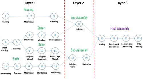
The manufacturing process of the stator is comprised of the following key manufacturing steps: sheet cutting, stacking, insulation, winding, and impregnation (Kißkalt et al., 2018). During sheet cutting and stacking, thin metal sheets are cut into specific sizes and shapes following tight tolerances using cutting techniques such as laser cutting or punching (Mayr, Lechler, et al., 2019). The resulting metal sheets are then stacked and joined with a welding technique or an adhesive to form the laminated core (Kißkalt et al., 2018). The laminated core is a critical component that holds the windings and the slot insulation and any deviation from the required tolerance can produce electrical faults in the coil (Sell Le Blanc et al., 2014). During winding, an enamelled copper wire is wound in a desired winding scheme to produce a magnetic field (Mayr et al., 2021). The final step is to impregnate the core to further improve the insulation and thermal conductivity of the stator.

The tendency of fault generation is high in processes involving deformable materials, especially when the deformable material, for example, the copper wire, is stretched beyond its yield limit (Mayr et al., 2021). This can cause a permanent deformation that affects the overall electrical resistance of the coil. Also due to its elastic properties, a springback effect is created affecting the position of the wire (Hagedorn et al., 2018). As a result, the coil winding process is highly prone to errors, and hence the quality of winding influences all the end-of-line tests, suggesting its very significant influence on achieving the required manufacturing standards (Tiwari et al., 2021). Due to these reasons, the coil winding process was selected as the main focus of this research.

2.1 Coil winding

An increasing demand on the quality of winding products, with tighter tolerances of electrical characteristics and geometrical dimensions, is a key challenge in the field of coil winding. For coil winding, different winding schemes are commonly used in the industry such as wild layer and orthocycling winding, with the last one in the list offering the highest fill factor (Hagedorn et al., 2018). Some of the commonly employed techniques used to perform an orthocycling scheme are linear, needle, flyer, and toroidal winding (Hagedorn et al., 2018). The linear winding technique, which is the focus of this research, is one of the most profitable techniques used in the industry for coil winding due to its simplicity and high reproducibility, where many coils can be wound at the same time using one machine (Sell Le Blanc et al., 2014).

2.1.1 Linear winding

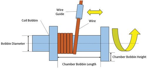
During linear winding, copper wire is pulled straight on the coil’s bobbin through a nozzle using a linear movement that is guided by a device called a wire guide, which moves horizontally throughout the length of the bobbin creating a winding scheme (Sell Le Blanc et al., 2014, 2015). A representation of a linear winding technique is presented in Figure 2. This set of movements ensures that the wire is laid following a predefined scheme and produces a higher fill factor at a high speed (Hagedorn et al., 2018). A correct laying of the wire where no geometrical faults occur will result in a higher fill factor of the bobbin (Sell Le Blanc et al., 2013). Another aspect that needs to be considered during linear winding is that the wire is introduced to several stresses during the process (Sell Le Blanc et al., 2015). As a result of applied stress or tension, the wire sometimes is pulled past its elastic limit causing deformation and a change in the cross-section of the wire (Hagedorn et al., 2018). As previously discussed (Hagedorn et al., 2018), this type of permanent deformation can influence the overall electrical resistance of the bobbin. This defect can only be detected once the bobbin has been completely wound by using an end-of-line test such as a DC high potential test (Mayr et al., 2021).

Figure 2. Ordinary linear winding process scheme (adapted from Hagedorn et al. (2018)).

2.1.2 Winding faults

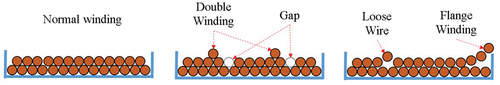
As discussed in previous sections, a majority of faults or defects in the stator are created during the winding process (Hagedorn et al., 2018). The main faults that occur during linear winding can be divided into two types: geometrical and electrical (Mayr et al., 2021). The first type of fault tends to appear when there is an improper laying of the wire on the surface of the bobbin leading to deviations in the winding schemes and a poor fill factor. This type of fault is caused by a variation in the speed of the wire guide, a lack of synchronisation between the rotational movement of the bobbin and wire guide, or a change in the wire’s diameter (Mayr et al., 2021; Sell Le Blanc et al., 2014). The most common geometrical faults found during linear winding are double winding, gap, loose wire, and flange winding (Sell Le Blanc et al., 2014), a representation of these faults is shown in Figure 3. The second type of fault is electrical, which occurs when the cross-sectional area of the wire is reduced due to the application of compressive and tensile stresses. A change in electrical resistance of the coil or winding with respect to increasing the fill factor of the coil has been investigated by Dobroschke (2011).

Figure 3. Common faults detected at a linear winding process with an orthocycling winding scheme.

2.2 Modelling techniques

Modelling techniques are increasingly being used across a range of industries to imitate real-world manufacturing systems and processes. Models allow an insight into how the process or system will perform under various situations. However, during manufacturing processes, correlations between input and output parameters are known to affect the creation of faults. Baier et al. (2019) point out that interdependencies can be detected to establish the level of influence that it has on the quality of the final product.

2.2.1 Modelling techniques for electric motors

Previous research has reported analysis of individual manufacturing steps using various modelling techniques, thus leaving a gap in our understanding of interdependencies between process parameters from various steps on the origin or occurrence of defects. Finite Element Analysis (FEA) has been used before to model and analyse the relationship between the physical properties and extreme vibrations in a stator system of a permanent magnet synchronous motor with concentrated windings (Chai et al., 2018). However, FEA may not be as efficient in identifying long-term interdependencies across an entire manufacturing process. de Oliveira et al. (2018) demonstrated the use of Convolutional Neural Networks (CNN) for quality tests in induction motors to inspect defects in the stator windings for induction motors. Karanayil et al. (2005) utilised Artificial Neural Networks (ANN) to create a model of an induction motor drive that accurately represents the variation in the electrical resistance of a rotor. Nevertheless, to develop an accurate and precise neural network, an extensive data set is required as input to start training the model, which is not easily available in complex manufacturing problems.

Currently, there is a range of techniques and tools that can be used to model the process and parameters in electric motor manufacturing, an example is the work by Ghandi and Masehian (2015) on modelling and online detection of stator faults in electrical motors. It is discussed that this area of research offers an opportunity to explore the behaviour of various manufacturing process parameters that fluctuate during the process and investigate the repercussions that they have on the final product quality (Ghandi & Masehian, 2015). Some modelling techniques in the context of EM manufacturing are discussed below:

Finite Element Analysis (FEA)

This technique has the capability to solve complex problems involving deformable bodies, heat transfer, and fluid (Zaeh & Siedl, 2007). FEA has been utilised to model stress and structural analysis of components such as the stator and rotor in an electric motor (Weigelt et al., 2019). However, this technique has some limitations: it is considered an expensive technique due to the high level of expertise and computational cost needed to run simulations and when dealing with complex problems this method tends to be time-consuming.

Neural Networks (NN)

NN is typically a supervised learning technique that uses algorithms such as backpropagation to identify relationships in sets of data during a manufacturing process that is both stochastic and predominantly non-continuous (de Oliveira et al., 2018). This technique has been used in quality inspections in electric motors in order to detect faults in the stator winding of induction motors (de Oliveira et al., 2018). Nevertheless, using NN in electric motors presents a challenge in cases where there is no extensive data set to start training the model. This is a possibility in complex manufacturing problems and, hence, NN will not be accurate enough and can become unreliable.

Petri Nets

A Petri net is a modelling technique that can describe and analyse the flow of information in a graphical form (Wang et al., 2014). This technique has been used in modelling and evaluating faults in electric vehicle manufacturing research to perform reliability analysis and decision-making (Wang et al., 2014). Gaied et al. (2017) obtained favourable results in monitoring and fault detection analysis by implementing a fuzzy diagnosis based on Petri Nets in a winding machine. The limitations of this technique are as follows: it is time-consuming, not statistically representative, and does not take into account the combined impact of multiple faults.

Discrete Event Simulation (DES)

Discrete Event Simulation (DES) has been utilised to support decision-making, focusing on production planning as a method for enhancing and evaluating system performance (Negahban & Smith, 2014). Albers et al. (2019) identified that there is potential in implementing the elements provided by Industry 4.0 such as simulation to model interdependencies between product and process parameters. They discussed that modelling relationships in a manufacturing process can result in a more controlled and stable process. Mayr, Lechler, et al. (2019) utilised DES modelling approach for analysing energy aspects in a production line. Paryanto (2017) demonstrated the use of DES as an approach for process planning and energy efficiency. Prajapat et al. (2020) explored the use of DES for decision-making in real-time while implementing the use of multi-objective optimisation methods such as random forests to improve objective functions in a turbine assembly process. Furthermore, random trees were introduced as an optimisation method to express the relationships that exist between input variables and conflicting objectives while also increasing the accuracy of the predictions.

Capocchi et al. (2008) utilised DES to model electric motor components such as the rotor and stator since it has been used before with promising results in a three-phase wound-rotor induction machine for early fault detection. By using DES in this case, the windings in the motor were protected and provided with efficient predictive maintenance (Budgaga et al., 2016). DES has previously been used for decision-making and visualising the relationship between input and output parameters in a turbine assembly process in the industry (Lomakin et al., 2020). DES has also been implemented in the reconfiguration of factory layouts, which tend to be time-consuming and expensive (Prajapat et al., 2019). In this case, a repair facility that required a reconfiguration for a new maintenance regime used a DES to model and assess various scenarios, which helped the decision-making process of a new layout planning. The innovation, in this case, was to merge the DES with immersive technologies such as Augmented Reality (AR) to provide the users with a new form of interaction with the simulations that have the potential for optimising shop floor activities. However, there have been no previous attempts to use the DES approach that takes into account process characteristics and interdependencies, thus providing a great opportunity for further research in this area.

Utilising a DES as a modelling technique offers greater advantages as compared to other techniques discussed above, for example, DES does not require an extensive database as in the case of Neural Networks to obtain accurate results when detecting relationships between parameters. The computational load in terms of memory and time is lower as compared to FEA. The fabrication of EM makes Petri nets limited and too simple when dealing with complex problems, while DES can be adapted to more complex problems easily. Finally, one of the main advantages that DES possesses is the fact that it considers the effect of multiple input and output parameters in a manufacturing process that helps to identify process interrelations.

2.3 Gap in literature and novelty of the work

As discussed in section 2.1.1, the typical geometry faults (such as crossover, gap, loose wire, and double winding), structural faults (such as bulging, convex or concave winding), and electrical faults (such as increased coil resistance) mainly result from the undesired variations in process parameters (Hagedorn et al., 2018). As a result, the coil winding process has a massive influence on the generation of geometrical and electrical faults. This emphasises on the requirement of a model that can simulate the variations in process parameters (such as wire tension, winding speed, and caster angle) and predict the state of the coil and the accumulated error. Currently, there is a lack of such simulation models capable of identifying and detecting the influence of process interdependencies in a complex manufacturing process for electric motors involving non-rigid deformable components. Nevertheless, to develop an accurate and precise neural network, an extensive data set is required as input to start training the model, which is not easily available in complex manufacturing problems. This data problem is solved using DES in this study/project.

This paper proposes a computational framework to model interdependencies in a complex electric motor manufacturing process, where the time dependency is a vital aspect while dealing with process parameters that affect the properties of deformable components during the manufacturing process. A DES model was created to simulate the variations in set process parameters (such as set wire tension with respect to winding speed, castor angle of the wire, shape and aspect ratio of the bobbin) and their impact on the final quality of the coil in terms of generated geometrical and electrical faults. The novelty of this simulation model is that it is capable of predicting faults and errors created at the end of each manufacturing step while considering the deformable properties of the copper wire. This leads to a reduction of quality tests such as the winding resistance test.

The accuracy and reliability of the DES model were validated with a series of experiments conducted using a linear coil-winding machine setup where key process parameters such as rotational speed, wire diameter, and shape of the bobbin were varied. The validation process also included presenting the model to experts from the EM manufacturing industry for their feedback and suggestions on the model. Furthermore, this simulation model can be implemented as an innovative tool to create a new robust database.

The remainder of this paper is organised into the following sections: an overview of an electric motor production process particularly focusing on coil winding and winding faults; the techniques used for modelling interdependencies in electric motors manufacturing; the methodology to develop the DES model for a linear winding process; the validation process by experiments on coil winding machine; results obtained from the simulation model and the lab-based coil-winding machine; discussion on validation by industry experts; directions for related future work and conclusions.

3. Methodology

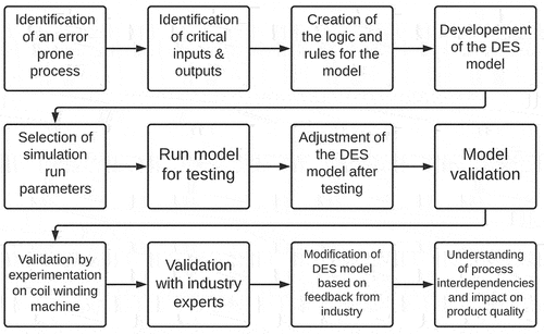
The research methodology used for the development of the simulation model is presented in Figure 4. The first step was to identify an error-prone process involving deformable material in an electric motor. The second step was to determine from literature the critical inputs and outputs in that manufacturing process. The third step was to create the logic and rules that the simulation model had to follow based on the relationship that input parameters have with output parameters (Hagedorn et al., 2018). The next step was to develop a DES model that follows the logic and rules previously set. The model was run using a design of experiments in which the key input parameters were varied to verify that the logic and the rules were followed appropriately. The model was verified and validated using two approaches: the first one was validation through experimentation and the second was through feedback from industry experts. This validation process was used to establish compliance of any process output as compared to inputs, providing evidence that the model performs as expected. Finally, the DES model was modified using the feedback provided by the industry experts.

Figure 4. Research methodology for the development of simulation model.

3.1 Identification of an error-prone manufacturing process

The first step was to conduct a thorough literature review to identify an error-prone process step during the manufacture of an electrical machine. A survey of industries involved in EM manufacturing (Tiwari et al., 2021) and a review of the literature (Sell Le Blanc et al., 2014) revealed that the stator is one of the components in an electric motor with the highest number of faults during manufacturing. During its fabrication, several manufacturing operations such as coil winding include deformable material, which tends to alter its shape at various stages of the process causing variation. This variation can have an influence on the generation of faults. As a result, coil winding was selected as an error-prone step during the stator’s manufacturing process.

3.1.1 Identification of first parameters

As Hagedorn et al. (2018) explains, certain process parameters such as winding speed have a stronger influence than others on the generation of faults. From the literature review, the key input parameters were identified, namely, winding speed, tension, wire diameter, and bobbin geometry, as shown in Table 1. Although these were the first parameters selected to be used in the DES model, more parameters were added to the model at a later stage. The table presents the input parameters, their range, and the output parameters from the model.

Table 1. Input and output parameters selected for the DES model.

Input parameters	Range	Output parameters
Winding speed	100–350 RPM	Electrical resistance value
Tension value	40–80 N	Electrical resistance accumulated error
Wire diameter	0.30–1.20 mm	Caster angle
Bobbin shape	1: Rectangular, 2: Square, 3: Circular	Geometrical faults

3.2 Development of a DES model for the linear winding process

The DES model was developed in Witness Horizon simulation software, by The Lanner Group Ltd (2021). The models were based on a literature review and the information obtained from industry experts. The software allowed modelling and simulation of a wide range of discrete events addressing complex industrial problems where time dependency is a vital aspect.

3.2.1 The logic and rules

The logic for the DES model was based on literature and represented the influence of process interdependencies on the winding process and generation of faults (geometrical or electrical) (Concettoni et al., 2012; Meyer et al., 2015). The DES model was designed to simulate the behaviour that input parameters have during the first five layers of the winding process. According to Hagedorn et al. (2018), the first five layers of the winding process present the highest number of faults due to the first contact of the wire against the bobbin’s surface. Once the first few layers of wire are set onto the bobbin surface, the next layers fit tightly into the grooves created by the copper wire (Hagedorn et al., 2018).

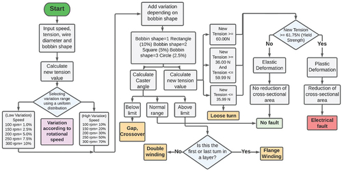
The winding scheme in the DES model was an orthocycling scheme, which is preferred in the industry due to its high fill factor (Hagedorn et al., 2018), comprised of five winding layers, and each layer had 20 turns. The DES model followed a logic depicted in the flowchart shown in Figure 5.

Figure 5. Flowchart of the logic used in the DES model that represents a linear winding process.

3.2.2 Features in the DES model

The DES model is composed of several process steps during the winding process. These steps include the storage of wire, the wire break, and the wire guide as shown in Figure 6. Storage is the first step in the winding process where the copper wire is slowly unwound from a larger bobbin and then fed to the winding machine. The DES model adds a small variation to the cross-sectional area of the wire to represent any abnormalities created during the wire’s fabrication. The wire break applies the first constant tension to the wire throughout the process. However, due to variations in the process parameters such as the winding speed, the applied tension by the wire break can vary impacting the cross-sectional area of the wire. The wire guide is the next step in the process, and its purpose is to allocate the wire to its final position over the bobbin’s surface. With a variation in winding speed, the wire can be misplaced and create a geometrical fault. Next is winding, during this step the wire has already been allocated to a determined position on the bobbin’s surface following a winding scheme. The winding scheme defines the order and position at which the wire is allocated throughout the bobbin to maintain a structure that reduces the space between turns (fill factor). The winding scheme also defines the number of turns and layers that need to be followed to complete a coil. During this step, the DES model follows an orthocycling scheme, which is the winding scheme with the highest fill factor.

Figure 6. Example of the DES model representing a linear winding process using the Software “Witness Horizon” (Lanner Group Ltd, 2021).

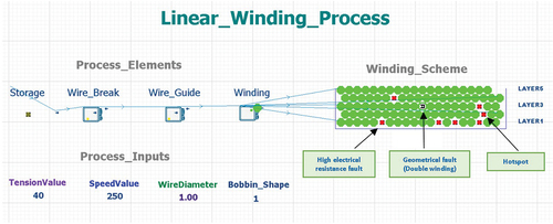
The model then calculates the accumulated electrical resistance variation of every turn as well as the caster angle that leads to the creation of geometrical faults. Further details about these process steps are explained in section 4. The output from the simulation model is (i) a winding scheme representation of every turn and layer during the winding process. This representation shown in Figure 6 (right side) presents the exact location of each turn as well as the turns that present a fault. These faults can be represented as a high electrical resistance fault, a geometrical fault, or a group of faults allocated together known as a hotspot. (ii) A database in the form of tables that include the electrical resistance value of every turn throughout the winding process. These tables also include the calculated caster angle of every turn and the type of geometrical fault created. This database will aid in the identification of the exact moment throughout the process where an abnormality is created, affecting any of the key process parameters such as the winding speed, tension, and cross-sectional area of the wire. The database will later be used as a training set for a supervised learning algorithm that will enhance the manufacturing process.

3.3 Validation by experiments on coil winding machine

The results from the DES model were validated by conducting experiments on a lab-based linear winding machine that was used to produce an orthocycling winding scheme. Figure 7a depicts the lab-based linear winding machine which is a model 200 mm CNC Coil Winder MK4. Figure 7b shows the Coil Winder Controller MKII Software V4.5 that allowed the user to control process parameters such as the speed, the bobbin size, and the number of turns per layer. The winding machine was capable of producing small quantity runs of coils or custom one-off coils for a vast range of bobbin shapes for electronic projects. The machine is fitted with closed-loop motors on both the feeder and bobbin assembly, which increases the torque, accuracy, speed, and number if losing steps. The highest winding speed capability of this machine was 2000 rpm.

Figure 7. Linear winding machine used for experimentation model ”200 mm CNC Coil Winder MK4”.

3.3.1 Experimental plan to validate simulation model

The first part of the validation process was performed through experimentation. A linear winding machine was used for testing by varying the key input parameters such as rotational winding speed, bobbin’s geometry, and wire diameter. A systematic approach was required to conduct the experiments in order to determine the effect that the key input parameters have on the process output product. A full factorial design of experiment’s approach has proven its effectiveness in terms of flexibility and low cost while reducing the cogging torque in an electric motor using variables such as dimensional tolerances (Islam et al., 2011) and to determine the best prototype option for the development and design of a new automated trickle winding process for an electric motor (Halwas et al., 2018). Therefore, a 2³ two-level full factorial design of experiments was used for experimentation.

These designs are known as screening designs and each design refers to k factors with two levels each. Each of the factors had two levels to identify potentially important input process parameters. The first factor was the rotational speed with two levels (low speed = 100 rpm and high speed = 800 rpm). The second factor was the bobbin shape with two levels (rectangular shape = 1 and square shape = 2). The last factor was the wire diameter with two levels (small gauge = 0.30 mm and large gauge = 0.71 mm). In this case, k = 3 and 2³ = 8 possible combinations. The eight different ways of combining the high and low settings are shown in Table 2.

Table 2. Standard order of the full factorial design of experiments for the linear winding process.

	Process Parameters
Run #	Rotational Speed (rpm)	Bobbin Shape	Wire Diameter (mm)
1	100	Rectangle = 1	0.30
2	800	Rectangle = 1	0.30
3	100	Rectangle = 1	0.71
4	800	Rectangle = 1	0.71
5	100	Square = 2	0.30
6	800	Square = 2	0.30
7	100	Square = 2	0.71
8	800	Square = 2	0.71

As previously discussed, input process parameters have a great influence on the creation of faults during winding. Therefore, two critical input parameters were selected for further analysis.

Bobbin shape

The shape of the bobbin has a huge influence on the creation of faults (Hagedorn et al., 2018). The shapes that create the most variation in the system are the square and rectangular bobbins, this is because the wire length between the wire guide and the winding location is continuously changing throughout the process (Hagedorn et al., 2018). This variation is minimal in the circular bobbin since the shape of the bobbin remains constant; therefore, circular bobbins were not considered for the experiments. The shape for each bobbin was designed using a CAD software (Fusion 360 (Autodesk, 2022)), and once the design for each bobbin was finalised, a 3D printed version of each one of the bobbins was created.

Wire diameter

The wire diameter has an important influence on the creation of faults. Dobroschke (2011) explains that a change in the wire gauge has a direct effect on the caster angle limit, the yield limit, and the spring back angle. The caster angle and yield limit tend to increase as the diameter of the wire increases; therefore, a thicker wire will withstand a larger tension resulting in less number of faults. Furthermore, the spring-back angle is created when a wire is laid on a surface and due to its elastic properties, it tends to return to its previous state with a spring-back effect. This springback angle is more noticeable in wires with a smaller cross-sectional area. Thus, having a large spring-back angle leads to wires moving from their intended position while winding producing geometrical faults. As a result, two different wire gauges (0.30 mm and 0.71 mm) were used for the experiments to analyse the influence that the diameter of a wire had on this process step. These two wire gauges are normally used in the industry and are in the range that appropriately fits the wire guide in the machine without causing any extra tension to the wire when it passes through the nozzle.

3.4 Validation with industry

The next part of the validation process was to demonstrate the simulation model to EM manufacturing experts from industry and academia, and simulation experts. Their feedback was recorded, and necessary amendments were made to the model.

4. Results from the DES model

The DES model required the following input parameters to be entered into the system: the rotational speed, tension, wire diameter, and type of bobbin shape (Figure 6). After receiving the input parameters, the model created variations in the set value of the applied tension based on the input values. The detailed working of the simulation model has been explained in section 3.2.2. Research suggests that in non-circular bobbins, higher winding speeds create a variation in the process parameters that affects the wire tensile force applied to the wire eventually leading to changes in the electrical properties of the wire. The DES model calculates the variation in applied tension where the tension value fluctuates (Sell Le Blanc et al., 2015). Application of tension beyond the yield limit can cause a deformation in the wire and reduce the cross-sectional area of the wire, leading to increased electrical resistance in that region. To calculate the electrical resistance of a wire, firstly, the electrical resistance of copper was calculated using Eq. 1:

(1) $R_{Cu}=\frac{{\rho }_{Cu}}{A_{Cu}}=\frac{4\cdot {\rho }_{Cu}}{\pi \cdot d_{Cu}}$(1)

where the resistivity is represented by ρ (1.72 × 10⁻⁸ Ωm) and then divided by the cross-sectional area of the copper wire ($A_{Cu})$. Moreover, in literature, it is described that the fill factor affects the electrical resistance of a coil (Dobroschke, 2011). When the fill factor of a coil is reduced, the electrical resistance in the wire increases. This is caused because the smaller the fill factor in a coil, the more spaced between the wires leading to greater electrical resistance. In addition, the geometries of the coil determine the degree of influence that the fill factor has on the electrical resistance when maintaining the same number of turns in the coil. Thus, having a bigger winding space, the influence of the fill factor over the coil’s electrical resistance tends to be smaller. However, research has shown that researchers tend to focus their efforts on calculating the electrical resistance value of a coil only after being wound (Dobroschke, 2011). However, during the winding process certain process parameters affect the diameter and the cross-sectional area of the wire leading to electrical faults. Wolf (1997) explains that the most important parameter that has the greatest influence on the electrical resistance is the diameter. He explains that there is a clear interdependence between the decrease in the diameter and the increase in electrical resistance and it can be analysed by using the next equation:

(2) $\mathrm{\Delta }R=R1-R0=\frac{4L_1\cdot \rho }{\pi \cdot {d_{nom1}}^2}-\frac{4L_0\cdot \rho }{\pi \cdot {d_{nom0}}^2}$(2)

A reduction in the diameter ($d_{nom1})$ leads to a reduction in the current carrying area, thus an increase in the electrical resistance. As it was pointed out, in multi-layering, a smaller diameter of the wire leads to a reduced length considering the same number of turns since the wires are now laid tighter (Wolf, 1997). This creates a smaller cross-sectional area leading to an increase in electrical resistance. Therefore, fluctuations in the process or the product tolerances often lead to inconsiderable variations in the electrical resistance (Wolf, 1997).

Komodromos et al. (2017) demonstrated in an experiment the effect that the tensile force has on different copper wire diameters and the effects it creates on the electrical resistance. These copper wires were strained until their cross-sectional area changed and then measured the change in electrical resistance showing that wires with a smaller diameter (0.63 mm) had an increase in electrical resistance of 23%, while wires with a larger diameter (1.18 mm) only had an increase of 8% in their electrical resistance. Dobroschke and Wolf agree that the main problem is that the electrical resistance of a wire cannot be determined directly during the winding process since it will damage the insulation.

Therefore, a model that can accurately model process interdependencies that lead to faults during winding was developed. This model was able to calculate the variation of the wire diameter, cross-sectional area, and length during each turn. Having the electrical resistance of each turn will allow the user to determine any hotspots in the coil during winding, resulting in a time reduction for quality tests. Furthermore, an important feature in the DES model was the identification of the exact location of faults during winding that highlighted a region if the faults lay in close vicinity of each other, i.e., a hotspot.

A representation of the orthocycling scheme was designed to represent the winding scheme in the model as shown in Figure 6, in which each turn was represented by a circle where the colour or text in the circle represented fault or no-fault in that turn depending on the process parameter values. For example, during winding when the set tension was under the established yield limit, no reduction of the cross-sectional area was reported and the turn is displayed as a green circle representing a non-faulty turn. In cases where the variation in the value for the set tension exceeds the yield limit of the copper wire, an electrical fault (area of increased electrical resistance) is displayed as a red circle instead of a regular green circle. Moreover, when a few turns with geometrical or electrical faults lie in the vicinity of one another, they are represented as a region of a local hotspot.

A feature was added to the simulation model to calculate the cumulative increase in electrical faults in the winding system. This feature determined the stage at which the increase in electrical resistance exceeds beyond a set threshold making the winding unsuitable for use. To obtain the cumulative error, the percentage error in every turn of each layer was calculated and added as the winding progressed. After the discussion with the industry experts, the threshold value for cumulative error in electrical resistance was set as 10% for this model and the model was set to stop the process when this value is reached to avoid producing nonviable coils.

Based on the values of process parameters and any variations, a set of rules (presented in Table 3) established the generation of a specific type of geometrical fault (Hagedorn et al., 2018; Meyer et al., 2015). As shown in Table 3, some types of faults in lower layers can lead to further generation of faults in the top or adjacent layers, hence affecting the overall winding scheme. Therefore, it was important to consider the faults (electrical and geometrical) in previous turns or layers before determining the electrical and geometrical in the next turns or layers.

Table 3. Rules for the selection of geometrical faults adapted from (Hagedorn et al., 2018), (Meyer et al., 2015).

Faults	Symbol	Rules	Produces
Flange Winding	F	Only appears at the beginning of each layer when the tension is above the yield limit	Gap, Cross over and Double Winding
Gap	G	It is produce anywhere in the coil under low or high tension	N/A
Cross Over	C	Occurs only during high tension and it can be located in any turn or layer	Double winding
Double Winding	D	Only is created after the second layer and when the tension is over the yield limit	Multiple Winding, Gap
Multiple Winding	M	It can be produce after a double winding and sometimes by it self after the yield limit is reach	N/A
Bulgy Turn	B	This fault appear when the tension is under the 35 newtons in any layer or turn	Bulgy Turn
Loose Wire	L	It only appears at the end of the winding process if there is a low tension	Problems during contacting

In order to represent a geometrical fault in the simulation model, the caster angle value was calculated for each of the turns based on the position of the wire guide and the wire on the bobbin’s surface (Hagedorn et al., 2018). When the model detected that the caster angle value was out of range, it was categorised as a geometrical fault. The geometrical faults were represented by the initial letter for each fault as shown in Table 3 and displayed inside of each turn (Figure 6). The DES model used this approach to represent when a geometrical fault appeared in the winding and define the type of fault. Results showed that the most common fault that occurred during winding was a double winding, whereas the geometrical fault that appears the least was flange winding. This is the least common fault because flange winding can only appear on the edges of the bobbin, limiting the number of faults. Unlike, the rest of the geometrical faults that can occur at any point during winding.

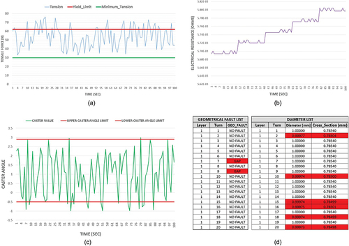
The DES model provided the value of the parameters applied to the wire for every layer and turn in a rectangular bobbin at a high speed as shown in Figure 8. Figure 8(a) shows the variation that the tension value had throughout the winding process and presents an upper boundary (yield limit) that, when exceeded, leads to an electrical fault. The graph also presents a lower boundary that once reached a loose winding occurs due to the lack of tension in the wire. Figure 8(b) demonstrates the variation in electrical resistance during winding and presents the incremental step after each layer in the bobbin. Figure 8(c) shows the variation in the caster angle, faults, and the effect that a reduction of the diameter in the copper wire has on the cross-sectional area. Since the copper wire is a deformable material, it is important to identify the location where there has been a change, and when the upper and lower limits were reached, different geometrical faults such as a gap were created. Figure 8(d) presents two example lists obtained from the DES model that highlight the location of geometrical faults and the effect that a reduction of the diameter in the copper wire has on the cross-sectional area. Since the copper wire is a deformable material, it is important to identify the location where there has been a change in the cross-sectional area as this may impact the quality of the winding scheme with the generation of an electrical or a geometrical fault.

Figure 8. Tension chart of the DES model using a rectangular bobbin.

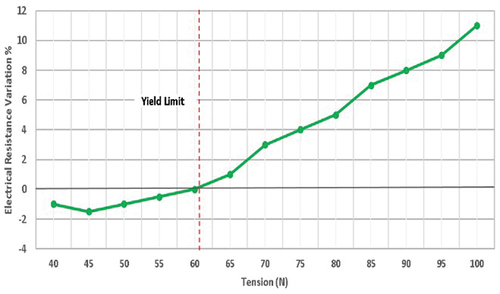
The results from the DES model also showed that variation in critical input parameters has an impact on the origin of faults such as increased electrical resistance. The model highlighted two main relationships between critical process parameters: the first between wire tension and electrical resistance and the second between the wire gauge, wire guide, and caster angle. The graph in Figure 9 demonstrates an influence on the increase in variation of the electrical resistance in a rectangular bobbin with respect to tension in the wire. This variation in the electrical resistance reached a level of 11% when the tension value (represented by a solid green line) went beyond the yield limit (represented by a red dashed line) by almost 40 N. The graph shows the point of transition between the elastic and plastic deformations marked by the established yield limit (61.75 N) for an annealed copper wire with a diameter of 0.71 mm. The yield limit marks the point at which the copper wire returns to its original diameter due to elastic deformation. Meanwhile, beyond the yield limit (plastic deformation area) the increasing tension produces a smaller diameter for the wire leading to an increase in electrical resistance. This causes a problem in the overall electrical resistance of the coil affecting the performance and reliability of the motor.

Figure 9. Plot showing variation in electrical resistance for a rectangular bobbin with respect to tension in the wire, the red dashed line shows the yield point of the wire.

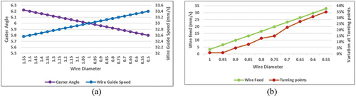
In addition, the DES model showed that parameters such as the wire’s diameter affected the wire guide speed and caster angle as shown in Figure 10 (a). Graph (a) displays a variation in the wire’s diameter when the wire guide speed (blue line) increases, leading the caster angle (purple line) to decrease from 6.2 to 5.8 degrees.

Figure 10. (a) Variation in winding speed and caster angle with respect to the diameter of the wire. (b) Relationship between wire diameter, wire feed rate and variation of wire guide at turning points.

The DES model calculated the caster angle using the following equation (Dobroschke, 2011):

(3) $CA=A+B\cdot ln\left(d_b\right)$(3)

The caster angle is calculated by multiplying the natural logarithm ($ln$) of the bobbin’s diameter ($d_b$) times the sum of the A and B angles created between the wire guide and the winding location. A angle is created between the winding location and the point exactly in front of the wire guide. The B angle is located in front of the wire guide between the tip of the wire guide and the winding location. Once the caster angle was calculated, the DES model calculated the maximum caster angle limits with the next equation (Dobroschke, 2011):

(4) $C{A}_{max}=-+0.4\cdot \left[A+B\cdot ln\left(d_b\right)\right]$(4)

The maximum caster angle was considered as the upper and lower boundaries in which no geometrical faults occur. However, when too much variation appeared in the process due to an increase in rotational speed and the caster angles were beyond the safety limits, a geometrical fault was created. These results showed that variation in the wire’s diameter causes the wire to become lighter and this new weight has an influence on the wire guide velocity, which was calculated using equations 4.1 and 4.2. To calculate the new wire guide velocity, the wire guide’s acceleration must be calculated using the equation 4.1.

(5) $a=\frac{F}{m}$(5)

The equation shows that the force applied to the wire guide is divided by the new combined mass of the copper wire and wire guide. Then with acceleration, the new wire guide’s velocity can be calculated using equation 9.2, in which the initial speed is added to the acceleration multiplied by the elapsed time.

(6) $v=v_0+at$(6)

Normally, during winding the initial position of the wire guide is located behind the winding location (where the wire touches the coil) to create a positive caster angle that allows the wire to be tense and produce a good winding scheme. However, results showed that when the wire guide speed increases due to a lighter wire, the caster angle decreases because in every turn the wire guide gets closer to the winding location. When the wire guide surpasses the winding location and the caster angle becomes negative, geometrical faults such as gaps tend to appear. The opposite effect occurs when the wire guide becomes too slow due to a heavier wire. The wire guide starts to pull the wire in the opposite direction to the winding placing it on top of the previous turn creating a double winding fault. The result of this interdependency between the wire’s diameter, the wire guide speed, and the caster angle creates a bulgy, convex, or concave winding geometry that leads to a low fill factor for the coil.

Figure 10b shows that a reduction in the wire’s diameter to half its size increases both the wire’s feed represented as the green line to almost 40% more speed and the amount of variation (red line) when stopping at the turning points by over 35%. As previously discussed, having a lighter wire causes the wire guide to increase its speed but also increases the speed of the actual wire. When the speed of the wire increases (wire feed), it has an influence the amount of variation at the turning points. The turning points are the points during winding where the wire guide must stop to change its direction to start a new layer. The DES model calculated the variation when stopping at the turning points by calculating the distance travelled by the wire guide after starting to deaccelerate using the following formula:

(7) $s=vt+\frac{1}{2}a{t}^2$(7)

Eq. 5 calculates the displacement from the wire guide from the point where it starts to stop to reach the turning point. The displacement (s) is calculated when the velocity of the wire guide ($v$) is multiplied by the elapsed time ($t$) and then add half of the acceleration ($a$) times the elapsed time square ($t^2$). The variation is created because the wire feed increases and creates a momentum that does not allow the wire guide to stop at the exact turning point, causing the wire in the next layer to be misallocated. This is an accumulative error that with every turn more wires are not placed in the right position creating geometrical faults and possibly a low fill factor. As a consequence, the variation is then calculated by obtaining the percentage difference between the turning point and the actual point where the wire guide stops which could be before or after the turning point depending on the acceleration of the wire guide.

Hence, using a DES model has proven the ability to identify and model correlations between parameters in an error-prone process that involves deformable material. This approach could be utilised to further analyse next manufacturing steps such as joining.

5. Validation experiments on coil winding machine

5.1 Electrical resistance faults

The experiment with the linear winding machine demonstrated the effects of changing process parameters such as the winding speed, wire diameter, and bobbin shape on the occurrence of faults. The first parameter to be measured was the electrical resistance variation of the wire, which was measured using a FLUKE 8808A bench digital multimeter. The resistance of the wire length used for experiments was measured before and after each experiment to record any changes in values. The rotational speed was varied for each experiment according to the full design of the experiments. The recorded values have been plotted in Figure 11 which shows the relationship between the winding speed and the variation in the electrical resistance while comparing different bobbin shapes.

Figure 11. Electrical resistance variation percentage with different wire gauges and bobbin shapes.

Winding speed and change in electrical resistance

The results from the experiments in Figure 11 show that the highest increase in electrical resistance was observed for cases when a rectangular bobbin was used and when the winding speed reached 800 rpm. The trend showed that when the rotational speed of the winding machine was increased, the variation in electrical resistance increased as well. In particular, it was noticed that the smallest change in electrical resistance variation was always presented at low speeds. This shows that there is a clear relationship between the winding speed and the increase in electrical resistance during winding.

Bobbin shape and change in electrical resistance

The relationship between the bobbin shape and the change in electrical resistance was also analysed. The rectangular bobbin presented on average an increase in electrical resistance of 4% at high speeds, while in comparison, the square bobbin only presented an average increase of 2.7%. The shape of a bobbin mostly depends on the aspect ratio, which defines the height and base of a bobbin. The results showed that having a larger aspect ratio of 1:6 (rectangle) causes the bobbin to have almost double the amount of variation in electrical resistance. However, in comparison, when using a square bobbin with an aspect ratio of 1:1, the variation in electrical resistance tends to be lower. This shows that a rectangular shape in a bobbin has a more significant impact on the electrical resistance.

Wire gauge and change in electrical resistance

The results also gave insight into the relationship between the wire gauge and the change in electrical resistance. Results showed that a larger wire diameter leads to a larger increase in electrical resistance. However, the increase in electrical resistance between the large and small wire gauge while using a square bobbin was far greater, reaching almost a 2% increment in electrical resistance. While the difference in variation between the large and small wires when using a rectangular bobbin was only 0.2%. This shows that different wire gauges have a different impact on the electrical resistance depending on the shape of the bobbin.

5.2 Geometrical faults

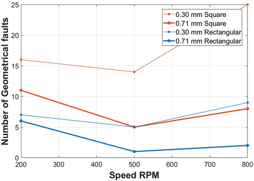
During experimentation, videos of the winding scheme were recorded to monitor and study the creation of geometrical faults. The videos of each run were analysed frame by frame using a checklist to mark the type and location of geometrical faults in the winding scheme. An example of a video frame representing a trial run with a square bobbin displaying geometrical faults such as gaps, crossings, and double windings while running at high speeds (800 rpm) is shown in Figure 12. From the images obtained, the number of geometrical faults that occur at different winding speeds was also recorded and presented in the form of a plot as shown in Figure 13.

Figure 12. Geometrical faults during linear winding at 800 rpm using a square bobbin.

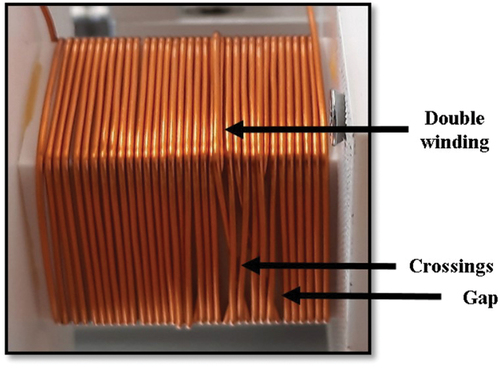
Figure 13. Plot with the number of geometrical faults at different winding speeds variating input parameters.

Winding speed and geometrical faults

The plot in Figure 13 shows that the highest number of geometrical faults tends to appear at low and high winding speeds, for example at 200 and 800 rpm. Results also showed that at a mid-range speed (500 rpm), the number of faults tends to decrease for both bobbin shapes. However, after this point, when the speed increases the number of faults increases as well leading to a similar number of faults as the ones obtained at low speeds. Therefore, a trend is created that causes the number of faults to increase and decrease as the winding speed increases. This shows that there is a correlation between the winding speed and the number of geometrical faults during winding.

Bobbin shape and geometrical faults

Figure 13 demonstrates that the shape of the bobbin affects the number of geometrical faults that appear in a winding scheme. It was discovered that a square bobbin has on average a far greater number of geometrical faults than a rectangular bobbin. It can be noticed that at low speeds the square bobbin had more than double the number of faults than with a rectangular bobbin. At mid-range speed both bobbin shapes had a similar number of faults except with the smaller gauge wire for a square bobbin in which the number exponentially increased to almost three times the number of faults produced with the other bobbins. Then, at high speeds, the rectangular bobbin tends to have the lowest number of faults with only two faults while in comparison, the square bobbin had eight faults at high speeds.

Wire gauge and geometrical faults

Figure 13 results show that the wire gauge also has an important effect on the creation of geometrical faults. This effect can be seen when using a smaller wire gauge. In both cases (square and rectangle shapes), the smaller wire gauges created more faults than a larger wire gauge. Using a thicker wire creates fewer geometrical faults in the winding scheme for both types of bobbin shapes; for example, in the case of the square bobbin, the thinner wire created 25 faults while with the thicker wire only 9 faults were created at high speeds. This shows that a smaller wire gauge has a greater impact on the creation of geometrical faults.

6. Discussion

The purpose of this research was to model interdependencies in a complex electric motor manufacturing process that involves deformable material. This was conducted by creating a DES model that simulates the variations in set process parameters and their impact on the final quality of the wound coil in terms of generated geometrical and electrical faults. A review of literature highlighted that the deformable properties of copper wire were not taken into consideration during the modelling of process parameter interdependencies and their influence on the creation of faults (Dobroschke, 2011). The results from the simulation model showed that input parameters such as winding speed and tension were critical factors in the creation of defects during coil winding (Escudero-Ornelas et al., 2021).

The simulation model demonstrated that when the winding speed was increased, it created a variation in tension between the wire guide and the winding location at the bobbin. This action created a variation in tension that affects the electrical properties of the copper wire. The yield limit marks the boundaries between elastic and plastic deformation impacting the diameter of the wire temporarily or permanently. When this limit was surpassed, it caused a permanent reduction of the cross-sectional area in the wire, thus increasing its electrical resistance. The increase in electrical resistance leads to further faults down the production line such as short circuits and reduces the overall performance of the electric motor.

6.1. Electrical faults: comparison of results from simulation model and physical experiments

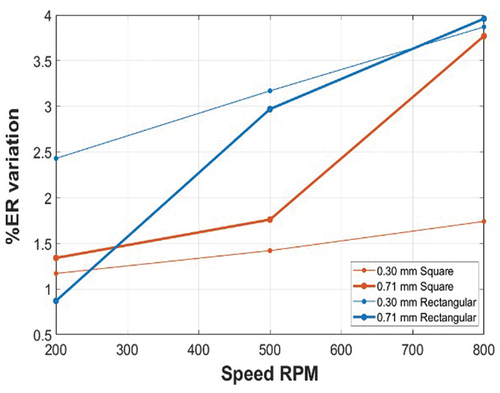
The results from the DES model were validated by conducting a series of experiments in a lab setting using a linear coil-winding machine where key process parameters varied. The results from the DES model and the experiments were also compared to understand the accuracy of the model. To evaluate the performance of the DES model against the experiments, the electrical resistance variation on the wire was analysed as shown in Figures 14 and 15. Figure 14 presents the correlation between the rotational speed and the electrical resistance percentage variation using a rectangular bobbin, while Figure 15 uses a square bobbin. In the figures, a series of experiments were represented as straight lines, while the DES model is presented as dashed lines. Each figure presents two scenarios where different wire thicknesses were employed: the blue lines represented a thicker wire (0.71 mm) and the red lines represented a thinner wire (0.30 mm). Figures 14 and 15 show that there is a correlation between the winding speed and the percentage variation in the electrical resistance of the bobbin. It can be noticed that in both cases (rectangular and square bobbins), a higher percentage variation is presented with thicker wires. This effect is more noticeable at higher speeds where the percentage variation increases up to 4% as seen in Figure 14. However, in both figures, the DES model and the experiments shared the same trend to increase its variation when the winding speed increases. However, the rectangular bobbin shows overall a larger variation compared to the square bobbin in which only at higher speeds and with thicker wires the variation starts to increase from 1.3% to 3.7%.

Figure 14. Comparison for a rectangular bobbin with two different wire gauges using a DES model and linear winding experiments to determine the percentage error in electrical resistance.

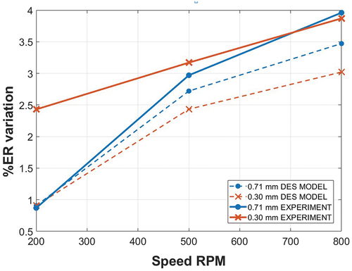
Figure 15. Comparison for a square bobbin with two different wire gauges using a DES model and linear winding experiments to determine the percentage error in electrical resistance.

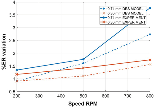
The results confirmed that the shape of the bobbin plays a key role in the increase in the percentage variation of the electrical resistance in the copper wire. It can be noticed that the rectangular bobbin tends to create a higher variation even from slow winding speed. Whereas, with the squared bobbin, the variation percentage remains low until higher speeds were reached. This is due to the aspect ratio of the bobbin shape and the influence that it has on the tension. Having a greater aspect ratio causes the tension to fluctuate rapidly throughout the process and surpass the yield limit. Meanwhile, with the square bobbin, the aspect ratio remains constant during the process, thus leading to less variation during winding. This is critical for manufacturers since taking into consideration the shape of the bobbin can reduce the variation in electrical resistance and improve the quality of the coil.

Furthermore, experimenting with different wire gauges during this research presented a correlation between the winding speeds and wire diameter. The comparisons between the DES model and the experiments showed that the wire with a larger diameter tends to deform more easily at higher speeds producing higher electrical resistance. Similarly, one of the key aspects to notice from the DES model in comparison to the experiments was that with a smaller wire diameter the least amount of electrical resistance variation was presented. One of the reasons for this behaviour can be that in the DES model no other input parameters apart from the selected ones were considered. For example, friction in the wire guide could be an input parameter that affects the creation of faults during winding by applying extra tension to the wire. However, currently the DES model does not consider all of the possible input parameters that influence the creation of faults, it only considers the three that have the highest influence (Sell Le Blanc et al., 2014). However, for future research, more input parameters can be added to the simulation model to improve its accuracy.

Subsequently, the percentage error or difference between the results from the DES model and the physical experiments (Figures 14 and 15) was also analysed to determine the accuracy of the model. The percentage error is the difference in the trend between the DES model and the experiments using the linear winding machine. Table 4 presents the percentage of difference in electrical resistance between the DES model and the experiments. For the case of the rectangular bobbin, the thinner wire (0.30 mm) presented the highest percentage of error between the model and the experiment having a percentage of 1.56%. This can be attributed to external factors such as the environment, the material handling, and the machine tear and wear. Whereas, in the case of the square bobbin, the error was smaller with 0.27%. Overall, it can be defined that the square bobbin possesses a lower percentage error making this model the most accurate out of the two. Nevertheless, it has to be noted that the percentage error for both cases stayed under 5% making them accurate and reliable models.

Table 4. The Percentage Error results for the rectangular and square bobbins when calculating the electrical resistance.

	Rectangular bobbin
	200 RPM	500 RPM	800 RPM
0.71 mm	0.02%	0.25%	0.49%
0.30 mm	1.56%	0.74%	0.85%

The cumulative error was also calculated for the different scenarios used with the DES model as shown in Table 5. The cumulative error of the DES model is the percentage difference between a regular electrical resistance and a high electrical resistance during winding. This error was recorded and added for every turn until the simulation process was finished. Table 5 shows that the cumulative error tends to increase as the winding speed increases for both types of bobbin shapes. However, the rectangular bobbin presented a higher cumulative error than the square bobbin. This was due to the constant change in the wire length during winding which was more noticeable with rectangular bobbins than with square bobbins due to its shape. The change in the wire length has been shown to possess a greater effect on tension and electrical resistance, leading to a higher cumulative error. The variation in the wire diameter also showed that thicker the wires produced a higher error. Normally, thicker wires when stretched tend to be more brittle and lead to higher electrical resistance.

Table 5. The cumulative error results for the rectangular and square bobbins when calculating the electrical resistance in the DES model.

a
	Rectangular bobbin
	200 RPM		500 RPM		800RPM
0.71 mm	0.90%		2.60%		3.47%
0.30 mm	0.89%		2.45%		3.01%
b
		Square bobbin
		200 RPM		500 RPM		800 RPM
0.71 mm		0.43%		0.16%		1.04%
0.30 mm		0.27%		0.31%		0.19%

6.2. Geometrical faults: Comparison of results from simulation model and physical experiments

To evaluate the performance of the DES model regarding the detection of geometrical faults on the first layer of the bobbin, two plots were developed as shown in Figures 16 and 17. From the figures, it was observed that the DES model and the experiments presented a higher number of geometrical faults at high speeds. Similarly, both the DES model and the experiments presented a high number of faults at low speeds. The reason behind this was that the wire guide normally is ramping up and down affecting the caster angle and thus the laying of the wire creates more geometrical faults at these points. It was also determined that this phenomenon normally affects to a higher degree the thinner wires since they have a larger springback effect than thicker wires.

Figure 16. Comparison for a rectangular bobbin with two different wire gauges using a DES model and linear winding experiments to determine the number of geometrical faults in the first layer.

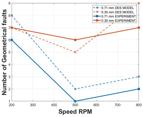
Figure 17. Comparison for a square bobbin with two different wire gauges using a DES model and linear winding experiments to determine the number of geometrical faults in the first layer.

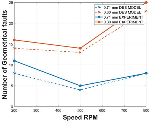
Furthermore, at mid-range speed, the number of geometrical faults tends to decrease, as the caster angle is more stable at this speed. The main difference between both plots (Figures 16 and 17) was that with the square bobbin the number of faults was considerably greater. In some cases, the number of faults increased to more than double. For example, when using a thinner wire with a rectangular bobbin at low speed, the number of faults was only seven. Meanwhile, using the same configuration but a different bobbin shape (square), the number of faults increases to 16. This showed that having a smaller aspect ratio (1:1) in the case of the square bobbin generated more geometrical faults in a coil during winding.

Also, from the plots shown in Figures 16 and 17, it can be determined that the winding speed has a great impact on the creation of geometrical faults. This is because during high speeds, the wire guide moves fast and misses its turning points leading to changes in the caster angle eventually causing the wire guide to be desynchronised with the bobbin leading to poor placement of the wire. This effect also causes the caster angle to gradually start increasing until it creates a geometrical fault such as a gap or a double winding. Having a positive caster angle under the established limits depends partially on the aspect ratio of each bobbin and the variation in speed. Thus, having both parameters under control leads to a correct winding scheme. To address this, control features can be implemented that can keep the caster angle constant throughout the process. The solution would be to calculate the specific turning points that adapt to the current winding speed, that way even at high speed the wire guide would be able to stop at the right point and keep the caster angle stable.

Additionally, the comparison between the DES model and the experiments showed that thinner wires tend to create more geometrical faults than thicker wires. This happens due to their spring-back effect as previously discussed in section 3.3.1, in which thinner wires have a higher tendency to spring back after being laid on the bobbin. It is recommended that to avoid this problem, the diameter of the wire remains constant during the process.

The DES model was also validated by obtaining feedback from experts in the field of simulation and electrical motor manufacturing. The experts agreed that the DES model was capable of identifying process relationships and their impact on the final quality of the winding. They responded that currently there was no model available that detected faults during winding and provided their exact location in the bobbin. This model could be useful to manufacturers since the electrical resistance for each turn can be known, adding confidence to the end-of-line tests. The limitation of the validation process is that the experiments only consider two different wire gauges to represent the lower and upper bounds of the spectra. However, further experiments can be carried out to analyse the effect that variation in a wire diameter on the electrical resistance of a bobbin after coil winding. Finally, the experts suggested that this model can be tested against further winding techniques, for example, needle winding.

7. Conclusions and future work

Electrical motor manufacturing process comprises complex manufacturing steps that involve deformable material. Due to the interdependencies in the process parameters in this complex process and the deformability of the coil, defects are accumulated creating a downstream effect on the process and the end product. This can be avoided by detecting faults early in the process. This can be achieved if critical process parameters and their interrelation with the creation of faults are identified. This paper proposed a DES model that models interdependencies in a complex environment for the production of electric motors, where time dependency is a key element while dealing with process steps that affect the deformable properties of copper wire. The DES model simulates the behaviour of the copper wire in each turn during the coil-winding step. The model was able to identify the applied wire tension, winding speed, the shape of the bobbin, and the diameter of the wire as key input parameters. The model captured electrical and geometrical faults in the wound coil as soon as they appeared and was able to calculate accumulated faults in the final wound coil highlighting any hotspot regions.

To validate the model, a linear winding machine was used to perform experiments where critical parameters were varied to analyse the influence that it has on the creation of faults. The model was also presented to experts to get their views and feedback as part of the validation process. The results from the experiments and the feedback from the experts determine that the DES model was able to identify how input parameters such as the winding speed and wire tension influence the creation of geometrical and electrical faults.

The future work for this research would be to combine the developed simulation model with the tools that Industry 4.0 has to offer, such as machine learning and digital twin. There is an expanding development in adapting these approaches to achieve an autonomous system (Khan et al., 2020). By implementing both concepts it is possible to have an integrated, robust, fast response and flexible manufacturing environment (Onaji et al., 2022). This system would be capable of predicting process faults by feeding in real-time data into a DES model.

Then, the data obtained from the DES model can be used as a database (and constantly be updated with new data) to be fed into an artificial neural network that can be trained to predict the current state of a component. This approach will allow the neural network to learn how interdependencies influence the creation of faults in the various steps that a complex manufacturing process has and minimise the effects as much as possible by selecting the optimal setting for each step in real-time.

This will drastically reduce the time and cost required for quality inspections after each step by directing the attention to only faulty areas (hotspots).

Acknowledgments

The authors would like to thank Airbus and the Royal Academy of Engineering under the Research Chairs and Senior Research Fellowships scheme. The co-author IOEO would like to thank the Mexican National Council of Science and Technology (CONACYT) for supporting his Ph.D. programme. For the purpose of open access, the author has applied for a Creative Commons Attribution (CC BY) licence to any Author Accepted Manuscript version arising.

Disclosure statement

No potential conflict of interest was reported by the authors.

Additional information

Funding

This project was supported by the Engineering and Physical Sciences Research Council of the UK through the Future Electrical Machines Manufacturing Hub (EP/S018034/1).

References

- Albers, A., Stürmlinger, T., Mandel, C., Wang, J., de Frutos, M. B., & Behrendt, M. (2019). Identification of potentials in the context of design for industry 4.0 and modelling of interdependencies between product and production processes. Procedia CIRP, 84, 100–105. https://doi.org/10.1016/j.procir.2019.04.298
- Autodesk. (2022). Fusion 360 | 3D CAD, CAM, CAE & PCB cloud-based software (Version V.2.014569) [Computer software]. https://www.autodesk.co.uk/products/fusion-360/.
- Baier, L., Frommherz, J., Nöth, E., Donhauser, T., Schuderer, P., & Franke, J. (2019). Identifying failure root causes by visualizing parameter interdependencies with spectrograms. Journal of Manufacturing Systems, 53, 11–17. https://doi.org/10.1016/j.jmsy.2019.08.002
- Budgaga, W., Malensek, M., Pallickara, S., Harvey, N., Breidt, F. J., & Pallickara, S. (2016). Predictive analytics using statistical, learning, and ensemble methods to support real-time exploration of discrete event simulations. Future Generation Computer Systems, 56, 360–374. https://doi.org/10.1016/j.future.2015.06.013
- Capocchi, L., Federici, D., Yazidi, A., Henao, H., & Capolino, G. A. (2008). Asymmetrical behavior of a double-fed induction generator: Modeling, discrete event simulation and validation. In MELECON 2008-The 14th IEEE Mediterranean Electrotechnical Conference (pp. 465–471). https://doi.org/10.1109/MELCON.2008.4618479.
- Chai, F., Li, Y., Pei, Y., & Li, Z. (2018). Accurate modelling and modal analysis of stator system in permanent magnet synchronous motor with concentrated winding for vibration prediction. IET Electric Power Applications, 12(8), 1225–1232. https://doi.org/10.1049/iet-epa.2017.0813
- Concettoni, E., Cristalli, C., & Serafini, S. (2012). Mechanical and electrical quality control tests for small DC motors in production line. IECON 2012 - 38th Annual Conference on IEEE Industrial Electronics Society, pp. 1883–1887. https://doi.org/10.1109/IECON.2012.6388914.
- de Oliveira, B. C. F., Seibert, A. A., Fröhlich, H. B., da Costa, L. R. C., Lopes, L. B., Iervolino, L. A., Demay, M. B., & Flesch, R. C. C. (2018). Defect inspection in stator windings of induction motors based on convolutional neural networks. In 2018 13th IEEE international conference on industry applications (INDUSCON) (pp. 1143–1149). https://doi.org/10.1109/INDUSCON.2018.8627172.
- Dobroschke, A. (2011). Fertigungstechnik - Erlangen: Flexible Automatisierungslösungen für die Fertigung wickeltechnischer Produkte. Meisenbach Verlag Bamberg. https://doi.org/10.25593/978-3-87525-317-7
- Escudero-Ornelas, I. O., Tiwari, D., Farnsworth, M., & Tiwari, A. (2021). Modelling interdependencies in an electrical motor manufacturing process involving deformable material. In Advances in Manufacturing Technology XXXIV: Proceedings of the 18th International Conference on Manufacturing Research, Incorporating the 35th National Conference on Manufacturing Research, 7-10 September 2021, Derby, UK (15, 291). IOS Press. https://doi.org/10.3233/ATDE210051.
- Gaied, M., M’Halla, A., & Othmen, K. B. (2017). Fuzzy diagnosis based on P-time Petri nets for a winding machine. In 2017 International Conference on Control, Automation and Diagnosis (ICCAD) (pp. 001–006). https://doi.org/10.1109/CADIAG.2017.8075621.
- Ghandi, S., & Masehian, E. (2015). Assembly sequence planning of rigid and flexible parts. Journal of Manufacturing Systems, 36, 128–146. https://doi.org/10.1016/j.jmsy.2015.05.002
- Hagedorn, J., Sell Le Blanc, F., & Fleischer, J. (2018). Handbook of coil winding. Springer Berlin Heidelberg.
- Halwas, M., Ambs, P., Marsetz, M., Baier, C., Schigal, W., Hofmann, J., & Fleischer, J. (2018). Systematic development and comparison of concepts for an automated series-flexible trickle winding process. In 2018 8th International Electric Drives Production Conference (EDPC) (pp. 1–7). https://doi.org/10.1109/EDPC.2018.8658360.
- Hofmann, J., Bold, B., Baum, C., & Fleischer, J. (2017). Investigations on the tensile force at the multi-wire needle winding process. In 2017 7th International Electric Drives Production Conference (EDPC) (pp. 1–6). https://doi.org/10.1109/EDPC.2017.8328142.
- Islam, M. S., Islam, R., Sebastian, T., Chandy, A., & Ozsoylu, S. A. (2011). Cogging torque minimization in PM motors using robust design approach. IEEE Transactions on Industry Applications, 47(4), 1661–1669. https://doi.org/10.1109/TIA.2011.2154350
- Karanayil, B., Rahman, M. F., & Grantham, C. (2005). Stator and rotor resistance observers for induction motor drive using fuzzy logic and artificial neural networks. IEEE Transactions on Energy Conversion, 20(4), 771–780. https://doi.org/10.1109/TEC.2005.853761
- Khan, S., Farnsworth, M., McWilliam, R., & Erkoyuncu, J. (2020). On the requirements of digital twin-driven autonomous maintenance. Annual Reviews in Control, 50, 13–28. https://doi.org/10.1016/j.arcontrol.2020.08.003
- Kißkalt, D., Mayr, A., von Lindenfels, J., & Franke, J. (2018). Towards a data-driven process monitoring for machining operations using the example of electric drive production. In 2018 8th International electric drives production conference (EDPC) (pp. 1–6). https://doi.org/10.1109/EDPC.2018.8658293.
- Komodromos, A., Löbbe, C., & Tekkaya, A. E. (2017). Development of forming and product properties of copper wire in a linear coil winding process. In 2017 7th International Electric Drives Production Conference (EDPC) (pp. 1–7). https://doi.org/10.1109/EDPC.2017.8328143.
- Lanner Group Ltd. (2021) WITNESS simulation modeling software (Version 24) [Computer software]. https://www.lanner.com/en-us/technology/witness-simulation-software.html
- Lomakin, A., Mayr, A., Graichen, K., & Franke, J. (2020). Optimization of direct winding processes based on a holistic control approach. In 2020 10th International Electric Drives Production Conference (EDPC) (pp. 1–7). https://doi.org/10.1109/EDPC51184.2020.9388184.
- Mayr, A., Kißkalt, D., Lomakin, A., Graichen, K., & Franke, J. (2021). Towards an intelligent linear winding process through sensor integration and machine learning techniques. Procedia CIRP, 96, 80–85. https://doi.org/10.1016/j.procir.2021.01.056
- Mayr, A., Lechler, T., Donhauser, T., Metzner, M., Schäffer, E., Fischer, E., & Franke, J. (2019). Advances in energy-related plant simulation by considering load and temperature profiles in discrete event simulation. Procedia CIRP, 81, 1325–1330. https://doi.org/10.1016/j.procir.2019.04.021
- Meyer, A., Heyder, A., Brela, M., Urban, N., Sparrer, J., & Franke, J. (2015). Fully automated rotor inspection apparatus with high flexibility for permanent magnet synchronous motors using an improved hall sensor line array. 2015 5th International Electric Drives Production Conference. https://doi.org/10.1109/EDPC.2015.7323196
- Negahban, A., & Smith, J. S. (2014). Simulation for manufacturing system design and operation: Literature review and analysis. Journal of Manufacturing Systems, 33(2), 241–261. https://doi.org/10.1016/j.jmsy.2013.12.007
- Onaji, I., Tiwari, D., Soulatiantork, P., Song, B., & Tiwari, A. (2022). Digital twin in manufacturing: Conceptual framework and case studies. International Journal of Computer Integrated Manufacturing, 1–28. https://doi.org/10.1080/0951192X.2022.2027014.
- Paryanto, P. (2017). Mechatronic simulation approach for the process planning of energy-efficient handling systems. Meisenbach Verlag Bamberg. https://doi.org/10.25593/978-3-87525-424-2
- Prajapat, N., Tiwari, A., Tiwari, D., Turner, C., & Hutabarat, W. (2019). A framework for next generation interactive and immersive des models. In 2019 IEEE 17th International Conference on Industrial Informatics (INDIN) (Vol. 1, pp. 671–676). https://doi.org/10.1109/INDIN41052.2019.8972266.
- Prajapat, N., Turner, C., Tiwari, A., Tiwari, D., & Hutabarat, W. (2020). Real-time discrete event simulation: A framework for an intelligent expert system approach utilising decision trees. International Journal of Advanced Manufacturing Technology, 110(11), 2893–2911. https://doi.org/10.1007/s00170-020-06048-5
- Ross, K., (2021). Industry reacts to UK green revolution plan. Smart Energy International. https://www.smart-energy.com/industry-sectors/policy-regulation/industry-reacts-to-uk-green-revolution-plan/.
- Sell Le Blanc, F., Fleischer, J., Sautter, S., Delzs, T., & Hagedorn, J. (2014). Fault analysis of linear winding processes for noncircular orthocyclic coils: Investigation of winding scheme dependencies within the winding process development. In 2014 4th International Electric Drives Production Conference (EDPC) (pp. 1–8). https://doi.org/10.1109/EDPC.2014.6984402.
- Sell Le Blanc, F., Fleischer, J., Schmitt, M., Unger, M., & Hagedorn, J. (2015). Analysis of wire tension control principles for highly dynamic applications in coil winding: Investigation of new tension control devices for noncircular orthocyclic coils. In 2015 5th International Electric Drives Production Conference (EDPC) (pp. 1–8). https://doi.org/10.1109/EDPC.2015.7323202.
- Sell Le Blanc, F., Hofmann, J., Simmler, R., & Fleischer, J. (2016). Coil winding process modelling with deformation based wire tension analysis. CIRP Annals, 65(1), 65–68. https://doi.org/10.1016/j.cirp.2016.04.037
- Sell Le Blanc, F., Ruprecht, E., & Fleischer, J. (2013). Material based process model for linear noncircular coil winding processes with large wire gauge: Investigation of wire material influences on the winding process and compensation approaches. In 2013 3rd International Electric Drives Production Conference (EDPC) (pp. 1–5). https://doi.org/10.1109/EDPC.2013.6689731.
- Tiwari, D., Farnsworth, M., Zhang, Z., Jewell, G. W., & Tiwari, A. (2021). In-process monitoring in electrical machine manufacturing: A review of state of the art and future directions. Proceedings of the Institution of Mechanical Engineers, Part B: Journal of Engineering Manufacture, 235(13), 2035–2051. https://doi.org/10.1177/09544054211016675
- Wang, B., Tian, G., Liang, Y., & Qiang, T. (2014). Reliability modeling and evaluation of electric vehicle motor by using fault tree and extended stochastic Petri nets. Journal of Applied Mathematics, 2014. https://doi.org/10.1155/2014/638013
- Weigelt, M., Kink, J., Mayr, A., Lindenfels, J. V., Kühl, A., & Franke, J. (2019). Digital twin of the linear winding process based on explicit finite element method. In 2019 9th international electric drives production conference (EDPC) (pp. 1–7). https://doi.org/10.1109/EDPC48408.2019.9011857.
- Wolf, K. U. (1997). Verbesserte Prozessführung und Prozessplanung zur Leistungs-und Qualitätssteigerung beim Spulenwickeln. Friedrich-Alexander-Universität Erlangen-Nürnberg (FAU).
- Zaeh, M., & Siedl, D. (2007). A new method for simulation of machining performance by integrating finite element and multi-body simulation for machine tools. CIRP Annals, 56(1), 383–386. https://doi.org/10.1016/j.cirp.2007.05.089