The spatial structure of housing affordability and the impact of public infrastructure

ABSTRACT

We develop a parsimonious agent-level model of the housing market that reproduces the spatial price structure of London at the level of each property. Prices emerge as agents make utility-driven choices on properties with specific attributes in decentralised market interactions. This specification facilitates matching individual households to specific properties, something not possible in most publicly available large-scale housing datasets. Because location is a feature of properties, we estimate the impact of the new Elizabeth Line that connects the city from east to west. Then, by combining household and property variables, we estimate its impact on affordability. Changes in affordability allow to foresee potential demographic changes across space. Such information is extremely valuable not only to households and developers, but also to planning authorities who wish to anticipate the future demand for services and test the viability of different local tax regimes.

KEYWORDS:

• Housing
• affordability
• agent computing
• large-scale
• London
• Elizabeth line

Introduction

Over the last two decades, house prices in the UK have increased significantly and clustered disproportionately in urban areas like London.¹ Such rise has been attributed to several factors including limited housing supply (Meen, 2005), a rising demand from population growth, changing demographic characteristics (Ehrenhalt, 2012), and the increasing financialisation of real estate (Gallent et al., 2017; Piketty, 2014). This sharp increase in price, coupled with stagnant real incomes, has resulted in a housing affordability crisis (Edwards, 2016) which, if left unattended, poses further risks on increasing homelessness, poor health, generation rent, and lower rates of household formation (Edwards, 2016; Glynn et al., 2021; McKee, 2012; Meen, 2011). More worryingly, the rise in housing prices is steeper in Inner London, where lower income strata are being pushed out of central places into geographies with reduced access to jobs and opportunities; such locations tend to be less walkable and more car-dependent (Cao, 2021a). To address the spatial affordability crisis, more geographically nuanced housing market models are necessary to construct counterfactuals associated to spatial policies within cities.

This study develops a spatially-explicit agent-computing model of the housing market (Batty, 2007; Filatova et al., 2009; Ge, 2017; Heppenstall et al., 2011), building upon previous research in modelling the – bottom-up – emergence of housing wealth inequality (Guerrero, 2020). The proposed agent-computing model specifies preferences over the quality of each property (structural- and location-wise), taking inspiration from urban economic theory (Alonso, 1964; Rosen, 1974) in explaining the difference in property prices between neighbourhoods of a city.²

Popular frameworks

Properties with specific characteristics, individuals with preferences over them, and decentralised trading are the building blocks of housing markets. Ideally, quantitative models that aim to inform urban planning should be explicit about these components since “exogenous” changes to properties or to the “rules of the game” (e.g., the law, regulations, taxes) trigger agent-level behavioural responses. Neoclassical economists try to tackle these challenges by building general equilibrium models with rational agents and a centralised prize coordinating mechanism. Their limitations are severe as equilibrium assumptions and the imposition of an average or representative agent ties these models to a highly specific subset of potential outcomes with littleevidence of real-world validity. These problems are well known in the Economic Complexity literature and it is not the purpose of this piece to review them as it has been extensively done by Simon (1984); Kirman (1992); Arthur (1999); Axtell (2007).

From a data-driven point of view there are (1) econometric models focusing on statistical inference, and (2) machine learning models whose task is a predictive one. Despite their lack of behavioural micro-foundations, these empirical approaches remain the most popular to predict price changes in housing markets. On the one hand, econometric models focus on the estimation of interpretable coefficients (from, often, a linear model) describing the average strength of association that certain features have with property prices (Cheshire & Sheppard, 1995). Causal econometric models try to go beyond association, for example, by using the difference-in-difference approach to capture the pre- and post-treatment effect of a transport innovation project (Gibbons & Machin, 2005, 2008). On the other hand, machine learning models have recently become a popular choice to produce accurate short-term predictions of housing prices through flexible – yet difficult to interpret – models that exploit a vast set of property features (Law et al., 2019). In terms of prediction capacity, these models have an edge over all other data-driven frameworks; especially now that large-scale housing markets data are becoming widely available.

Econometric and machine learning models face similar limitations when trying to account for behavioural responses. In isolation, the under- or over-estimation of property prices due to a lack of behavioural features may not seem critical. However, if such exercise is performed almost automatically, on a large scale, it could amount to significant economic losses. This problem recently came to light in the case of the real estate company Zillow, in the US. Zillow developed a machine learning algorithm to predict housing prices, so the company could purchase, renovate, and sell them almost automatically. It turns out that this algorithm overestimated housing prices, leading the firm to purchase 27,000 properties in 2018 and causing the firm a financial loss of approximately 300 million USD (Cao, 2021b).

In addition to a limited behavioural representation, dealing with multiple dependent variables simultaneously is generally an analytical challenge. In econometrics, only a few methods can deal with multiple dependent variables, and their application to housing studies has been limited (Jeanty et al., 2010). A multi-dimensional view is crucial for policy design since, often, local authorities need to know both the change in prices after an intervention, and in the demographic composition in order to better plan service provision. For example, the concept of affordability combines both property prices and household incomes (Anacker, 2019; Gan & Hill, 2009). Unfortunately, data on households and properties usually comes separated, unmatched, and with different spatial and temporal resolutions. Often, the approach of choice is to compute average characteristics at a more aggregate level such as a county or a borough.³

Agent-level models of the housing market

To bridge the mismatch gap at a micro-level, socioeconomic theory is needed, but under a more flexible approach than traditional microeconomic models. Agent computing has gained popularity in the study of housing markets without the need of imposing homogeneity or equilibrium assumptions. For example, Parker and Filatova (2008); Filatova et al. (2009) provide early models of land use and price changes in urban spaces. Gilbert et al. (2009); McMahon et al. (2009); Geanakoplos et al. (2012); Dieci and Westerhoff (2012); Erlingsson et al (2013, 2014);. Ge (2014); Kouwenberg and Zwinkels (2015); Baptista et al. (2016); Ge (2017) are some of the many models deployed after the 2008 global financial crisis to study the emergence of housing bubbles and the impact of government interventions.

Guerrero (2020) develops a housing model that is particularly relevant to this study. It provides an agent-level decentralised framework to generate empirical distributions of housing wealth across different UK regions. It uses household-level microdata and performs different experiments of taxation regimes. Unfortunately, Guerrero (2020) simplifies real estate into an abstract “common asset” that can be infinitely divided, removing the possibility of accounting for the characteristics of specific properties. Property characteristics (Gibbons and Machin; 2005; Ahlfeldt, 2011) such as accessibility are crucial to understand different types of interventions. For example, changes in public infrastructure impact the “quality” of the real estate by modifying attributes that may be important according to the preferences of the households.

Overall, agent-computing models are becoming commonplace and offer a robust analytical framework to combine new high-dimensional large-scale data on housing markets into causal-inference tools. While several empirical challenges remain, especially related to model calibration and estimation, the growing community of computational social scientists is quickly tackling many of these problems. Thus, further work is needed and encouraged to mature these models to the point in which they become reliable for their application in policy decisions; something that we aim with the work developed in this paper.

An intra-city agent model of the housing market

This paper builds on Guerrero (2020) by generalising his agent-computing model to account for a discrete stock of properties with different characteristics. Agents have preferences over the quality of each property, which is derived from a composite index of various attributes. Using this generalised model, we instantiate the heterogeneous household population of London and a large stock of residential properties with specific locations. Each agent and property holds empirical attributes. Agents transact properties and the house price distribution emerges.

We validate the model by demonstrating the importance of the underlying theory in producing the empirical income distribution across London’s Middle Layer Super Output Areas (MSOAs). Once we calibrate the model to match the empirical price structure, we construct a counterfactual to study the effect of a new large-scale railway line in Greater London, known as the Elizabeth Line (EL). First, we show the results of this estimation in terms of price change, and compare them with a machine-learning prediction, further validating our approach. Then, we present the impact on the spatial distribution of housing affordability, something that cannot be achieved with existing approaches due to the lack of micro-level household-property matched data.

Our results are intriguing as, spatially, price changes are unevenly distributed across the EL. For example the price change is greater in stations outside of Central London than within Central London. While these findings are qualitatively consistent with machine learning forecasts, they are quantitatively different, suggesting an over-estimation by the machine learning model, and consistent with the Zillow experience. In terms of housing affordability, we find spatially clustered changes outside of central London, with Hillingdon and Ealing in the west and Tower Hamlets, Newham, and Barking in the east expecting to become less affordable. These changes in affordability can be useful to inform expectations about future demographic changes and to rethink strategies for the provision of public services.

The rest of the paper is organised according to the following structure. Section 2 develops the model. We present the data in section 3, explain the construction of the property quality index, the calibration method, and validate the model. In section 4, we implement the counterfactual and show the results of the estimation exercise. Finally, section 5 discusses the limitations of our approach, future directions, and the lessons learned.

Model

We assume a population with $\mathit{N}$ agents and a number of housing units $\mathit{H}$. Agents maximise utility over consumption, labour, and housing. Following Guerrero (2020), housing decisions happen at a different pace when compared to consumption/labour choices. Therefore, housing decisions are separable from those related to labour and consumption.

Properties are modelled as objects with characteristics. For the purpose of this study, we concentrate on the two principal features of an empirical hedonic price model and the bid-rent theory (Alonso, 1964) that explains the spatial trade-off between the size of a home and its access to employment areas: (1) distance or travel time from the central business district (CBD) and (2) size of property.⁴ Let us assume that agents perceive the quality of a property $\mathit{k}$ through its features. We represent that quality through a score

(1) $q_k={\phi }_k\times \mathit{siz}{e}_k/\mathit{traveltim}{e}_k,$(1)

that captures the interaction between the two features, and a term ${\phi }_k$ that accounts for latent characteristics that affect the quality of the property.⁵

The quality score is a parsimonious way to establish a link between the agents’ subjective valuations and the properties’ objective features. The score of agent $\mathit{i}$‘s housing portfolio is

(2) $Q_i=\sum _{\mathit{k}\in {\mathit{K}}_i}{q}_k,$(2)

where ${\mathit{K}}_i$ is the set of properties owned by agent $\mathit{i}$.

Agent behaviour

As in Guerrero (2020), the behavioural component of the model follows the textbook labour-consumption model, with the modification that the property portfolio is given because housing decisions are separable. Every period, agent $\mathit{i}$ consumes $c_i$ amount of a good and enjoys ${\mathrm{\ell }}_i$ time-units of leisure. This utility is “enhanced” through the quality of their property portfolio. The degree of enhancement depends on (1) the portfolio score $Q_i$ and (2) the agent’s preferences ${\beta }_i$ towards housing (a subjective component). The agent ages as the model advances and, every period, they survive with probability $\mathit{\delta }$. When an agent dies, they are replaced by an identical (but younger) agent who inherits the property portfolio ${\mathit{K}}_i$. The lifetime utility stream of agent $\mathit{i}$ is given by

(3) $U_i=\sum _{\mathit{t}=0}^{\mathrm{\infty }}{\gamma }^t(1+{\beta }_i{Q}_i)U_{\mathit{i},\mathit{t}}(c_{\mathit{i},\mathit{t}},{\mathrm{\ell }}_{\mathit{i},\mathit{t}}),$(3)

where $\mathit{\gamma }$ is the rate at which the agent discounts their future utility (the further away in the future, the less important it is for today’s decisions). $U_{\mathit{i},\mathit{t}}(c_{\mathit{i},\mathit{t}},{\mathrm{\ell }}_{\mathit{i},\mathit{t}})$ represents the level of utility that agent $\mathit{i}$ receives in period $\mathit{t}$ from consuming $c_{\mathit{i},\mathit{t}}$ and spending ${\mathrm{\ell }}_{\mathit{i},\mathit{t}}$ time units of leisure. We explain this utility bellow.

The utility maximisation problem follows a popular model from the economic literature where the agent tries to choose the optimal amount of working time. This equation represents the future stream of utility obtained through each period of the agent’s expected lifetime (hence the summation). The discount factor $\mathit{\gamma }$ assigns a bigger weight to the immediate future (since ? is between 0 and 1). On the one hand, working generates income, which can be spent in goods, increasing consumption $c_{\mathit{i},\mathit{t}}$. On the other, working more takes away time for leisure activities, which reduces utility. Therefore, the agent faces a trade-off between working more hours for more consumption or less hours for more leisure time. The optimal amount of time the agent chooses depends on their subjective preferences between leisure and consumption, and other income-related factors such as wage, non-labour income (such as dividends from financial assets), government transfers, and taxes.

For a given period (we omit the time index), the utility maximisation of the agent is a constrained optimisation problem formalised as

(4) $\begin{array}{cc}\underset{c_i,{\mathrm{\ell }}_i}{max}& U_i=\left(\frac{{\gamma }^{L_i}}{1-\mathit{\gamma }}\right)(1+{\beta }_i{Q}_i)c_i^{{\alpha }_i}{\mathrm{\ell }}_i^{1-{\alpha }_i}\\ \mathrm{s}.\mathrm{t}.& c_i=(1-{\mathrm{\ell }}_i){\tau }_i{w}_i+z_i{B}_i+s_i,\end{array}$(4)

where $w_i$ is the wage per time unit, $B_i$ is a constant amount of non-labour income (such as financial dividends) received every period, $1-{\tau }_i$ is the labour-income tax rate, $1-z_i$ is the non-labour-income tax rate, and $s_i$ represents government transfers. Exponent $L_i$ represents the age of the agent. This equation represents the optimisation problem that the agent faces, consisting of maximising the utility function, subject to a constraint (limited income and time).

The optimal level of utility is

(5) $U_i^{\ast }={\mu }_{L_i}(1+{\beta }_i{Q}_i)({\tau }_i{w}_i+z_i{B}_i+s_i){\hat{U}}_{\mathit{i}},$(5)

where ${\mu }_{L_i}=\frac{\gamma {}^{L_i}}{1-\mathit{\gamma }}$ and ${\hat{U}}_{\mathit{i}}={\alpha }_i^{{\alpha }_i}(\frac{1-{\alpha }_i}{{\tau }_i{w}_i}{)}^{1-{\alpha }_i}$ for compactness.

With exception of the portfolio score $Q_i$, all the parameters in Equation 5(5) $U_i^{\ast }={\mu }_{L_i}(1+{\beta }_i{Q}_i)({\tau }_i{w}_i+z_i{B}_i+s_i){\hat{U}}_{\mathit{i}},$(5) are obtained from microdata. Therefore, the subsequent part of the model focuses on agents’ interactions and how they assemble their property portfolios.

Housing decisions

Every period, agents go out to the housing market. Agents are randomly paired with properties. For the current owner of the property, there is an ask price that is a function of the property’s score, the owner’s wealth, and preferences. In a similar way, the buyer produces a bid that depends on their preferences, wealth, and the quality score of the property.⁶

To produce a bid, buyer $\mathit{i}$ considers a simple question: Would my lifetime utility be higher owning this property?. If this is the case, then the buyer chooses a price. To formalise this idea, consider the difference between the future utility when owning the property and the one without owning it. This can be written down as

(6) $\begin{array}{c}{S}_i=[1+{\beta }_i(Q_i+q_k)]({\tau }_i{w}_i+z_i{B}_i+s_i-\mathit{p}){\hat{U}}_{\mathit{i}}+\\ ({\mu }_{L_i}-1)[1+{\beta }_i(Q_i+q_k)]({\tau }_i{w}_i+z_i{B}_i+s_i){\hat{U}}_{\mathit{i}}-\\ {\mu }_{L_i}(1+{\beta }_i{Q}_i)({\tau }_i{w}_i+z_i{B}_i+s_i){\hat{U}}_{\mathit{i}}.\end{array}$(6)

The top line in Equation 6(6) $\begin{array}{c}{S}_i=[1+{\beta }_i(Q_i+q_k)]({\tau }_i{w}_i+z_i{B}_i+s_i-\mathit{p}){\hat{U}}_{\mathit{i}}+\\ ({\mu }_{L_i}-1)[1+{\beta }_i(Q_i+q_k)]({\tau }_i{w}_i+z_i{B}_i+s_i){\hat{U}}_{\mathit{i}}-\\ {\mu }_{L_i}(1+{\beta }_i{Q}_i)({\tau }_i{w}_i+z_i{B}_i+s_i){\hat{U}}_{\mathit{i}}.\end{array}$(6) represents the utility of the buyer in the current period, where they pay $\mathit{p}$ and start enjoying of the additional quality $q_k$ in their property portfolio. The middle line is the utility from the transaction for the rest of the periods. Because purchases are one-off payments, the agent enjoys $q_k$ for the rest of their life without making any further payments to the seller (the agent’s rationality is bounded because they assume that their portfolio remains the same for the rest of their lives).⁷ Finally, the bottom line is the utility stream that the buyer would receive without the transaction.

To obtain the price, first we calculate the minimum that the buyer would be willing to pay for a property of quality $q_k$. For this, consider the case in which $S_i=0$, representing the indifference point between buying or not the properly. Then, by making Equation 6 equal to zero and solving for $p_{\mathit{i},\mathit{k}}$, we get

(7) $\begin{array}{c}{p}_{\mathit{i},\mathit{k}}=\frac{{\mu }_{L_i}({\tau }_i{w}_i+z_i{B}_i+s_i){\beta }_i{q}_k}{1+{\beta }_i(Q_i+\mathit{q})}.\end{array}$(7)

As long as the buyer can afford $p_{\mathit{i},\mathit{k}}$, any price below this point is “incentive-compatible”. Now let us look at the prices that the seller is willing to accept. Applying a similar logic as with the buyer, the utility surplus of agent $\mathit{j}$ from selling property $\mathit{k}$ is

(8) $\begin{array}{c}{S}_j=[1+{\beta }_i(Q_i-q_k)]({\tau }_j{w}_j+z_j{B}_j+s_j+\mathit{p}){\hat{U}}_{\mathit{j}}+\\ ({\mu }_{L_j}-1)[1+{\beta }_i(Q_i-q_k)]({\tau }_j{w}_j+z_j{B}_j+s_j){\hat{U}}_{\mathit{j}}-\\ {\mu }_{L_j}(1+{\beta }_i{Q}_i)({\tau }_j{w}_j+z_j{B}_j+s_j){\hat{U}}_{\mathit{j}},\end{array}$(8)

from which we obtain the seller’s reservation price⁸

(9) $\begin{array}{c}{p}_{\mathit{j},\mathit{k}}=\frac{{\mu }_{L_j}({\tau }_j{w}_j+z_j{B}_j+s_j){\beta }_j\mathit{q}}{1+{\beta }_i(Q_i-\mathit{q})}.\end{array}$(9)

We plot the buyer and seller prices for a range of quality scores and display them in Figure 1. Given that the property being negotiated holds a score of $q_k$, any price on a vertical line between the two curves would be incentive compatible for both parties. It could also be the case that no transaction is viable between the agents; for example, if $q_k>1$ in Figure 1.

Figure 1. Transaction space.

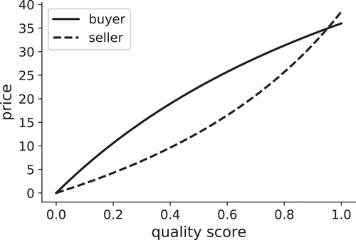
Our application focuses on the London housing market. During the sample period, the London housing market was dominated by sellers (i.e., a sellers’ market), meaning that buyers rarely pay less than their reservation price, as there is so much demand that they need to compete with other buyers.⁹ Hence, we assume that the agreed price is the bid, i.e., the maximum that the buyer is willing and can pay.

Implementation

Table 1 presents the model parameters and indicates the data source from which they are obtained. The free parameters of the model are the latent quality factors ${\phi }_1,\dots ,{\phi }_H$, which we calibrate in the next section. All other parameters are obtained from the data.

Table 1. Parameters and data source.

Parameter	Concept	Data source
$\mathit{N}$	number of agents	Wealth and Assets Survey
$\mathit{H}$	number of properties	Energy Performance Certificate
${\alpha }_i$	consumption/labour preferences	estimated as in (Guerrero, 2020)
${\beta }_i$	housing preferences	estimated as in (Guerrero, 2020)
$\mathit{\gamma }$	discount rate	ONS Annuity Rates and Discount Factors
$\mathit{\delta }$	survival probability	UK National Life Tables
$w_i$	wage	Wealth and Assets Survey
$B_i$	non-labour income	Wealth and Assets Survey
$s_i$	government transfers	Wealth and Assets Survey
$1-{\tau }_i$	labour income tax	Wealth and Assets Survey
$1-z_i$	non-labour income tax	Wealth and Assets Survey
${\phi }_k$	latent quality factor	calibrated according to subsection 3.2

Notes: Parameter ${\alpha }_i$ is estimated according to the identity ${\alpha }_i=\frac{c_i}{{\tau }_i{w}_i{\mathrm{\ell }}_i+c_i}$, following (Guerrero, 2020). Parameter ${\beta }_i$ is estimated according to the identity $\mathit{\beta }=\frac{p}{p+{\mu }_L\mathit{Q}(\mathit{\tau w}+\mathit{zB}+\mathit{s})}$, following (Guerrero, 2020).

We implement the model computationally by instantiating a population of agents representing households (at a one-to-one scale with London) and properties (the data capture approximately 35% of London’s real estate). The initial property ownership is allocated at random. The agents can trade within their lifespan and are replaced by new agents who inherit their property portfolios. After several iterations, the market reaches a steady state with a stable spatial price structure. Algorithm 1 provides further details on the protocol that the model follows.

Algorithm 1: Agent-computing model.

Input: $\{\mathit{N},\mathit{H},B_i,w_i,{\tau }_i,z_i,s_i,{\alpha }_i,{\beta }_i,\mathit{\delta },\mathit{\gamma }\}$ for every agent $\mathit{i}$

1. foreach time step $\mathit{t}$ do

2. foreach agent $\mathit{i}$ do

3. increase age;

4. survive with probability ;

5. if agent dies then

6. reset age;

7. foreach property-search round do

8. match agent to property $\mathit{k}$; ;

9. produce a bid $p_{\mathit{i},\mathit{k}}$ and send it to the owner of $\mathit{k}$;

10. sort properties from the most to the least profitable;

11. foreach property $\mathit{k}$ do

12. owner $\mathit{j}$ produces an ask price $p_{\mathit{j},\mathit{k}}$;

13. if the highest bid is $p_{\mathit{i},\mathit{k}}>p_{\mathit{j},\mathit{k}}$ then

14. transact property;

15. update property portfolios;

16. remove any offer that buyer $\mathit{i}$ may had made on other properties

Data, calibration, and validation

Data

Households

The household data are the same used in Guerrero (2020), with the main source being the UK’s Wealth and Assets Survey (WAS), conducted by the Office of National Statistics (ONS) on a biannual basis. We use the fifth wave of the WAS (from July 2014 to June 2016).¹⁰ For population-level variables such as the discounting factor and the survival probability, we use ONS Annuity Rates and Discount Factors dataset, and the National Life Tables respectively. Both datasets cover the same sampling period as the WAS. Table 1 explains how $\mathit{\alpha }$ and $\mathit{\beta }$ are calculated from the WAS dataset using microeconomic identities. In Table 2, we provide the summary statistics of the household data.

Table 2. Summary statistics of the variables obtained from the wealth and assets survey.

Variable	Symbol	Mean	Standard deviation
Number of households	$\mathit{N}$	3,344,438	-
Wage	$\mathit{w}$	£37,324.02	£62,083.05
Non-labour income	$\mathit{B}$	£1755.18	£19,203.72
Government transfers	$\mathit{s}$	£401.09	£1465.02
Labour-income tax	$1-\mathit{\tau }$	22.19%	12.82%
Non-labour income tax	$1-\mathit{z}$	0.63%	4.47%
Age (of household head)	$\mathit{L}$	47.13 years	11.56 years
Consumption/labour preference	$\mathit{\alpha }$	0.27	0.1
Housing preference	$\mathit{\beta }$	0.69	1.49

Notes: All monetary variables are in an annual basis.

Properties

We construct two property datasets following similar procedures as the ones applied by Law et al. (2019) and Chi et al. (2021). The first one consists of the London price-paid data for 2016, which contains the transaction price, property attributes, and the predicted price for 71,831 transactions (representing 95% of all property transactions in London in 2016). In Table 3, we provide the summary statistics of this dataset. The second source is the London property data, which contain 1.2 million properties with attributes (representing 35% of all properties in London). In Table 4, we provide the summary statistics for the London property data. Five sources of data are used to compile the two property datasets:

Table 3. Summary statistics of the 2016 London price-paid data.

Variable	Count	Mean	std	min	25%	50%	75%	max
lnprice	71,831	12.98	0.53	8.87	12.67	12.95	13.28	15.10
quality rail	71,831	21.74	9.72	3.20	15.18	19.58	25.70	95.79
quality cross	71,831	21.99	9.79	3.20	15.39	19.84	25.98	95.79
railtime	71,831	54.02	24.58	3.67	36.41	49.07	66.79	165.41
crosstime	71,831	51.12	21.91	3.67	35.02	47.75	63.57	151.10
size	71,831	84.05	35.98	11.97	59.00	77.00	100.00	249.50
type	71,831	0.55	0.50	0.00	0.00	1.00	1.00	1.00
age	71,831	0.28	0.45	0.00	0.00	0.00	1.00	1.00
retail	71,831	8.63	10.93	1.00	2.00	5.00	11.00	99.00
office	71,831	2.57	4.64	1.00	1.00	1.00	2.00	74.00
amenity	71,831	152.82	168.66	1.00	49.00	95.00	192.00	2674.00
parks	71,831	1.46	1.40	0.69	0.69	0.69	1.81	6.86
Predict rail	71,831	12.98	0.43	10.14	12.70	12.93	13.21	14.86
Predict cross	71,831	13.00	0.43	10.18	12.72	12.95	13.22	14.87

Sources: Land Registry, Ministry of Housing, Communities and Local Government, Ordnance Survey, open street maps, Historic England.

Table 4. Summary statistics of the London property data.

Variable	Count	Mean	std	min	25%	50%	75%	max
quality rail	1,235,194	20.29	9.71	3.27	13.92	18.20	24.01	155.30
quality cross	1,235,194	20.56	9.79	3.32	14.13	18.47	24.34	155.30
railtime	1,235,194	48.74	25.67	2.84	30.28	42.33	60.02	224.17
crosstime	1,235,194	45.60	22.21	2.84	28.85	40.80	57.50	207.94
size	1,235,194	75.79	34.54	15.01	51.60	69.32	90.18	249.99
type	1,235,194	0.47	0.50	0.00	0.00	0.00	1.00	1.00
age	1,235,194	0.38	0.48	0.00	0.00	0.00	1.00	1.00
retail	1,235,194	12.76	14.09	1.00	3.00	7.00	17.00	100.00
office	1,235,194	3.68	6.46	1.00	1.00	1.00	4.00	75.00
amenity	1,235,194	224.61	226.67	2.00	64.00	146.00	316.00	2746.00
parks	1,235,194	0.74	0.38	0.69	0.69	0.69	0.69	6.86
predicted rail	1,235,194	12.94	0.44	9.97	12.66	12.90	13.16	15.02
predicted cross	1,235,194	12.96	0.43	9.97	12.68	12.91	13.18	15.02

Sources: Ministry of Housing, Communities and Local Government, Ordnance Survey, open street maps, Historic England.

(1) the Land Registry price-paid dataset, which contains the price paid for each property in London; (2) the Ministry of Housing, Communities and Local Government Domestic Energy Performance certificate data, containing the property structural attributes such as the size, the number of bedrooms, the dwelling age and the dwelling type;

(3) the Ordnance Survey road network data, used to compute the accessibility measures for the quality score;

(4) the Open Street Maps land use data, used to compute access to neighbourhood amenities measures;

(5) the Historic England Parks and garden data, used to compute access to greenery measures.

In order to fully exploit the data in the London property dataset, we need to estimate prices for dwellings that do not appear in the price-paid dataset (because they were not transacted). Thus, we predict the house price for the London property dataset by training an Extra Gradient Boosting Regressor (Xgboost) (Chen & Guestrin, 2016) on the subset of properties that appear in both datasets. Specifically, we sample 67% of the data for training and 33% of the data for testing. The trained Xgboost model predicts log-prices and achieves an out-of-sample $R^2$ of 70%.¹¹

Calibration

The model requires calibrating $\mathit{H}$ parameters, one per property. These correspond to the latent quality factors ${\phi }_1,\dots ,{\phi }_H$. The latent quality factors help linking the subjective valuation of the agents with the objective features of properties. Since ${\phi }_k$ influences the price at which property $\mathit{k}$ may be traded at a given point in time, the objective of the calibration is to find a set $\{{\phi }_1,\dots ,{\phi }_H\}$ such that the average price of each property – in the steady state – is matched to its empirical counterpart. To achieve this, we implement a multi-output gradient descent algorithm that simultaneously explores the full parameter space and minimises the error function describing the average price discrepancy. Such procedure was developed by Guerrero and Castañeda (2020) and refined in Guerrero et al. (2023). This algorithm has been successfully used to calibrate high-dimensional agent-computing models where each evaluation is computationally expensive. Two virtues of this method are that all parameters are adjusted simultaneously (for efficiency), and that the calibration is direct, so no surrogate models are necessary (a common strategy with large agent-computing models). In this section, we explain this algorithm and show that it yields an excellent performance.

Let us define the calibration error as the average absolute difference between the empirical and the simulated property prices. Formally, this is

(10) $\mathit{\epsilon }=\frac{1}{H}\sum _{\mathit{k}=1}^H|p_k-{\hat{p}}_{\mathit{k}}|,$(10)

where $p_k$ is the empirical price of property $\mathit{k}$ and ${\hat{p}}_{\mathit{k}}$ is the one (steady-state average) produced by the model. The simulated price ${\hat{p}}_{\mathit{k}}$ is the average price at which property $\mathit{k}$ was sold across a set of independent Monte Carlo simulations. To collect ${\hat{p}}_{\mathit{k}}$, we need to (1) make sure that the simulation has reached its steady state and (2) that we run enough Monte Carlo simulations. For the application to the London housing market, we find that the model reaches the steady state after 100 iterations, so we run it for 200 steps and collect the last trading prices. A steady state is achieved when the price index proposed by Guerrero (2020) stabilises.¹² We also find that 100 Monte Carlo simulations are sufficient to obtain ${\hat{p}}_{\mathit{k}}$ with enough precision for the purpose of calibration.

The calibration algorithm adapts every latent factor simultaneously as the information about the property-specific errors is updated. First, after the Monte Carlo simulations are run, we compute ${\epsilon }_k=|p_k-{\hat{p}}_{\mathit{k}}|$. If $p_k>{\hat{p}}_{\mathit{k}}$, then we update ${\phi }_k$ by multiplying it by $1+({\epsilon }_k/p_k{)}^4$. If, on the other hand, $p_k>{\hat{p}}_{\mathit{k}}$, then we multiply ${\phi }_k$ by $1-({\epsilon }_k/p_k{)}^4$. This procedure enables changes in ${\phi }_k$ that are sufficiently small to bring ${\hat{p}}_{\mathit{k}}$ closer to $p_k$. Repeating these steps gradually reduces the error. Higher precision (and hence a smaller error) can be achieved with more Monte Carlo simulations (at the cost of computational time).

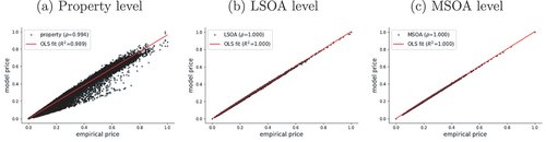
Figure 2 shows the results of the calibration. Panel (a) presents the correspondence between the empirical prices and the ones generated by the model, for each individual property in the dataset. These prices have been generated by the economic behaviour of the agents, who react to the quality of the properties and interact with each other. While the mean error is minimised, perhaps more meaningful measures to assess the fit are the linear correlation coefficient ($\mathit{\rho }$) and the $R^2$ of a linear fit between the empirical dataset and the simulated one. Both metrics confirm an excellent fit at a highly disaggregated level. When aggregating the simulated and the empirical prices at the level of Lower Layer Super Output Areas (LSOA) and Middle Layer Super Output Areas (MSOA) the fit improves considerably.

Figure 2. Model calibration and match to empirical data at different aggregation levels.

Notes: The model is calibrated at the level of each individual property by finding the latent quality factor of the quality score that minimises the price error. In panel (a), each dot represents the average last price of 100 Monte Carlo simulations. Panels (b) and (c) are aggregations of panel (a) made by averaging the property prices within each geographical unit. All the variables in the panels have been re-scaled between 0 and 1 using the popular min-max normalisation formula.

Validation

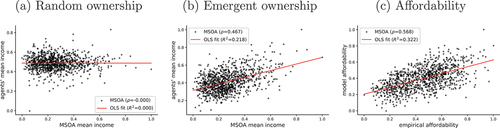
We validate the model by using independent income data, reported at the MSOA level of London (more disaggregated data are not available). These data come from the Family Resources Survey (FRS), which consists of annual reports about household income in the UK. We use the data from the fiscal year ending in 2016 to be consistent with the other datasets. In the model, we do not impose any location to the agents but, instead, initialise a random ownership setup and let them interact so that the most valuable properties are eventually acquired by those who can afford them. Thus, if our theory is valid, the agents should flock to areas where they can afford properties, generating a spatial income distribution similar to that of the FRS dataset. Notice that one should not expect a perfect correlation, as the FRS and the WAS are different types of surveys with different levels of representativeness. Nevertheless, some significant correlation to an independent dataset should be expected from any theory that aims at explaining the housing price structure. The specific variable that we use is gross annual income from the FRS and, for the model, the total income extracted from the WAS.

Figure 3 presents the result of our validation exercise. First, in panel (a), we show the relationship between the MSOA incomes and the average agent income from the model under its initial conditions of random ownership (before allowing the agents to interact). Clearly, under a random assignment, there is no discernible relationship, so the household data do not have an inherent feature that would induce a correlation. Panel (b), in contrast, shows the same variables after running the model. A positive and significant relationship becomes evident, suggesting that the behavioural and interaction mechanisms of the model constitute a valid explanation of how prices emerge. As an additional validation, it is interesting to observe a similarity with respect to the MSOA-level affordability presented in panel (c). Affordability is defined as the ratio of the average income to average property price.

Figure 3. Model validation through the income demographics.

Notes: All the variables in the panels have been normalised between 0 and 1.

These results are important not only for the external validation of the model, but also for its usability in a policy context. In contrast with frameworks where prices are the only dependent variable, our approach also generates endogenous demographic dynamics, such as the spatial distribution of households with different income levels across London, which translates into affordability. Hence, the model can be used for counterfactual analysis to study changes in prices and demographic features. The latter can be highly relevant for the planning and provision of public services by local authorities. In the next section we demonstrate this capability by analysing the potential impact of a new rail line.

Analysing the potential impact of public transport infrastructure

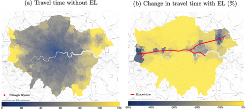
The EL is a major railway infrastructure project that would link London Heathrow airport in the west with Oxford Street, Canary Wharf, Stratford, and Romford in the East. The project is expected to reduce travel time to Central London along the east-west corridor.¹

To obtain the expected time reductions, we deploy two transport network models: a baseline network model and a baseline+EL network model. The baseline network includes the street network, the London Underground, the London Overground, the National Rail within London, the Docklands Light-rail, and the Tramlink. The baseline+EL network model includes all the links from the baseline model plus the EL links. We only include the railway links within the Greater London Authority boundary. These models were kindly provided by Po Nien Chen (P. N. Chen & Karimi, 2018) and we adjusted them for this analysis.

We use these models to calculate the time travel between properties and the CBD. To simplify these calculations we assume the speed of each street link to be 5kph, each rail-base transport links at 33kph, and each EL link at 60kph.¹³ These metrics are the property-specific distances used in the quality score described in Equation 1(1) $q_k={\phi }_k\times \mathit{siz}{e}_k/\mathit{traveltim}{e}_k,$(1) . Figure 4 shows the travel times from the baseline model and the percentage reduction in travel time with the baseline+EL model. The travel time benefits is most obvious in the suburbs to the east and the west of London.

Figure 4. Changes in travel time due to the Elizabeth Line construction.

Notes: The geographical units denoted in the maps represent MSOAs.

Counterfactual design

Our experiment consists of a “control” simulation and a “treatment” one. The treatment is the construction of the EL. The control is the simulation set from the calibrated model as the sample period does not reflect this infrastructure project in the data. To implement the treatment, we compute a new set of observable quality components in the property quality scores. Since the observable quality component accounts for the distance between each property and the CBD (Trafalgar Square), the potential time savings produced by the new line translate into updated quality scores. We assume that the main change to property qualities is precisely the observable component, while the calibrated latent factors remain unchanged. Thus, the treatment or counterfactual consists of running the model with a new set of quality scores that have been impacted through the new distances to the CBD. We analyse the impact of the EL project in terms of price spatial responses and affordability.

Price response

First, let us look at property-specific price changes. Panel (a) in Figure 5 shows the price response function from changes in the quality scores. As expected, we observe a positive relationship between quality and price changes. Price changes seem to respond non-linearly to quality shifts; they exhibit a clear positive trend in the first third of the quality range, and then reach a plateau at higher quality levels.

Figure 5. Price responses to changes in property quality.

Notes: Each data point is obtained by computing the average level of the relevant variable across 100 Monte Carlo simulations. Price and quality changes are computed as: $100\times (\mathit{predictedValue}-\mathit{baseValue})/\mathit{baseValue}$.

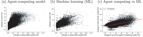
An interesting exercise is comparing the outcome of these counterfactuals against the predictions made by the machine-learning (ML) model trained in the price-imputation step. Panel (b) shows the resulting response function. First, the ML estimation is qualitatively consistent with our model results, providing further validity to our approach. Second, notice that the ML model suggests a more linear response to quality changes. Third, while panel (a) shows a price-change volatility that decays with the change in quality, this is not the case in panel (b). Furthermore, the predictions from the ML model seem to be one order of magnitude higher than those from the agent-computing model. We confirm this in panel (c), where we plot the prediction of each property across both models. This graphic shows that the ML approach systematically overestimates the price changes generated by the agent-computing model (most dots lie above the 45-degree line); although there are also groups of properties with underestimated responses. Arguably, these differences between model outcomes are due to the behavioural and institutional micro-mechanisms that are explicit (and validated) in the agent-computing model. This highlights the importance of specifying models with micro-foundations that provide the causal basis of the data-generating process.

Next, let us aggregate the results to the MSOA level in order to study the spatial distribution of price responses. Panels (a) and (b) in Figure 6 show the response functions aggregated at the MSOA level. The difference in price-change volatility between both types of models is preserved when we aggregate the data. When results are aggregated, the difference in the magnitude of price changes goes away. The spatial aggregation result is not surprising and is known in geography as the modifiable areal unit problem. Nevertheless, even at the MSOA levels, both models exhibit noticeable differences. Next, we analyse these differences spatially.

Figure 6. Aggregate and spatial price response functions (MSOA level).

Notes: Each data point is obtained by computing the average level of the relevant variable across 100 Monte Carlo simulations.

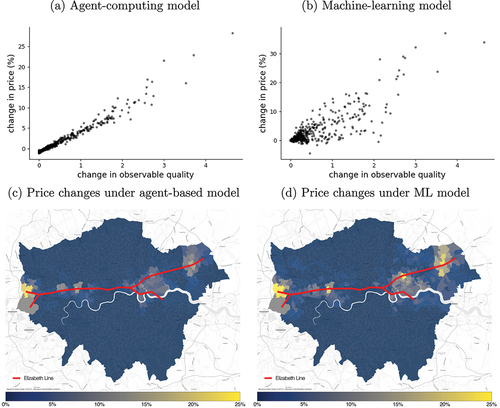
Panel (c) in Figure 6 shows the spatial outcomes under the agent-computing model. The first point to note is that price changes are not uniformly nor smoothly distributed along the EL. Certain neighbourhoods exhibit a stronger positive price effect, for example, West Drayton, Acton, Ealing, Canary Wharf, Stratford, Forest Gate and Romford ($10+\mathrm{\%}$). On the other hand, some stations experience a milder effect, for example, Bond Street in Central London. A second point to note is that the positive price effect diffuses to the surrounding neighbourhoods. For example, the positive price effect from Canary Wharf spreads southwards towards Greenwich which is a neighbourhood connected by the Docklands Lightrail network.

In panel (d), we present the spatial distribution of price changes using the machine learning model. While the overall spatial pattern resembles that of the agent-computing model, there seem to be more neighbourhoods with a high price change than in the agent-computing model (more areas with a stronger yellow tone). Some of these areas are West Drayton and Acton in the west and Forest Gate and Romford in the east ($20+\mathrm{\%}$).

Affordability

One of the key advantages of our modelling approach is the ability of matching – through sound socioeconomic theory – demographic and property data that are difficult to obtain on the scale of this study. As we have shown, the model is flexible to accommodate different types of agent-level attributes such as age and income. Since the mechanisms of the model are mainly economic, we focus on the interaction between income and home ownership.¹⁴

Affordability is measured as the ratio of household income to property price. From a static point of view, it tells us how much a household’s income represents in terms of the property equity. From a dynamic perspective, measuring changes in affordability is important for urban planning because they provide information about potential demographic shifts in a given area. For example, if affordability worsens, it means that those agents who leave an MSOA are less likely to be replaced by “similar” households – in terms of income – and this implies a demographic recomposition; perhaps lower income diversity. A demographic recomposition, in turn, may demand updating the provision of public services. In this section, we are mainly concerned about this dynamic view of affordability, so we study how the new EL would affect it.¹⁵

First let us consider the simultaneous changes in prices and income of property owners due to the EL. A trivial outcome would be that both variables move in unison, for example, that wealthier agents almost always buy the properties that experience price surges. Panel (a) in Figure 7 suggests that this is not the case since we observe both positive and negative income changes that correspond to price increments. As indicated by the colour gradient, most of these co-movements concentrate in smaller percent changes (around the zero-zero coordinate). Nevertheless, large price changes also exhibit both positive and negative income changes.

Figure 7. Elizabeth-line-induced affordability changes (property level).

Notes: Each data point is obtained by computing the average level of the relevant variable across 100 Monte Carlo simulations. The color gradient indicates density or higher frequency, with the red tones denoting higher levels.

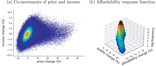
Next, let us analyse how affordability responds to changes in the observable quality of the properties. Panel (b) presents a histogram (with frequencies in logarithmic scale) of the different combinations between quality changes and affordability changes. We can obtain some interesting insights from this graphic. First, on average, affordability decreases with larger changes in the quality of properties. Thus, those areas that benefit the most from the new infrastructure could experience a demographic recomposition. Second, while the association of affordability with respect to quality changes is negative, there is a substantive amount of properties that would experience a positive change in affordability (those in the upper corner of the plot). In fact, these properties amount to approximately 46% of all the real state in the model. From a planning perspective, these areas should receive attention as they are expected to receive an inflow of households with a different income structure from that of the current residents, so evaluating whether the current public services in those areas would satisfy the new residents should be important.

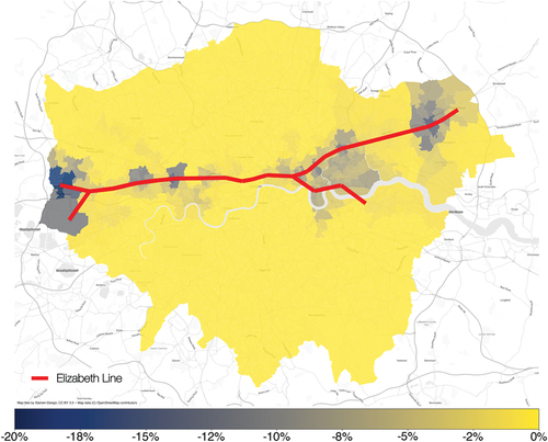
Figure 8, presents the spatial distribution of affordability changes. Similar to the price response differences, the areas that are less affordable are those that have greater increase relative to its income. Suburban areas such as West Drayton and Acton have a greater reduction in affordability ($10+\mathrm{\%}$) than Central London. On the other hand, areas in East London such as Canary Wharf, Stratford, Forest Gate, and Romford also exhibit a notable reduction in affordability. The suppressed effect of both price and affordability in Central London is less intuitive and could be attributed to Central London’s exceedingly rich infrastructure that gets richer comparatively less to the outlying areas. This interesting and less intuitive insight shows the benefit of an agent-computing approach, as it allows policy makers to be inquisitive about the factors that endogenously change within the model. In this case, we are able to study the effect that transport innovation has on income and affordability, which has important societal impact and implications.

Figure 8. Spatial distribution of changes in affordability (MSOA level).

Discussion and conclusion

Foreseeing demographic changes and shifts in the demand of public services is one of the biggest challenges that urban planners have to face. Often, these dynamics are driven by behavioural responses to price changes that are triggered by major infrastructure investment. Sometimes, properties that experience a price surge will attract wealthier households. Others, they will spark a demographic reconfiguration through the regional flock of mixed-income households. These changes are difficult to predict because, for example, they are non-linear and non-monotonic; they obey to behavioural responses that are not identifiable in house price datasets; and they require a combination of property and demographic data that is rare or difficult to obtain due to data privacy, at least in publicly available sources. In this paper, we develop an agent-computing model that helps overcome some of these challenges and provides a robust tool for the ex-ante estimation of policy impacts in the housing market.

A novelty of this research is comparing the differences between the outputs of an agent-computing model and a machine learning model, where the former explicitly models the housing transaction processes while the latter is a black-box to predict dwelling prices. The result shows that the two approaches can be complementary in capturing largely similar spatial patterns. However, they also suggest the agent-computing approach is able to provide additional insight and interpretable evidence in terms of income and affordability.

This brings upon a second novelty of the research: combining traditional micro-economic theory and agent-computing with highly granular spatial data. Being able to model explicit social mechanisms and to predict prices, income, and demographics simultaneously in space gives policy makers and planners greater transparency to examine different policy levers and factors for anticipating future cities.

These contributions do not come without limitations. First, as with all models, some assumptions may not hold in every specific context (e.g., with the mega-wealthy buyers). Second, the model may not be able to correctly predict long-term trends as the necessary data to train it would most likely experience structural changes. Third, the model is designed to work with large-scale data on properties and households, which may not be available in many countries or regions. Fourth, our travel-time accessibility metric, captures more nuanced aspects of accessibility compared to conventional distance-to-CBD measure. We acknowledge, however, that there are additional spatial factors not entirely accounted for. As a result, future research will explore further these spatial aspects of housing quality, including its spatial configurations and neighbourhood amenities. While these limitations constrain the generalisability of the model, they are common in most models, so we believe that they do not invalidate of demerit the contributions made in this paper. Instead, they point out to potential new research avenues to make this framework accessible to a broader research community.

In terms of potential implications of our findings, various policy interventions may come to mind in order to address the potential emergence of affordability issues. While assessing the impact of such interventions lies beyond the scope of this paper, we can briefly discuss the relevance of some policy instruments and the adjustments that would be required in the model to test them. First, there is the instrument of council tax, which could be adjusted by the local authorities base on household income. From the point of view of the model, this is easy to do as one only needs to add a term to the budget constraint equation of the agents that specifies the level of council tax. Hence, a potential follow-up project could consist of incorporating spatial data on council taxes and seeing what would be the wealth effects of different interventions. Second, social transfers could be implemented in similar way as a council tax intervention. In terms of real-world implementation, both types have challenges regarding identifying the target population, and dealing with potential conflicting objectives in terms of the local authorities public spending strategies.

To conclude, this study proposes a process-base computational framework to study highly granular geographically-explicit policy recommendations. Some of the natural extensions that will follow this framework are the incorporation of a rental market, of financial instruments, and of social housing. All of these are key aspects of housing markets that should be properly understood under the umbrella of an integrated analytical framework like the one we propose here.

Data and codes availability statement

The code that support the findings of this study is available here https://github.com/oguerrer/LHM/.

Acknowledgments

The authors thank Po Nien Chen from UCL for sharing with us the network model for calculating the travel time accessibility.

Disclosure statement

No potential conflict of interest was reported by the author(s).

Additional information

Funding

This work was supported by the Economic and Social Research Council.

Notes

1. The main sections of the EL network opened in 2022.

1. data.london.gov.uk/dataset/average-house-prices

2. In urban economics, it has been pointed out that Alonso’s bid-rent theory is a simplistic model with well-known limitations such as its monocentric assumption. Despite this and other related criticisms, the core principles of this canonical theory remain largely relevant in the literature (e.g., residential land values arise from a trade-off between accessibility and commuting cost). Furthermore, there seems to be new empirical evidence suggesting that this theory performs satisfactorily when adapted to the modern context where price gradient can be explained by employment accessibility (Ahlfeldt, 2011).

3. An alternative approach to match micro-level data in a spatial setting is spatial micro-simulation (Tanton, 2013). While this framework is useful to produce matches based on probabilistic associations between variables, it lacks the behavioural foundations of why people choose to live in specific areas. These foundations are critical to estimate the impact of policy interventions. Hence, micro-simulation is ill-equipped to produce relevant counterfactuals.

4. While London has a significant number of employment centres outside Central London, most workplaces in the city are located in Inner London. Previous research has shown that, within Inner London, the distance or travel time to the CBD still captures most of the variance produced through more complex accessibility measures such as the gravitational potential to employment centres used in hedonic price models (Ahlfeldt, 2011; Law et al., 2013).

5. A more complex functional form (i.e., exponential) can be applied on the travel time impedance in the denominator. We find that this does not change our results significantly.

6. A buyer may visit multiple properties before providing a bid, in which case they send it to the property that generates most utility through the potential growth of the buyer’s portfolio (see Equation 4). A seller, on the other hand, may receive multiple offers and pick the best one.

7. O. A. Guerrero (2020) shows that this specification is consistent with empirical evidence on the myopic financial planning of households when it comes to housing consumption; providing the foundations of a realistic theoretical framework.

8. Note that the reservation price is endogenous. This is an important advantage over many housing market models since they need to exogenously assume a reservation price structure, something unobservable in real world data.

9. Even after the Covid pandemic, while having high interest rates, journalistic evidence suggests that the London housing market is still heavily influenced by sellers.

10. While the WAS consists of a sample of British households, it is possible to use the variables’ weights to generate a synthetic population matching the more than 3 million households in London. These weights are already corrected for sampling biases.

11. Xgboost is a very popular and state-of-the-art machine learning algorithm for modelling tabular data (Shwartz Ziv & Armon, 2022). Throughout the paper, we use the terms Xgboost model and “machine learning model” interchangeably. Specifically, we use the xgboost library in Python and tune the number of decision trees as a hyper-parameter ( = 500).

12. The procedure to construct the price index consists of creating an “average” agent, i.e., a synthetic household with the average characteristics of London households. This agent approaches each homeowner and offers a bid for each one of their properties. Hypothetical transaction prices are produced in each one of these encounters following the specification described in sec:model_households. The price index is the average of these elicited prices.

13. The assumed speed of the EL link is slower than the highest speed to ensure we are not overestimating its benefits.

14. The model can easily take into account demographic traits such as age, class, ethnicity, and occupation since the WAS contains such variables. However, it would be disingenuous to analyse the impact on these features since our social mechanisms are mainly economic. Further work should try to incorporate social processes where characteristics such as race affect housing market transactions.

15. Importantly, while we are able to compare the price-response functions produced by the agent-computing and the ML models, this is not feasible with affordability, at least not at the property level. This is so because machine learning needs a training dataset where households are matched to properties.

References

- Ahlfeldt, G. (2011). If Alonso Was Right: Modeling accessibility and explaining the residential land gradient. Journal of Regional Science, 51(2), 318–338. https://doi.org/10.1111/j.1467-9787.2010.00694.x
- Alonso, W. (1964). Location and land use: Toward a general theory of land rent. Harvard University Press.
- Anacker, K. B. (2019). Introduction: Housing affordability and affordable housing. International Journal of Housing Policy, 19(1), 1–16. https://doi.org/10.1080/19491247.2018.1560544
- Arthur, W. B. (1999). Complexity and the economy. Science, 284(5411), 107–109. https://doi.org/10.1126/science.284.5411.107
- Axtell, R. L. (2007). What economic agents do: How cognition and interaction lead to emergence and complexity. The Review of Austrian Economics, 20(2), 105–122. https://doi.org/10.1007/s11138-007-0021-5
- Baptista, R., Farmer, D., Hinterschweiger, M., Low, K., Tang, D., & Uluc, A. (2016). Macroprudential policy in an agent-based model of the UK housing market. Working Paper 619, Bank of England.
- Batty, M. (2007). Cities and complexity: Understanding cities with cellular automata, agent-based models, and fractals. The MIT press.
- Cao, S. (2021a). Why zillow’s home-flipping business is doomed to fail—expert weighs in.
- Cao, S. (2021b, November 10). Zillow’s Fixer-Upper Disaster: Why Zestimate Couldn’t Get Home Pricing Right. Observer. https://observer.com/2021/11/zillow-zestimate-predict-home-price-wrong-ibuying-shutdown/
- Chen, T., & Guestrin, C. (2016). XGBoost: A Scalable Tree Boosting System. Proceedings of the 22nd ACM SIGKDD International Conference on Knowledge Discovery and Data Mining, San Francisco, California, USA (pp. 785–794).
- Chen, P. N., & Karimi, K. (2018). The impact of a new transport system on the neighbourhoods surrounding the stations: The cases of Bermondsey and west ham, London. 24th ISUF 2017 - City and Territory in the Globalization Age. https://doi.org/10.4995/ISUF2017.2017.5971
- Cheshire, P., & Sheppard, S. (1995). On the price of land and the value of amenities. Economica, 62(246), 247. https://doi.org/10.2307/2554906
- Chi, B., Dennett, A., Oléron-Evans, T., & Morphet, R. (2021). Shedding new light on residential property price variation in England: A multi-scale exploration. Environment and Planning B: Urban Analytics and City Science, 48(7), 1895–1911. https://doi.org/10.1177/2399808320951212
- Dieci, R., & Westerhoff, F. (2012). A simple model of a speculative housing market. Journal of Evolutionary Economics, 22(2), 303–329. https://doi.org/10.1007/s00191-011-0259-8
- Edwards, M. (2016). The housing crisis and london. City, 20(2), 222–237. https://doi.org/10.1080/13604813.2016.1145947
- Ehrenhalt, A. (2012). The great inversion and the future of the American city. Vintage.
- Erlingsson, E., Raberto, M., Stefánsson, H., & Sturluson, J. (2013). Integrating the housing market into an agent-based economic model. In A. Teglio, S. Alfarano, E. Camacho-Cuena, & M. Ginés-Vilar (Eds.), Managing market complexity: The approach of artificial Economics, lecture notes in economics and mathematical systems (pp. 65–76). Springer.
- Erlingsson, E., Teglio, A., Cincotti, S., Stefansson, H., Sturlusson, J., & Raberto, M. (2014). Housing market bubbles and business cycles in an agent-based credit economy. Economics: The Open-Access, Open-Assessment E-Journal, 8(2014–8), 1–42. https://doi.org/10.5018/economics-ejournal.ja.2014-8
- Filatova, T., Parker, D., & Veen, A. (2009). Agent-based urban land markets: Agent’s pricing behavior, land prices and urban land use change. Journal of Artificial Societies and Social Simulation, 12, 1–3.
- Gallent, N., Durrant, D., & May, N. (2017). Housing supply, investment demand and money creation: A comment on the drivers of London’s housing crisis. Urban Studies, 54(10), 2204–2216. https://doi.org/10.1177/0042098017705828
- Gan, Q., & Hill, R. J. (2009). Measuring housing affordability: Looking beyond the median. Journal of Housing Economics, 18(2), 115–125. https://doi.org/10.1016/j.jhe.2009.04.003
- Ge, J. (2014). Who creates housing bubbles? An agent-based study. In S. Alam & H. Parunak (Eds.), Multi-agent-based simulation XIV, lecture notes in computer science (pp. 143–150). Springer.
- Ge, J. (2017). Endogenous rise and collapse of housing price: An agent-based model of the housing market. Computers, Environment and Urban Systems, 62, 182–198. https://doi.org/10.1016/j.compenvurbsys.2016.11.005
- Geanakoplos, J., Axtell, R., Farmer, J., Howitt, P., Conlee, B., Goldstein, J., Hendrey, M., Palmer, N., & Yang, C. (2012). Getting at systemic risk via an agent-based model of the housing market. American Economic Review, 102(3), 53–58. https://doi.org/10.1257/aer.102.3.53
- Gibbons, S., & Machin, S. (2005). Valuing rail access using transport innovations. Journal of Urban Economics, 57(1), 148–169. https://doi.org/10.1016/j.jue.2004.10.002
- Gibbons, S., & Machin, S. (2008). Valuing school quality, better transport, and lower crime: Evidence from house prices. Oxford Review of Economic Policy, 24(1), 99–119. https://doi.org/10.1093/oxrep/grn008
- Gilbert, N., Hawksworth J, C., & Swinney J, A. (2009). An agent-based model of the English housing market. In Papers from the 2009 AAAI Spring Symposium, Technical Report SS-09-09, pages 30–35, Stanford, CA, USA.
- Glynn, C., Byrne, T. H., & Culhane, D. P. (2021). Inflection points in community-level homeless rates. The Annals of Applied Statistics, 15(2), 1037–1053. https://doi.org/10.1214/20-AOAS1414
- Guerrero, O. (2020). Decentralized markets and the emergence of housing wealth inequality. Computers, Environment and Urban Systems, 84, 101541. https://doi.org/10.1016/j.compenvurbsys.2020.101541
- Guerrero, O., & Castañeda, G. (2020). Policy priority inference: A computational framework to analyze the allocation of resources for the sustainable development goals. Data & Policy, 2. https://doi.org/10.1017/dap.2020.18
- Guerrero, O., Guariso, D., & Castañeda, G. (2023). Aid effectiveness in sustainable development: A multidimensional approach. World Development, 106256, 168. https://doi.org/10.1016/j.worlddev.2023.106256
- Heppenstall, A. J., Crooks, A. T., See, L. M., & Batty, M. (2011). Agent-based models of geographical systems. Springer Science & Business Media.
- Jeanty, P. W., Partridge, M., & Irwin, E. (2010). Estimation of a spatial simultaneous equation model of population migration and housing price dynamics. Regional Science and Urban Economics, 40(5), 343–352. https://doi.org/10.1016/j.regsciurbeco.2010.01.002
- Kirman, A. P. (1992). Whom or what does the representative individual represent? Journal of Economic Perspectives, 6(2), 117–136. https://doi.org/10.1257/jep.6.2.117
- Kouwenberg, R., & Zwinkels, R. (2015). Endogenous price bubbles in a multi-agent system of the housing market. Public Library of Science One, 10(6), e0129070. https://doi.org/10.1371/journal.pone.0129070
- Law, S., Karimi, K., Penn, A., & Chiaradia, A. (2013). Measuring the influence of spatial configuration on the housing market in metropolitan London. In Proceedings of the Ninth International Space Syntax Symposium, Seoul, Korea (pp. 121–1).
- Law, S., Paige, B., & Russell, C. (2019). Take a Look Around: Using Street View and Satellite Images to Estimate House Prices. ACM Transactions on Intelligent Systems and Technology, 10(5), 1–54. https://doi.org/10.1145/3342240
- McKee, K. (2012). Young people, homeownership and future welfare. Housing Studies, 27(6), 853–862. https://doi.org/10.1080/02673037.2012.714463
- McMahon, M., Berea, A., & Osman, H. (2009). An agent based model of the housing market. Working Paper.
- Meen, G. (2005). On the economics of the barker review of housing supply. Housing Studies, 20(6), 949–971. https://doi.org/10.1080/02673030500291082
- Meen, G. (2011). A long-run model of housing affordability. Housing Studies, 26(7–8), 1081–1103. https://doi.org/10.1080/02673037.2011.609327
- Parker, D., & Filatova, T. (2008). A conceptual design for a bilateral agent-based land market with heterogeneous economic agents. Computers, Environment and Urban Systems, 32(6), 454–463. https://doi.org/10.1016/j.compenvurbsys.2008.09.012
- Piketty, T. (2014). Capital in the twenty-first century. Harvard University Press.
- Rosen, S. (1974). Hedonic prices and implicit markets: Product differentiation in pure competition. Journal of Political Economy, 82(1), 34–55. https://doi.org/10.1086/260169
- Shwartz Ziv, R., & Armon, A. (2022). Tabular data: Deep learning is not all you need. Information Fusion, 81, 84–90. https://doi.org/10.1016/j.inffus.2021.11.011
- Simon, H. A. (1984). On the behavioral and rational foundations of economic dynamics. Journal of Economic Behavior & Organization, 5(1), 35–55. https://doi.org/10.1016/0167-2681(84)90025-8
- Tanton, R. (2013). A review of spatial microsimulation methods. International Journal of Microsimulation, 7(1), 4–25. https://doi.org/10.34196/ijm.00092