Live fitting of process data within digital twins of manufacturing to use simulation and optimisation

ABSTRACT

In production scenarios, uncertainty in production times, and scrap rates is common. Uncertainty can be described by stochastic models that need continuous updates due to changing conditions. This paper models probability distributions and estimates their parameters from real-world data on processing times and scrap rates. It uses live fitting to identify timely changes in the data sets, comparing different distributions. The fitting and live fitting approaches are applied to data from a real production system to compare the goodness of fit for different distributions and to demonstrate the reliability of the reaction to changes in the input data. Data and probability estimations are categorised, and a concept combining simulation and optimisation models is developed to optimise scheduling. The vision of the research presented in this paper is an online approach that determines quasi-optimal schedules for production systems based on current data from the system and its environment.

KEYWORDS:

• Live fitting
• processes fitting
• manufacturing
• scheduling
• combinatorial optimisation
• dynamic optimisation

1. Introduction

In times of increasing digitisation in manufacturing, a large amount of data can be generated. In principle, the more data available, the easier it is to monitor, analyse, and improve processes and parameters on a transparent and controlled basis. An application field for optimisation in manufacturing processes is machine scheduling. Processing times and scrap rates are two influencing parameters for computing schedules. They also include uncertainty but are usually calculated from deterministic models in the first step and are afterwards improved using simulation-based optimisation.

For the second step, besides deterministic models and optimisation algorithms, simulation experiments are used to test such optimisation results under realistic conditions (Bauernhansl, ten Hompel, and Vogel-Heuser, 2014; Law, 2015; Müller et al., 2018; Pinedo, 2016; Schumacher & Buchholz, 2020; Waniczek et al., 2017). However, the resulting schedules are only valid if the parameters of the model, especially the distributions used for modelling stochastic effects, adequately present the real behaviour. Thus, the adequate representation of monitored data in the optimisation model is a key factor in model-based optimisation.

In the following, the characteristics of scrap rates and processing times are analysed in more detail. Scrap rates are rates of defective products in manufacturing that need to be rejected. Scrap data is interesting for optimisation since it represents an uncertainty factor concerning the number of parts produced. Fortunately, an accumulation of scrap rates close to zero is observed in most production processes, and the larger the scrap rate, the less frequently it is usually observed. Processing times are times a machine needs to produce one part of a certain product. Different processing times can occur despite the same machines and the same part being produced. This uncertainty is closely related to the manufacturing process itself and caused by a variety of environmental influences, such as room temperature in the context of heating processes (Schumacher & Buchholz, 2020). Both quantities, scrap rates, and processing times usually show some fluctuation and thus have to be modelled by an appropriate distribution in a simulation model.

In simulation experiments and optimisation runs, data generated from empirical and discrete distributions can be used or theoretical distributions are adapted as models for real data. Since discrete empirical distributions entail disadvantages, like the restriction to measured values and the high effort for storing large sets of data, data is almost always modelled by theoretical probability distributions in stochastic simulations. Theoretical distributions are more robust against outliers, consume less memory, and allow the generation of arbitrarily large data sets. In the first step, deterministic values for optimisation are derived from these distributions (Law, 2015; Schumacher & Buchholz, 2020), and then the detailed distributions are applied in simulation to further improve the resulting schedules.

In times of digitisation, new data are constantly available. It is, therefore, possible and often necessary to develop a process that generates models for live data in real-time (Müller et al., 2018). The permanent availability of new data allows one to improve the stochastic model that represents the data in the simulation model during runtime. This may result in new parameter values or even in another distribution type. These changes have to be considered in the optimisation process. Thus, optimisation may become an online process. As long as data remains homogeneous, changes in the parameters are small, and the optimum will not differ significantly from the previous result. Nevertheless, rescheduling might be necessary due to a change in a parameter or the distribution. More interesting are situations where the data indicates an abrupt change. These critical changes, denoted as change points, have to be detected as soon as possible, resulting in modified parameters of the optimisation model and a recomputation of the optimal schedule. Consequently, techniques for change point detection and recomputation of distribution parameters are required (Buchholz et al., 2019) in a dynamic environment. Available methods for simulation-based optimisation usually do not consider these aspects and assume a model with constant parameters over the whole optimisation process.

The major topic of this paper is the appropriate modelling of scrap rates and processing times of manufacturing processes from real and possibly online data. It analyzes how fitted distributions and their estimations can be used in production planning and machine scheduling by combining simulation and optimisation models. Therefore, statistical distributions are fitted from empirical data and compared, and if possible, an optimal distribution type is selected for each machine type and class of process data, i.e., scrap rates and processing times per machine type. In addition, procedures are developed to identify critical changes in process data, and the effects of the changes to production schedules are to be shown. Methods are evaluated with real data from the manufacturing environment of an automotive supplier. Thus, the paper focuses on the integration of methods to determine distributions from data and integrate these distributions in simulation models for optimisation using available techniques of combining simulation and optimisation.

In Section 2, scheduling problems in industry are characterised. Section 3 shows the state of the art in the literature regarding combining simulation and optimisation models, the handling of production data, outliers analysis for empirical data, fitting and live fitting of empirical production data. Section 4 analyzes the use of fitted distributions and their deterministic parameter estimations in production planning, machine scheduling, and combining simulation and optimisation models. Section 5 concretises the processes to finally estimate distribution parameters for production data. Considering the special texture of data for scrap rates and processing times, procedures for preparing data and parameter estimation are composed. A uniform measure is determined to analyse different model fits, which ensures a valid selection. In addition, a procedure is developed that can automatically analyse and model the entire data set. The live fitting procedure presented in Section 6 uses a data stream consisting of process data from the manufacturing environment to generate a model for the data in real-time. It uses the knowledge gained from previous modelling efforts to develop a streaming algorithm that fits distributions to the live data. It responds dynamically to potential changes in the data situation to ensure an accurate prediction of future system behaviour. To do this, change points in the stream must be detected and handled. The response to such model changes is analysed as a classification problem using metrics designed for this purpose. Section 7 evaluates fitting, live fitting procedures, and implications for production schedules using real data from an automotive supplier. It identified which types of probability distributions fit best for the production environment and how a change in data can influence planning algorithms. In Section 8, the most significant findings of this approach and future research perspective are summarised.

2. Production settings of scheduling problems

Machine scheduling is a central element of a production system to increase its performance and efficiency. Algorithms for scheduling deal with the allocation of jobs to resources or machines. Resources are usually limited, and therefore, jobs compete for them. Machine scheduling aims to realise a schedule that optimises a given criterion (Pinedo, 2016; Ruiz, 2018). Across all industries, time-based objective functions such as the makespan are most commonly used for scheduling problems (Prajapat & Tiwari, 2017). The makespan is defined as the time between the start of the production of the first scheduled job and the latest finishing of the job in the schedule. An exemplary production setup with three machines in stage 1 (M1, M2, M3) and one machine in stage 2, which is used in this paper, is shown in Figure 1. In the first stage, products, for example, are created, and in the second stage, they are further processed, for example, with painting or shaping. All the jobs have the same route to follow through the production flow – first, the first stage, and after that, the second stage. They only need to be processed by one machine per stage.

Figure 1. Production scenario with three machines in stage 1 and one machine in stage 2.

Most combinatorial optimisation problems in operational research and also most scheduling problems are NP-hard (Ruiz, 2018). One approach is to model them as mixed integer problems and solve them with exact algorithms like branch-and-bound. A disadvantage of the exact optimisation methods is the long computation time to reach the optimal or near-optimal solution. For realistic decision problems, it is therefore not possible to plan with exact methods, especially in the case of short-term changes (Clausen et al., 2017; Gendreau & Potvin, 2019).

Heuristic methods are a way to solve complex, realistic decision problems more efficiently. Heuristics are generally defined as methods that provide an approximate solution that is not necessarily proven optimal. They can often achieve better solutions than exact algorithms in a given amount of time (Gendreau & Potvin, 2019; Juan et al., 2015).

The internal and external influencing factors relevant to production planning are subject to an increasingly rapid change. Simulation experiments are used to evaluate machine schedules realistically and integrate stochastic behaviour. However, a simulation run under realistic conditions is costly. Therefore, first, schedules are generated from the deterministic model, and then the best solutions are analysed with simulation experiments (Juan et al., 2015; Schumacher & Buchholz, 2020; Schumacher et al., 2020).

3. Related work

In the following, we review very briefly related work on combining simulation and optimisation models as the basic and above-described optimisation approach, the modelling of production data, outlier detection which is unavoidable in any real setting, and live fitting of data.

3.1. Combining simulation and optimization models

In the area of hybrid flow shop problems, there is a lack of algorithms evaluated on real-world data, and the combination of simulation and optimisation models for such problems is frequently absent in the existing literature (see literature overviews and findings of Fan et al. (2018); MacCarthy and Liu (1993); Morais et al. (2013); Neufeld et al. (2023); Ribas et al. (2010); Ruiz and Vázquez-Rodríguez (2010); Ruiz et al. (2008)). While studies, such as Laroque et al. (2022), have developed simheuristics for hybrid flow shop environments, they have not yet integrated detailed real-world datasets. Complex production scheduling scenarios, like the one conducted by Ruiz et al. (2008), have not combined simulation and optimisation techniques. Initial attempts, as shown by Schumacher and Buchholz (2020), have addressed practical data and implemented a combination of simulation and optimisation, but they have not considered dynamic data adaptation and did not take into account changes in data over time.

Due to the development towards Industry 4.0, simulation can be applied more realistically, and the combination of optimisation methods with simulation models is increasingly found in studies (Prajapat & Tiwari, 2017). There are several ways to use deterministic and stochastic models simultaneously (Balci, 2003; Figueira & Almada-Lobo, 2014; Juan et al., 2015; Kastens & Büning, 2014; Law, 2015).

The question of how metaheuristics (with their deterministic models) can be combined with simulation runs is addressed in more detail by Juan et al. (2015). Juan et al. (2015) call the combination of metaheuristics and simulation “Simheuristics”. For complex problems with stochastic components, simheuristics is probably the most promising approach because a deterministic optimisation often results in a suboptimal solution and optimisation of the stochastic model from scratch is much too costly. In some sense, the technique combines the best of two worlds. However, to be successful, the deterministic model has to guide the optimisation in the direction of the optimum of the stochastic model, and the stochastic model has to describe the real system precisely enough such that the optimum of the model is similar to the optimum of the real system. The techniques we present in this paper contribute mainly to the second point, the modelling quality of the simulation model.

For combining simulation and optimisation, the model assumption is made that the differences between deterministic and stochastic models are minor. With this assumption, it is very likely that solutions with a good objective function value in the deterministic model also have good objective function values in the stochastic model (Juan et al., 2015; Law, 2015). The closeness of deterministic and stochastic models has been shown for various applications from different fields (Juan et al., 2015) but has to be validated for every new case of application. If the deterministic and stochastic model differs too much, then this shows that stochasticity plays an important role, and the precise modelling of data is even more important. To this end, the developments of this paper contribute to establishing the proximity between the stochastic and deterministic models as well as the model and reality.

3.2. Production data

Appropriate modelling of production data is very important for model-based analysis and optimisation. The use of standard distributions, as commonly done in simulation (Law, 2015), is often not sufficient in a real production environment because it is possible that some values occur more frequently than average, and so they cannot reasonably be covered by the standard distribution models. This is especially a common problem when it comes to modelling data sets with a high number of zero observations (Zuur et al., 2009). In extreme value statistics, some methods are known to solve such problems. Previous works have discussed the possibilities of modelling such data by dividing it into sub-models (Min & Agresti, 2002). A good approach is the so-called Two-Part models, which are often used in such problem settings (Duan et al., 1983). Similar procedures can be applied to describe data that is located over multiple accumulation points, which is also a frequently observed problem while working with process data. In these cases, mixed models can be used to describe the data (Frühwirth-Schnatter et al., 2018).

3.3. Outliers

Since outliers are a recurring problem in analysing real process data, their detection is a problem that has been studied in different ways (Shekhar Jha et al., 2021). The methods that can be used to classify outliers depend on the data situation and the concrete use-case (Chandola & Kumar, 2009). Rule-based detection methods are well suited for univariate process data such as scrap rates. These methods are based on statistical approaches that assign a value to each data entry and decide whether it is an outlier or not. A classification method often used in this context is the calculation of the z-score of a data entry (Rousseeuw & Hubert, 2011). However, since not all the data of a process data set lies within a fixed range, such statistical outlier detection methods will reach their limits. In these cases, data-based clustering methods can provide a remedy (Mandhare & Idate, 2017).

3.4. Live fitting from online data

The common way of representing uncertain or stochastic behaviours in simulations is including stochastic distributions (Law, 2015). For the generation and parametrisation of these models efficient methods and powerful software systems are available (Law, 2011; Nahleh et al., 2013). However, if the distributions are computed during the implementation of the simulation model, then they are based on historical data which could be outdated in a highly dynamic environment, as already argued. Thus, parameters of distributions have to be adjusted during the use of the simulation model based on real-time data (Fowler & Rose, 2004). The corresponding methods are less established and rarely used with stochastic discrete event simulation of production systems. If they are used at all, then very simple techniques are usually applied (Goodall et al., 2019; Wang et al., 2011).

However, in statistics, more sophisticated methods are available to estimate stochastic distributions from online data. There are, in principle, two different problems. First, if the observed process remains homogeneous, then the incoming data from the production process can be used to improve the parameters of distributions in the simulation model that is applied to forecast the production process. Parameter estimation of distributions that are used in simulation is often done by maximising the likelihood function using a variant of the expectation maximisation (EM) algorithm (Dempster et al., 1977). Different online versions of the EM algorithm have been proposed (Buchholz et al., 2019; Cappé, 2011; Cappé & Moulines, 2009; Sobhiyeh & Naraghi-Pour, 2020). These algorithms can be applied to improve the parameters of the simulation model between simulation runs based on current data. This is particularly important for the distribution of rare events like failures in the system where a large amount of data is required to obtain reliable estimates. If the behaviour of the production system changes due to internal or external events, then this change point has to be detected in the incoming data, and a new distribution or a distribution with modified parameters has to be used in future simulation runs. Change point detection is well known in data analysis, and different methods have been proposed (Aminikhanghahi & Cook, 2017; van den Burg & Williams, 2020). Thus, an online approach for data-driven simulation modelling consists of a combination of online parameter estimation or parameter improvement and change point detection to generate simulation models that reflect the current state of the production system.

4. Data concept for combining simulation and optimisation models in industry 4.0 production planning

Based on the concept of combining simulation and optimisation models (see Section 3.1), Figure 2 shows the process flow of the developed dynamic machine scheduling process by Schumacher (2023) based on BPMN 2.0 (Shapiro et al., 2011). BPMN 2.0 provides a standardised notation for modelling business processes and workflows, allowing the data concept of the paper to be adapted to solve various optimisation problems by combining simulation and optimisation models. With the notation, it is also possible to adapt the paper’s data concept for other types of optimisation problems and extend it to more complex options of combining simulation and optimisation, such as simheuristics.

Figure 2. Developed framework for combining simulation and optimization models (Schumacher, 2023).

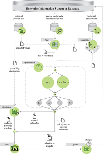
In the upper part of Figure 2, it can be seen that the source of data is the enterprise information system or a(n) (extracted) database. The data in three categories – master and transaction data, historical process data, and historical demand data – form the basis of the process. With the help of a Graphical User Interface (GUI), the data can be analysed with business intelligence tools in more detail by the team, parameters for the optimisation runs and forecasting process are set, demand forecasting procedures and optimisation algorithms (SPT and Local Search) are executed, and calculated machine schedules are displayed.

The schedules calculated by the algorithms are persisted in a database and can be evaluated in detail using simulation experiments. For this purpose, the jobs to be produced at the processing stages as well as the most promising machine schedules (L1, L2, …, LN in Figure 2) from optimisation algorithms are loaded into the simulation together with master and transaction data, and historical process data which set the parameters of the models. As a last step, the production planning team decides which schedule should be executed in the factory. In further time steps, new traces are generated and probability distribution and expected values can be updated by live fitting and optimisation and simulation runs as well as the selection of the schedules are revised. See Schumacher (2023) for an implementation using the data architecture of Figure 2 in a use case.

In the following, data categories and handling of uncertainty for the categories are specified in more detail. The three categories can be found in Figure 2. In most studies of machine scheduling problems, only the existence of the category of current master and transaction data (Figure 2, middle data source) is assumed. This category describes the deterministic input data of the problem, which can also be found in theoretical test instances (Taillard, 1993, 2016) for machine scheduling problems. These may include machine qualifications, machine availability, number of machines, and priority relationships between jobs.

The category of master and transaction data does not include uncertainty. Examples of this category are machine qualifications, machine availabilities, etc. Categories of historical process data such as processing times, set-up times, and scrap rates over time, as well as the development of historical demand data, are not mentioned in most papers and theoretical test instances from the area of machine scheduling but provide information about these uncertainties.

Regarding historical demand data, production quantities per job can change before production, even during the week in which the job should be produced. Therefore, handling demand data in the forecasting methods was already presented by Schumacher and Buchholz (2020). With the help of forecasting methods the production quantities $\mathit{pro}{d}_{\mathit{ij}}$ for each stage $\mathit{i}$ and each job $\mathit{j}$ are calculated.

The historical process data of the production system include processing times, setup times, scrap, and machine breakdowns. They are only partially under the control of the company and measured in the production system. Deterministic values of processing time for one product of a job $\mathit{j}$ are noted as $p_{\mathit{ilj}}$ for each stage $\mathit{i}$, and each machine $\mathit{l}$. The overall required deterministic processing time for a job $\mathit{j}$ is, therefore, $\mathit{pro}{d}_{\mathit{ij}}\cdot p_{\mathit{ilj}}$. The times $p_{\mathit{ilj}}$ for the production of every part of the job are influenced by the processing times from the historical process data, while the scrap rates determine the number of parts $\mathit{pro}{d}_{\mathit{ij}}$, which should be produced per job. The calculation of production volume for scheduling problems and the influence of scrap rates has also been analysed by Schumacher and Buchholz (2020).

Product- and machine-related distributions may differ even for machines of the same type. Differences result from influencing factors such as temperature fluctuations, machine location, and machine settings, even if the machines are specified as identical. Thus, assuming unrelated machines in manufacturing is a reasonable choice even if identical machines have been purchased. This omnipresent variety of probability distributions in manufacturing makes the realistic usage of combining simulation and optimisation models more complex. This problem should also be addressed in this paper.

The availability and quality of production data may vary significantly (see e.g., Warth et al. (2011) and the references therein for a discussion on the impact of data quality and reasons for the poor quality of available data). For example, there may not be enough data points for modelling the probability distribution of an article specified per machine and stage, so the data of all machines can be gathered to approximate the probability distributions or their estimated values. In Table 1, scenarios are listed where data is available at different levels of detail. The table shows how the processing times, setup times, and scrap rates depending on availability are used in the deterministic and stochastic models in the paper’s process model.

Table 1. Product parameters data concept for optimisation and simulation (Schumacher & Buchholz, 2020).

	Processing times $p_{\mathit{ilj}}$ and Set-up times		Scrap rate $r_{\mathit{ij}}$
Scenario	Optimization	Simulation	Optimization	Simulation
Machine-related data per product is available	Median per product and machine	Random value from the distribution per product and machine	Average or quantile value per product and machine	Random value from the distribution per product for all machines
Machine-related data per product is not sufficient but product-related data per stage is available	Median for the product overall machines	Random value from the distribution for the product for all machines	Average or quantile value for the product for all machines	Random value from the distribution for the product for all machines
No product-related and machine-related data is available but product-related planned data of the product per stage is available	Planned data of the product per stage	Planned data of the product per stage	–	–
No product-related and machine-related data is available but data for all products of the relevant stage is available	Median of all machines and products	Random value from the distribution of all machines and products	Average or quantile value for all machines and products	Random value from the distribution for all machines and products

One aspect to consider is the impact of outliers or high values. Due to their values, it is more realistic for deterministic models to use the median instead of the mean for processing and setup times to calculate more realistic machine scheduling when using the deterministic optimisation model, since the median results in higher processing time (see Figure 3) and generates more robust schedules with buffers to cope well with turbulence. In contrast, for scrap, it is recommended to use the mean or a high quantile to avoid underproduction, since the mean of the scrap rates in this data preparation and data sets results in a higher value.

Figure 3. Data processing.

If the required data is available, the highest detail category of Table 1 should be used for the models. If no distributions for processing times, changeover times, and scrap are available for individual products, the deterministic data of the optimisation model are used for the simulation.

For scrap, processing times, and setup times, there are often enough data points to generate empirical distributions according to Table 1 or to estimate parameters, median and mean values for distributions.

In contrast, machine failures represent rare events where only a little information is available compared to scrap, processing times, and changeover times. An imperfect database in the area of machine failures does not mean that this uncertainty of the system can be neglected. It is often possible to apply standard methods from input modelling to produce a distribution that adequately models these rare events. Thus, the path of modelling is mostly the opposite: The parameters of the distributions are estimated with the experiences of the production planner, and the theoretical distributions are then modelled. Rare events, like machine failures, cannot be included in the deterministic optimisation algorithms, but can only be applied in the simulation experiments.

The machine failures and the setup times are not considered in detail in this paper. Setup times are instead defined deterministically per stage. However, they can be handled in the same way as the processing times from the data modelling point of view and can also be integrated into the concept of combining simulation and optimisation models in the same way as the processing times.

In case of changes in the initial situation, the overall process described above can be restarted at any time if necessary. The low computation times of simheuristics and the proposed way of combining simulation and optimisation models permit this rescheduling option as realistic for the industry. So it is also used in this paper. Additional techniques for rescheduling in production planning are summarised by Gholami et al. (2009).

In the next sections, it is shown how probability distributions for scrap data and processing times are fitted and evaluated, change points in empirical data are detected, and how distributions are used to schedule production.

5. Modeling of production data

In this section, we present modelling of different types of production data. We distinguish between the modelling of scrap rates and processing times, both quantities have different characteristics and have to be handled separately. Although the steps are presented here in a specific setting, they can be easily generalised to general production data.

5.1. Scrap

Production data, which is available in the database of the company, first has to be preprocessed and pre-analysed before it can be applied as input for the modelling process. This holds in particular for scrap rates which are usually detected after production by automatic or manual inspection. The process of selecting scrap rates from a database is summarised in Figure 3. We assume that the input database table contains rows with scrap rates and corresponding workplace and article numbers for each job. In a preprocessing step, we split this large data set according to article numbers and workplace, such that we obtain a list of scrap rates for each workplace and article number combination in the database. These steps are tailored to our database but can be applied similarly in other settings with adapted preprocessing steps. The scrap rate lists are then processed separately. Since usually only a small percentage of the production is scrap there might be insufficient data for fitting a distribution. In this case, only the mean value is used to define a simple probability in the simulation model, otherwise, more sophisticated modelling is used to find an appropriate distribution.

The detailed modelling process is summarised in Figure 4 and is further explained in the following paragraphs. The presented procedure works automatically on scrap data sets and returns the best-fitting distribution. The procedure can be easily extended to other data sets, and additional fitting methods can be integrated (e.g., Section 5.2.2).

Figure 4. Data modeling.

5.1.1. Correlation

In stochastic simulations, it is usually assumed that data is independently and identically distributed which allows one to represent data by simple distributions in the simulation model. Unfortunately, for scrap correlation is likely to appear because of machine failures or bad raw materials. Data sets usually contain no information on those environmental influences. In the production data we analysed, it became apparent that for some observations we found a very high scrap rate and a small amount of total parts produced. This could be related to the fact that after a certain number of rejected articles, the current production process is reset. To take this observation into account in the models, scrap rates were entered multiple times according to their total number of produced articles into a new data set. In the following, we call this the totalising step for the scrap rates.

5.1.2. Outliers

Like most other data, data for scrap may contain outliers by wrong categorisation of parts or measurement errors. Outliers must be removed before the data is used for modelling. For the scrap data sets we use the z-score method (Rousseeuw & Hubert, 2011), which has been applied for outlier detection on a wide range of data sets from different application areas (Dastjerdy et al., 2023; Shimizu, 2022). For the method, a comparatively high threshold value of 3.5 is used since the distribution of scrap doesn’t follow a normal distribution. As a result of this choice, only extreme values are detected as outliers which means that usually the scrap rate is slightly overestimated and the model becomes more conservative.

5.1.3. Modeling of zero-inflated data

In a normal production process, scrap occurs rarely which implies that in many data sets all parts are good and no scrap appears. Many distributions, like distributions from the exponential family, have non-zero densities only for positive values such that zero values cannot be adequately modelled, and many zeros in a data set result in a bad representation of the data by the distribution. To avoid this problem we use methods to work with zero-inflated data. Let $\mathcal{D}=\{x_1\dots x_n\}$ be a data set with $\mathit{k}$ zero entries. This set is decomposed for a two-part model, as described in Figure 4, by splitting the data into a positive part and the part of the zero data (Min & Agresti, 2002). After counting and removing all zeros of a scrap rate data set, the probability of having zero scrap is calculated $\mathit{P}(\mathit{x}=0)=\frac{k}{n}$. The remaining data can now be modelled using a positive distribution model $\mathit{F}(\mathit{x}|\mathrm{\Theta })$. For random number generation, a mixture model is then used, with probability $\mathit{P}(\mathit{x}=0)$ zero is generated, and with probability $1-\mathit{P}(\mathit{x}=0)$ a value from the distribution fitted to the non-zero data is generated.

5.1.4. Probability distributions

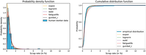
Positive distribution functions from the exponential family are used to describe the remaining data without zeros. Our scrap data shows two different behaviours. The first is an exponential decay right after the zero values. The second describes a right-skewed behaviour with a local extreme value located in the $[1\mathrm{\%},10\mathrm{\%}]$ interval. The modelling of the scrap rates is a counting problem of how much scrap occurred in a set of produced items. In general, this type of data could be described by a discrete model. However, for larger and varying sets, the rate of scrap can also be represented by a continuous distribution. We use this approach which gave our data set better results than discrete approaches like the binomial distribution. Due to the shapes of the scrap data, we used continuous distributions from the exponential family. In particular, the exponential-, log-normal-, fatigue-life- and the wald-distribution were used to find a good approximation model for the data (Thomopoulos, 2018). In addition, an instance of the Gumbel-r distribution (Walck, 1996) was fitted, which turns out to be a bad choice for the data as shown by the goodness of fit evaluation in the model selection process. The distributions were fitted to the data using a maximum likelihood (ML) estimator, which is a common way to fit such distributions to data (Law, 2015). An example of the fitting results can be seen in Figures 5 and 6, where scrap rate data sets for a human controller and automatic control by a machine have been compared. It can be noticed that a human controller results in a scrap with a much lower variance.

Figure 5. Fitted distributions on a sample data set of machine scrap rates.

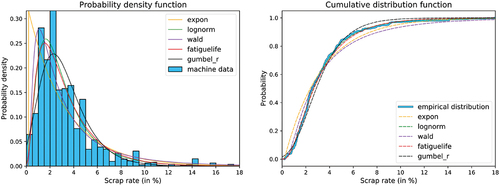
Figure 6. Fitted distributions on a sample data set of human worker scrap rates.

5.2. Processing times

Processing times are the central data in any production process and differ in their structure significantly from scrap data. Most processing time data sets show a normally distributed or slightly right-skewed behaviour. In some cases, the processing times exhibit bi- or multi-modal behaviour, which can also cause the data to split up into different time intervals. This may be correlated with the setup or changeover times of the machine being used.

5.2.1. Outliers

To get rid of the outliers in the processing time data sets, we use a basic one-dimensional clustering algorithm. This approach decides for each data entry if it’s in or near a cluster interval. If this is the case, the entry is assigned to this cluster; if not, it builds a new cluster. An advantage of this outlier detection method is that it probably splits the data into multiple parts for each cluster. Furthermore, clusters can be modelled individually, which leads to a mixture modelling approach for the data set.

5.2.2. Probability distributions

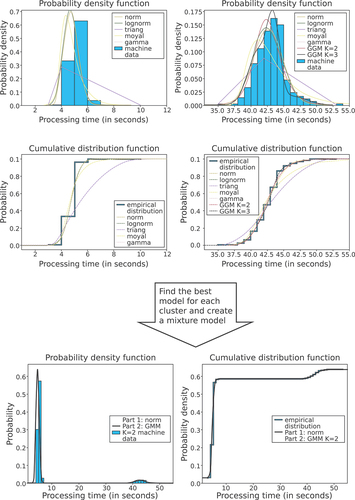
To model the process data, we use distributions that showed good results in similar problem environments (Bongomin et al., 2020). According to this, the normal-, log-normal-, triangular, Moyal-, and gamma-distributions were fitted to our data sets (Evans et al., 2011; Thomopoulos, 2018). These distributions can easily be fitted with an ML estimator, just like for the scrap rate models. Standard distributions are not an adequate solution for the multi-modal data. In these cases, a good approximation can be reached by using Gaussian mixture models (GMM) (Frühwirth-Schnatter et al., 2018). For this purpose, an EM algorithm is used for the parameter estimation (Dempster et al., 1977). One example result of this process is shown in Figure 7. The data sets, which are divided in the preprocessing step into several clusters, are first modelled individually and then assembled into a mixed model. This works by accumulating the distribution functions scaled with the proportion of each cluster to the whole data set as a summation. An example of this procedure is shown in Figure 8. Because of the differences in the processing times and the scrap rates we use a modified version of the procedure presented in Section 5.1 for the processing times. The procedure is extended by a fitting step, in which GMM’s with $\mathcal{K}$ distinct normal distributions are computed and their weights are fitted to the data. This step is only executed when the actual data set contains sufficient information for the successful usage of the EM algorithm. The two-part model step has been slightly modified so that it is only used for mixing the models. It will only be executed assuming the data has been split into several clusters.

Figure 7. Fitted distributions on a sample data set of machine processing times.

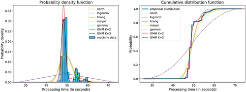
Figure 8. Model fitting process on a sample data set of machine processing times with multiple clusters.

6. Live fitting

The modelling of process data proposed above is usually an offline approach that is part of building a simulation model for the production process. The approach works well if the production system and its environment show homogeneous behaviour over a long time. This is rarely the case in contemporary productions that are much more flexible with changing environmental conditions. This flexibility implies that scrap rates and processing times change and related simulation models, which are used for analysis and optimisation, have to adopt these changes. We propose a streaming approach for this purpose, denoted as live fitting. There are in principle two situations. First, the incoming data shows a homogeneous behaviour. Then additional data can be used to improve the distributions used in the simulation model. This is in particular important for scrap where a larger amount of data helps to find good representations of the data. Second, the observed process changes its behaviour. Then the old models are no longer valid and new distributions have to be estimated. The related problem is the detection of change points.

6.1. Online estimation of distributions

The online estimation of distributions is a one-pass approach where the old data cannot be completely stored. Thus, a streaming approach is required that uses only the most recent data. For live fitting of distributions, two cases have to be distinguished, namely standard distributions like normal, log-normal, Moyal, triangular, or gamma distribution where the ML estimators of the parameters can be derived from specific characteristics of the data like the mean or standard deviation and mixture distribution where an EM-algorithm has to be applied. For standard distributions, parameter estimation is fast if the required quantities like the mean or sample variance of the data are available. For streaming data mean and variance are estimated using the Welford algorithm (Chan et al., 1983). Let ${\bar{x}}_{\mathit{k}-1}$ be the estimated mean and ${\hat{s}}_{\mathit{k}-1}^2$ the estimated variance after $\mathit{k}-1$ observations and let $x_k$ be the next value that arrives, then the new estimates for mean and variance are computed as

${\bar{x}}_{\mathit{k}}={\bar{x}}_{\mathit{k}-1}+\frac{1}{k}\left(x_k-{\bar{x}}_{\mathit{k}-1}\right)\mathrm{and}{\hat{s}}_{\mathit{k}}^2={\hat{s}}_{\mathit{k}-1}^2+\left(x_k-{\bar{x}}_{\mathit{k}-1}\right)\left(x_k-{\bar{x}}_{\mathit{k}}\right)$

Afterwards, only the new estimates have to be stored. The computed variance is not exact but usually, a very good approximation which is sufficient for parameter estimation. From the quantities, the parameters of standard distributions can be estimated. This has not to be done for every new data point. For the first parameter estimation at least $\mathit{k}=30$ data point should be available, the $\mathit{n}$-th new estimation is done after $10\cdot n^{1.9}$ data points. In this way, the number of data points between estimates increases because the estimates become more stable if more data is available. In a new estimation step, the parameters for a set of standard distributions are recomputed. To select the best probability distribution for the available data, a two-sample Kolmogorov-Smirnov-test (Hodges, 1958) (or KS-test for short) is applied to two random samples from the data and the fitted distributions. The best distribution is then selected according to the $\mathit{p}$-values of the KS-test and used for the representation of the data in the simulation model. Thus, the distribution may change in the simulation model, if more data becomes available.

More complex is the online estimation for mixture distributions. In this case, the EM-algorithm has to be used on the new data points which requires more effort. However, online versions of the algorithm are available (Cappé & Moulines, 2009; Kaptein & Ketelaar, 2018) and since new data points usually change the parameters of the distribution only slightly, the algorithm converges usually quickly to a new stationary point when started with the parameters of the distribution that has been fitted according to the past data. The resulting models can then be compared with standard distributions using the two-sample KS-Test. In the case of multimodal data, mixture models, fitted by the EM-algorithm, are usually the best choice. Again the improved distribution is afterwards integrated into the simulation model of the system.

6.2. Change point detection

The methods from the previous subsection improve a fitted distribution, if more data becomes available. However, they rely on the assumption of identically distributed data or data that changes only very slowly its characteristics. In modern production environments, environmental or internal conditions may change quickly resulting in data with significantly different characteristics. If these changes are not detected, simulation models, based on old data, are invalid for analysis and optimisation of the production system.

Change point detection is a method to detect as soon as possible that data changes its characteristics and a new distribution has to be fitted to the data. The problem with change point detection is the distinction between changes that result from stochastic fluctuation and those that result from a change point. Change point detection is based on histograms and time windows. First, a histogram of all data since the last change point is kept. This histogram is updated with every new data sample. Cell width and location can be either chosen based on a priori information or can be computed based on the available data (Scott, 1979). Additionally, a histogram is generated from the data in an observation interval that covers the last $\mathcal{O}$ data points.

A change point is assumed if the two histograms differ. For measuring the difference between the two histograms the Kullback-Leibler divergence (KLD) is used, which has shown to be a good measure for this purpose (Sebastião et al., 2008). A change point is more likely if the KLD increases. Thus, if the maximum of the KLD from the observation changes $\mathit{\kappa }$-times in a row, a change point is assumed, where $\mathit{\kappa }\in [3,5]$ seems to be a good choice. The method is sensitive to the size of the observation window $\mathcal{O}$. If the window is too small, then the method becomes too sensitive. If it is too large, the time until a change point is detected becomes too large. The window size depends on the data, in particular, the variance or better the scale-invariant squared coefficient of variation (SCV) may be used. The size of the window is then $\mathcal{O}=\mathit{\alpha SC}{V}^{\beta }$ for appropriate constants $\mathit{\alpha },\mathit{\beta }>0$. However, $\mathit{\alpha }$ and $\mathit{\beta }$ are very much application and data-dependent and have to be adjusted according to the available data.

If a change point is detected, past data is no longer valid and the whole process of distribution and parameter fitting starts again with the new data after the change point occurred. Thus, if a change point is erroneously detected, the quality of the fitted distribution becomes worse because it results from fewer data points.

7. Evaluation

The application case used for the evaluation is the production of an automotive supplier, which belongs to a supply chain in an international network of factories. The production segments are shown in Figure 1. The two-stage production process for which production will be planned and data is analysed in the evaluation of this paper includes the processes of injection moulding and painting. In the company, a single organisational unit is responsible for the simultaneous planning and control of both segments.

While there are three machines in the first stage, there is only one machine in the second stage. The machines have unrelated processing times per job. At every machine, there is a detection point for scrap to identify it automatically and additionally, at every stage, there is a point to analyse the products manually to reject defective parts. In total, there are four detection points at the first stage and two at the second stage.

To generate the presented results python 3.8.8 was used (Van Rossum & Drake, 2009). To fit distribution models to data, the packages scipy.stats (Virtanen et al., 2020) and scikit-learn (Pedregosa et al., 2011) provided a remedy. The scipy.stats package comes with over 70 implemented distribution functions, which all could be used for (live) fitting the data in our approach.

7.1. Goodness of fit

In the following, we summarise some results for the modelling of production data. We focus on the actual modelling with different probability distributions and assume that the data has already been preprocessed, e.g., outliers have been removed, the steps for handling zero-inflated data have been applied etc. (cf. Section 5).

7.1.1. Scrap

As mentioned in Section 5 we use several distributions from the exponential family (i.e., exponential-, log-normal-, fatigue-life-, wald-distribution, and additionally the Gumbel-r distribution) for modelling scrap rates. To assess the goodness of fit and to pick the best distribution from the ones mentioned above we use the KS-test, i.e., the distribution that yields the highest p-value is considered best. For larger data sets, which may occur in our setting, the KS-test tends to return small p-values, making it difficult to compare the fitted distributions. This is a well-known problem with the KS-test for large data sets and has for example been addressed in Buchholz and Kriege (2014) or Javadi et al. (2013). Instead of applying the test to the complete empirical data set, we draw a smaller random sample of size 30 from the set and perform the test with that sample. This is repeated until the mean of the p-values is stable. Of course, there are further methods to assess the goodness of fit, e.g., graphical measures like PP- or QQ-plots. However, our experiments showed that those measures usually confirm the results of the KS-test.

An example is shown in Figure 9, which contains the QQ- and PP-plots for a fatigue-life- and a Gumbel-r distribution fitted to the same scrap data. For the fatigue-life distribution, the KS-test returned a high p-value and both plots show that the distribution is indeed a good fit for the data. In contrast, the Gumbel-r distribution has a much lower p-value. The poorer goodness of fit is confirmed by the QQ- and PP-plots for that distribution that differ much more from the diagonal line.

Figure 9. Example PP- and QQ-Plots for machine scrap data.

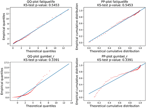
Since, in addition, the KS-test can be performed automatically (in contrast to graphical methods) this approach turned out to be a good choice for selecting the best distribution.

Table 2 shows the results of the KS-test for the fitted distributions and example scrap rate data sets from the machine and human stages. The corresponding plots of probability density and cumulative distribution function can be found in Figures 5 and 6, respectively. In these cases, the best fit is provided by the log-normal distribution followed by the fatigue-life distribution.

Table 2. Evaluation of KS-test for example scrap rate data sets.

	Machine stage	Human stage
	(Figure 5)	(Figure 6)
Distribution	$\mathit{p}-\mathit{value}$	$\mathit{p}-\mathit{value}$
Exponential	0.38458	0.23483
Log-normal	0.58433	0.42257
Wald	0.48264	0.32111
Fatigue-life	0.55839	0.37582
Gumbel-R	0.33428	0.35412

This example is representative of the results of the scrap rate data sets. Table 3 gives an overview of how often a particular distribution was selected as the distribution with the best goodness of fit according to the KS-test for the different stages. As one can see, log-normal- and fatigue-life- distributions are among the most selected distributions in all cases and therefore, provide a good choice for fitting the scrap rates in general. In addition, we listed the number of data sets, that did not contain a sufficient amount of data for fitting.

Table 3. Fitted distributions for scrap rates.

Distribution	Machines Stage 1	Human Stage 1	Machine Stage 2	Human Stage 2
Exponential	2	0	1	1
Log-normal	8	16	31	6
Wald	10	2	9	0
Fatigue-life	10	1	16	0
Gumbel-R	1	0	0	1
Insufficient data	83	20	57	6

7.1.2. Processing times

The fitting procedure for the processing times is similar to the one for scrap rates but uses a different set of distributions.

The results of the KS-test for example data sets of the processing times are shown in Table 4. The corresponding plots of density and distribution can be found in Figures 7 and 8. For these examples, GMM and normal distributions provided the best goodness of fit.

Table 4. Evaluation of KS-test for example processing time data sets.

	Machine stage 1	Machine stage 2	Machine stage 2
	(Figure 7)	part 1 (Figure 8)	part 2 (Figure 8)
Distribution	$\mathit{p}-\mathit{value}$	$\mathit{p}-\mathit{value}$	$\mathit{p}-\mathit{value}$
Normal	0.07036	0.03559	0.3989
Log-normal	0.10744	0.03357	0.4211
Triangular	0.01450	0.00096	0.18197
Moyal	0.10228	0.03243	0.30571
Gamma	0.10803	0.02653	0.39121
GMM $\mathcal{K}=2$	0.32781	-	0.51161
GMM $\mathcal{K}=3$	0.32682	-	0.44708

In general, these two classes of distribution are among the most selected distributions according to the KS-test as one can see from Table 5. However, there is a slight difference between the two stages, as for the second stage triangular distributions are a good choice as well. When analysing the results, it turned out that in cases where the GMM’s were generated, they usually represented the best model. In the other cases one of the other fitted distributions provided a good model instead, which confirms the distribution models used in Bongomin et al. (2020).

Table 5. Fitted Distributions for Processing Times.

Distribution	Machine stage 1	Machine stage 2
Normal	23	18
Log-normal	1	11
Triangular	12	19
Moyal	6	9
Gamma	14	2
GMM $\mathcal{K}=2$	89	16
GMM $\mathcal{K}=3$	21	2
Insufficient data	1	1

7.2. Live fitting

The proposed algorithm for live fitting of production data consists of two main steps that influence the fitting quality: Change point detection and the actual fitting of the data stream starting at the last change point.

At a change point the characteristics of the data stream change, implying that the current distribution is not a good fit anymore. Hence, for undetected change points (i.e., a false negative) the live fitting algorithm would return an outdated distribution. False positives (i.e., the algorithm assumes a change point, but the input data stream has not changed) are less severe because the algorithm keeps at least the current distribution but all other internal data is reinitialised (cf. Section 6).

In contrast to the results from Section 7.1 we do not fit the complete data set here but have to update our distribution(s) for every new value in the data stream.

In the following we present some experimental results for live fitting processing times and scrap rates that focus on the two described main steps of the algorithm.

7.2.1. Processing times

Our real-world data sets do not contain data that allows for a systematic evaluation of the sensitivity of the change point detection. Therefore, we use the following experiment setup: From the real-world data we pick the processing times $\mathbf{x}=x_1,\dots ,x_n$ belonging to one particular machine and article combination. Let $F_x$ be the empirical distribution defined by the $x_i$. Furthermore, let $({\mu }_1,\dots ,{\mu }_l)$ and $({\sigma }_1,\dots ,{\sigma }_m)$ be factors for the variation of mean and standard deviation, respectively. Then, we can define sequences

${\mathbf{y}}_{{\mu }_j}=\mathbf{x}\cdot {\mu }_j$

and

${\mathbf{y}}_{{\mathit{\sigma }}_{\mathbf{k}}}=\left(\mathbf{x}-\stackrel{\mathbf{ˉ}}{\mathbf{x}}\right)\cdot {\sigma }_k+\bar{x}$

where $\bar{x}$ is the mean value of the elements $\mathbf{x}$. The ${\mathbf{y}}_{{\mu }_j}$ have a different mean value than the $\mathbf{x}$, i.e., are shifted to the left or right, while the ${\mathbf{y}}_{{\sigma }_k}$ have the same mean value but a different standard deviation, i.e., are scaled. Let $F_{y_{{\mu }_j}}$ and $F_{y_{{\sigma }_k}}$ be the corresponding empirical distributions.

Finally, we create the input streams for change point detection by sampling $5000$ elements from $F_x$, followed by $1000$ elements from one of the $F_{y_{{\mu }_j}}$ or $F_{y_{{\sigma }_k}}$, followed by $5000$ elements from $F_x$ again, i.e., we use the normal behaviour from the real world data interrupted by an anomaly for the input sequence. Thus, the input stream has change points after $5000$ and $6000$ elements. For each $F_{y_{{\mu }_j}}$ and $F_{y_{{\sigma }_k}}$ we run $100$ replications.

In the following, we present the results for three different machine and job combinations. For simplicity and to anonymise the data we denote the machines with “A, B, C, …” and jobs with “$1,2,3,\dots$”.

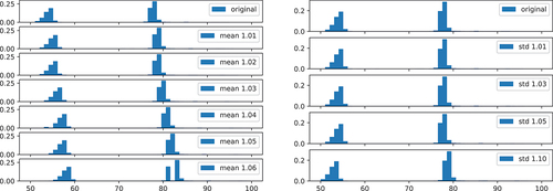
Table 6 shows the results of the change point detection for the first machine and article combination. The change point detection assessed $1100000$ trace elements for each variation factor with a total of $200$ change points (resulting from $100$ replications with $11000$ elements and two change points). The first change point that is detected after there was a change point in the input stream is considered a true positive (TP). All other detected change points are counted as false positives (FP). We have false negatives (FN) if change point detection does not report a change point after it occurred in the stream. The remaining elements in the input stream are considered true negative (TN). Since our definition of TP only requires that the algorithm detects a change point at all, we need another measure for the time consumed until detection. Steps 1 and steps 2 in Table 6 provide the mean number of elements observed in the input stream before the first or second change point was detected.

Table 6. Change point detection for varying mean and variance values of the processing times (machine A, article 1).

type of variation	factor	TP	TN	FP	FN	steps 1	steps 2
mean, ${\mu }_j=$	1.01	1	1099800	0	199	–	362.0
	1.02	200	1099799	1	0	39.81	42.58
	1.03	200	1099800	0	0	24.56	24.56
	1.04	200	1099798	2	0	14.22	17.14
	1.05	200	1099799	1	0	13.23	15.89
	1.06	200	1099799	1	0	11.22	12.18
std, ${\sigma }_k=$	1.01	3	1099800	0	197	57.67	–
	1.03	4	1099800	0	196	233.0	–
	1.05	162	1099798	2	38	89.44	70.89
	1.10	200	1099800	0	0	45.14	49.66

As one can see from the table, the algorithm can already detect the change points for small variations of the mean in this example and yields only a few false positives. Further increasing the factor ${\mu }_j$ for the distributions that define the anomaly in the input stream reduces the number of steps required to detect the change point. If we vary the standard deviation a larger factor is necessary to detect the change point.

Figure 10 shows the histograms of the original values sampled from $F_x$ and the values sampled from the $F_{y_{{\mu }_j}}$ and $F_{y_{{\sigma }_k}}$ to get an impression how much the distribution is shifted or scaled at the change point. This confirms our observation that already small changes are successfully detected.

Figure 10. Histograms of processing times for different change points (Machine A, Article 1).

Table 7 and Figure 11 contain the results from the second machine/article pair. Change point detection was slightly more difficult in this case, resulting in more false positives in general and a larger factor for the variation of the standard deviation required by the algorithm for successful detection. From the number of steps in Table 7 one can also see, that the first change point was easier to detect than the second one.

Figure 11. Histograms of Processing Times for different Change Points (Machine B, Article 2).

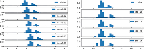
Table 7. Change point detection for varying mean and variance values of the processing times (Machine B, Article 2).

type of variation	factor	TP	TN	FP	FN	steps 1	steps 2
mean, ${\mu }_j=$	1.01	98	1099783	17	102	55.81	529.69
	1.02	198	1099765	35	2	40.13	46.43
	1.03	200	1099772	28	0	27.08	25.7
	1.04	200	1099769	31	0	21.92	20.94
	1.05	200	1099770	30	0	19.26	16.86
	1.06	199	1099761	39	1	19.04	14.49
std, ${\sigma }_k=$	1.20	115	1099779	21	85	87.3	185.41
	1.24	148	1099771	29	52	91.15	191.57
	1.30	155	1099777	23	45	74.4	156.96
	1.36	195	1099773	27	5	43.62	56.80

The results for the third machine/article pair shown in Table 8 and Figure 12 support our observations from the previous experiments.

Figure 12. Histograms of Processing Times for different Change Points (Machine C, Article 3).

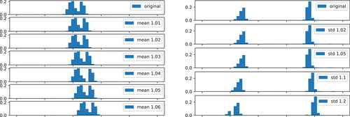
Table 8. Change point detection for varying mean and variance values of the processing times (Machine C, Article 3).

type of variation	factor	TP	TN	FP	FN	steps 1	steps 2
mean, ${\mu }_j=$	1.01	107	1099781	19	93	131.78	121.18
	1.02	190	1099776	24	10	42.28	68.49
	1.03	195	1099777	23	5	32.65	35.94
	1.04	200	1099767	33	0	19.92	22.23
	1.05	200	1099777	23	0	16.78	18.74
	1.06	200	1099770	30	0	15.66	16.7
std, ${\sigma }_k=$	1.02	2	1099800	0	198	71.0	–
	1.05	168	1099800	0	32	84.29	70.85
	1.1	200	1099798	2	0	46.19	47.67
	1.2	200	1099800	0	0	20.64	15.8

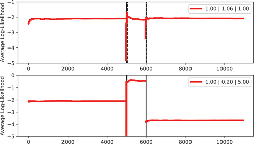
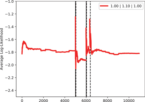
Figure 13 shows the evolution of the average log-likelihood of a normal distribution fitted to input streams resulting from two different setups of change points. The first input trace is from one of the replications summarised in Table 7, i.e., the input sequence consists of original data (factor $1.0$) and data with a mean value varied by factor $1.06$. As one can see the average log-likelihood converges very fast, implying that the live-fitting approach has converged as well. The real change points are marked with a solid vertical line in the figure, while the detected change points are marked with a dashed line. In this case, the change points have been detected only a few steps after they occurred, such that the lines almost overlap. Because of the reset of the algorithm, the log-likelihood declines for a short period, but the algorithm can find a suitable new distribution after a couple of new trace elements have been observed. For the second plot in Figure 13 we changed the input trace by modifying the mean by factors $0.2$ and $5.0$, respectively. Of course, these change points are much easier to detect for the algorithm, but it is also more important that the algorithm provides a new distribution in time, because of the larger changes in the input stream.

Figure 13. Average log-likelihood for processing times (Machine B, Article 2).

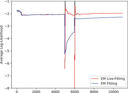
For the previous examples, we used standard distributions that can be fitted using some derived measures from the input stream. As we have seen in Section 7.1.2 GMMs are often the best choice for processing times. Moreover, the distributions from Figure 10 with two peaks look like a candidate for a GMM $\mathcal{K}=2$. GMMs have to be fitted using an EM algorithm and Figure 14 shows a comparison of our EM live fitting and an offline EM approach. The live fitting approach uses one EM iteration for each new observation to update its distribution. The offline approach gets the complete sequence observed so far as input and may iterate until convergence. For the original data the two algorithms behave almost identically, but at change points the live fitting approach recovers much faster because the offline approach lacks the change point detection and still considers the old deprecated values.

Figure 14. Comparison of average log-likelihood for processing times (Machine A, Article 1) using the EM algorithm for GMMs.

7.2.2. Scrap

For the scrap rates, we conducted similar experiments as described for the processing times above.

Tables 9 and 10 show the summary of the change point detection for systematic variation of mean and standard deviation values. The corresponding distributions are shown in Figures 15 and 16. In general, the change points for the scrap rates were more difficult to detect than the ones for the processing times, since the distributions have a larger variance.

Figure 15. Histograms of scrap rates for different change points (Machine D, Article 4).

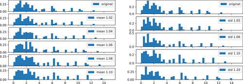
Figure 16. Histograms of scrap rates for different change points (Machine E, Article 5).

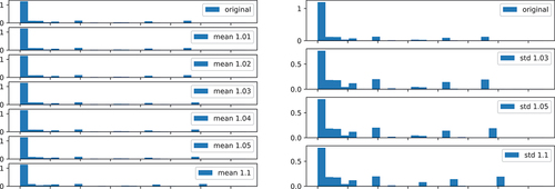
Table 9. Change point detection for varying mean and variance values of the scrap rates (Machine D, Article 4).

type of variation	factor	TP	TN	FP	FN	steps 1	steps 2
mean, ${\mu }_j=$	1.02	72	1099767	33	128	99.67	1028.05
	1.04	167	1099755	45	33	44.45	69.58
	1.06	192	1099755	45	8	32.70	40.59
	1.08	197	1099744	56	3	29.6	78.79
	1.10	196	1099743	57	4	27.64	40.57
std, ${\sigma }_k=$	1.02	38	1099766	34	162	139.00	2137.60
	1.06	52	1099772	28	148	111.06	410.94
	1.1	152	1099749	51	48	43.75	250.80
	1.2	187	1099748	52	13	31.19	160.30

Table 10. Change point detection for varying mean and variance values of the scrap rates (Machine E, Article 5).

type of variation	factor	TP	TN	FP	FN	steps 1	steps 2
mean, ${\mu }_j=$	1.01	6	1099796	4	194	158.0	3366.4
	1.02	4	1099792	8	196	-	2698.25
	1.03	28	1099794	6	172	144.08	1730.8
	1.04	137	1099791	9	63	55.15	209.34
	1.05	144	1099784	16	56	58.87	138.02
	1.1	193	1099786	14	7	32.93	45.58
std, ${\sigma }_k=$	1.03	9	1099791	9	191	270.5	2935.0
	1.05	147	1099790	10	53	72.83	242.17
	1.1	199	1099784	16	1	34.8	92.22

Figure 17 shows the evolution of the likelihood of a log-normal distribution when fitting one of the examples from Table 9. One can see, that change point detection has a false positive here, but it is also visible that the algorithm recovers fast from this.

Figure 17. Average log-likelihood for scrap rates (Machine D, Article 4).

7.3. Optimization

To show the effect of updated deterministic processing times in the schedule, a scenario with 13 jobs was selected and 4 machines in two production stages (see Figure 1) are included in the production scenario. In this scenario, jobs in the second stage can only be started after they have been completed in the first stage (see exemplary job 2 in Figure 18). To optimise the machine schedules, the algorithms Shortest Processing Time First (SPT) and Local Search are used following Schumacher and Buchholz (2020) and their SPT combined with Random Descent (shift). SPT sorts the jobs according to their process times in ascending order and thus schedules them one by one on the machines and the different stages. Random Descent (shift) places one randomly selected job to another position in the existing schedule and accepts the resulting solution if it has a better makespan. The optimisations were conducted on an Intel®Core^TMi7–3770 CPU with 24 GB RAM on Windows 10 Pro running Java 1.8. All calculations finished in less than one second each.

Figure 18. Modified schedule due to change point detection.

Exemplary, the processing times for producing one part of job 2 are increased with the factor 1.04 (see Section 7.2.1). Instead of having a duration of 39.4 hours in the upper schedule of Figure 18, after adjustment job 2 has a duration of 40.8 hours. The makespan $C_{\mathit{max}}$ is also extended from 59.4 hours to 60.3 hours. The makespan defines the time between the beginning of the first and the end of the last job, which is to be planned. These effects would be similar in the case of an increased scrap rate. In this case, the number of jobs would be adjusted and jobs would extend in duration as well (see Section 4). The lower schedule in this example has a higher makespan and the schedule has been rearranged due to the changes in the lengths of job 2 as well as the stochastic influences in the local search algorithm. Thus, the makespan does not lengthen as much as the job duration increases. For more optimisation examples using the data architecture of Figure 2 in a use case with real data from the automotive industry, see Schumacher (2023).

8. Results and outlook

In this paper, we model probability distributions and estimate their parameters from real-world data sets of processing times and scrap rates. The fitting approaches, which were applied to data from a real production system, compare the goodness of fit for different distributions. Results show that in stage 1 the processing times are best modelled by a normal distribution or a GMM. For processing times of machines in stage 2, additionally, the triangular distribution yields good results. The scrap rates for the human stages followed in most cases a log-normal distribution, while for the machine stages the picture was not that clear as the best distribution was either log-normal, wald, or fatigue-life. The quality of the results for live fitting heavily depends on the change point detection and our experiments showed that the approach can reliably react to even small changes in the input data. Using the developed techniques data, probability distributions, and their estimations are categorised and a concept is developed to use it for optimising scheduling problems with methods combining simulation and optimisation models. Calculating optimal schedules is important for production systems to reduce makespan and assure timely production. It can be seen that heuristic algorithms in scheduling may partially compensate for an increase of input parameters as long as it has been identified.

The vision of the research presented in this paper is an online approach that efficiently computes quasi-optimal schedules for production systems based on current data from the system and its environment. In the future we want to further integrate methods to estimate distributions from streaming data, make use of the distributions in simulation models for an online analysis, and combine these results with optimisation algorithms. The integration of live-fitting into simulation models will then extend the available simheuristics framework to an online approach. With the proposed approach, good schedules can be provided, even if the production scenario changes.

Disclosure statement

No potential conflict of interest was reported by the author(s).

References

- Aminikhanghahi, S., & Cook, D. J. (2017). A survey of methods for time series change point detection. Knowledge and Information Systems, 510(2), 339–367. https://doi.org/10.1007/s10115-016-0987-z
- Balci, O. (2003). Verification, validation, and certification of modeling and simulation applications. Proceedings of the 2003 Winter Simulation Conference, New Orleans, LA, USA (Vol. 1, pp. 150–158).
- Bauernhansl, T., ten Hompel, M., and Vogel-Heuser, B. editors. (2014). Industrie 4.0 in Produktion, Automatisierung und Logistik – Anwendung, Technologien, Migration. Springer Vieweg. ISBN 3658046821.
- Bongomin, O., Mwasiagi, J., Oyondi Nganyi, E., & Ildephonse, N. (2020). A complex garment assembly line balancing using simulation-based optimization. Engineering Reports, 2(11), 1–23. https://doi.org/10.1002/eng2.12258
- Buchholz, P., Dohndorf, I., & Kriege, J. (2019). An online approach to estimate parameters of phase-type distributions. In 2019 49th Annual IEEE/IFIP International Conference on Dependable Systems and Networks (DSN), Portland, Oregon, USA (pp. 100–111). IEEE.
- Buchholz, P., & Kriege, J. (2014). Markov modeling of availability and unavailability data. In Proceedings of the 2014 Tenth European Dependable Computing Conference, EDCC ‘14 (pp. 94–105). IEEE Computer Society. USA. https://doi.org/10.1109/EDCC.2014.22 ISBN 9781479938049.
- Cappé, O. (2011). Online expectation-maximisation. Mixtures: Estimation and Applications, 1, 31–53. https://doi.org/10.1002/9781119995678.ch2.
- Cappé, O., & Moulines, E. (2009). On-line expectation–maximization algorithm for latent data models. Journal of the Royal Statistical Society: Series B (Statistical Methodology), 710(3), 593–613. https://doi.org/10.1111/j.1467-9868.2009.00698.x
- Chan, T. F., Golub, G. H., & LeVeque, R. J. (1983). Algorithms for computing the sample variance: Analysis and recommendations. American Statistician, 370(3), 242–247. https://doi.org/10.1080/00031305.1983.10483115
- Chandola, V., & Kumar, V. (2009). Outlier detection: A survey. ACM Computing Surveys, 41(3), 1–58. https://doi.org/10.1145/1541880.1541882
- Clausen, U., Diekmann, D., Pöting, M., & Schumacher, C. (2017). Operating parcel transshipment terminals – a combined simulation and optimization approach. Journal of Simulation, 110(1), 2–10. https://doi.org/10.1057/s41273-016-0032-y ISSN 1747-7778.
- Dastjerdy, B., Saeidi, A., & Heidarzadeh, S. (2023). Review of applicable outlier detection methods to treat geomechanical data. Geotechnics, 30(2), 375–396. https://doi.org/10.3390/geotechnics3020022 ISSN 2673-7094.
- Dempster, A. P., Laird, N. M., & Rubin, D. B. (1977). Maximum likelihood from incomplete data via the EM algorithm. Journal of the Royal Statistical Society: Series B (Methodological), 390(1), 1–22. https://doi.org/10.1111/j.2517-6161.1977.tb01600.x
- Duan, N., Manning, W. G., Morris, C. N., & Newhouse, J. P. (1983). A comparison of alternative models for the demand for medical care. Journal of Business & Economic Statistics, 10(2), 115–126. https://doi.org/10.1080/07350015.1983.10509330
- Evans, M., Hastings, N., Peacock, B., & Forbes, C. (2011). Statistical distributions. Wiley. ISBN 9781118097823.
- Fan, K., Zhai, Y., Li, X., & Wang, M. (2018). Review and classification of hybrid shop scheduling. Production Engineering, 120(5), 597–609. https://doi.org/10.1007/s11740-018-0832-1 ISSN 0944-6524.
- Figueira, G., & Almada-Lobo, B. (2014). Hybrid simulation–optimization methods – a taxonomy and discussion. Simulation Modelling Practice and Theory, 46, 118–134. https://doi.org/10.1016/j.simpat.2014.03.007 ISSN 1569190X.
- Fowler, J. W., & Rose, O. (2004). Grand challenges in modeling and simulation of complex manufacturing systems. Simulation, 800(9), 469–476. https://doi.org/10.1177/0037549704044324
- Frühwirth-Schnatter, S., Celeux, G., & Robert, C. (2018). Handbook of mixture analysis. CRC Press.
- Gendreau, M., & Potvin, J.-Y. (2019. Handbook of metaheuristics, volume 272 of International series in operations research & management science (3rd ed.). Springer International Publishing. https://doi.org/10.1007/978-3-319-91086-4 ISBN 978-3-319-91085-7
- Gholami, M., Zandieh, M., & Alem-Tabriz, A. (2009). Scheduling hybrid flow shop with sequence-dependent setup times and machines with random breakdowns. International Journal of Advanced Manufacturing Technology, 420(1–2), 189–201. https://doi.org/10.1007/s00170-008-1577-3. PII: 1577.
- Goodall, P., Sharpe, R., & West, A. (2019). A data-driven simulation to support remanufacturing operations. Computers in Industry, 105, 48–60. https://doi.org/10.1016/j.compind.2018.11.001
- Hodges, J. L. (1958). The significance probability of the Smirnov two-sample test. Arkiv för matematik, 30(5), 469–486. https://doi.org/10.1007/BF02589501
- Javadi, B., Kondo, D., Iosup, A., & Epema, D. (2013). The failure trace archive: Enabling the comparison of failure measurements and models of distributed systems. Journal of Parallel and Distributed Computing, 730(8), 1208–1223. https://doi.org/10.1016/j.jpdc.2013.04.002 ISSN 0743-7315.
- Juan, A. A., Faulin, J., Grasman, S. E., Rabe, M., & Figueira, G. (2015). A review of simheuristics – extending metaheuristics to deal with stochastic combinatorial optimization problems. Operations Research Perspectives, 2, 62–72. https://doi.org/10.1016/j.orp.2015.03.001 ISSN 22147160.
- Kaptein, M., & Ketelaar, P. (2018). Maximum likelihood estimation of a finite mixture of logistic regression models in a continuous data stream. arXiv preprint arXiv:1802.10529.
- Kastens, U., & Büning, H. K. (2014). Modellierung: Grundlagen und formale Methoden (3 ed.). Hanser. ISBN 3446442499.
- Laroque, C., Leißau, M., Copado, P., Schumacher, C., Panadero, J., & Juan, A. A. (2022). A biased-randomized discrete-event algorithm for the hybrid flow shop problem with time dependencies and priority constraints. Algorithms, 150(2), 54. https://doi.org/10.3390/a15020054 PII: a15020054.
- Law, A. M. (2011). How the expertfit® distribution-fitting software can make your simulation models more valid. Proceedings of the 2011 Winter Simulation Conference (WSC), Phoenix, Arizona, USA (pp. 63–69). IEEE.
- Law, A. M. (2015). Simulation modeling and analysis (Vol. 5). Mcgraw-hill New York.
- MacCarthy, B. L., & Liu, J. (1993). Addressing the gap in scheduling research – a review of optimization and heuristic methods in production scheduling. International Journal of Production Research, 310(1), 59–79. https://doi.org/10.1080/00207549308956713 ISSN 0020-7543.
- Mandhare, H. C., & Idate, S. R. (2017). A comparative study of cluster based outlier detection, distance based outlier detection and density based outlier detection techniques. In 2017 International Conference on Intelligent Computing and Control Systems (ICICCS) (pp. 931–935). https://doi.org/10.1109/ICCONS.2017.8250601
- Min, Y., & Agresti, A. (2002). Modeling nonnegative data with clumping at zero: A survey. Journal of the Iranian Statistical Society, 10(1), 7–33.
- Morais, M. D. F., Filho, M. G., & Perassoli Boiko, T. J. (2013). Hybrid flow shop scheduling problems involving setup considerations: A literature review and analysis. International Journal of Industrial Engineering, 200(11–12), 614–630. ISSN 10724761.
- Müller, D., Schumacher, C., & Zeidler, F. (2018). Intelligent adaption process in cyber-physical production systems. In T. Margaria & B. Steffen (Eds.), Leveraging applications of formal methods, verification and validation – proceedings of the ISoLA 2018, part III, number 11246 in lecture notes in computer science (pp. 411–428). Springer International Publishing. ISBN 978-3-030-03423-8.
- Nahleh, Y. A., Kumar, A., & Daver, F. (2013). Predicting relief materials’ demand for emergency logistics planning using arena input analyzer. International Journal of Engineering Science and Innovative Technology (IJESIT), 20(5), 318–327.
- Neufeld, J. S., Schulz, S., & Buscher, U. (2023). A systematic review of multi-objective hybrid flow shop scheduling. European Journal of Operational Research, 3090(1), 1–23. https://doi.org/10.1016/j.ejor.2022.08.009 ISSN 0377-2217.
- Pedregosa, F., Varoquaux, G., Gramfort, A., Michel, V., Thirion, B., Grisel, O., Blondel, M., Prettenhofer, P., Weiss, R., Dubourg, V., and Vanderplas, J. (2011). Scikit-learn: Machine learning in Python. Journal of Machine Learning Research, 12(85), 2825–2830. https://doi.org/10.48550/arXiv.1201.0490
- Pinedo, M. (2016). Scheduling – theory, algorithms, and systems (5 ed.). Springer. https://doi.org/10.1007/978-3-319-26580-3 ISBN 9783319265780
- Prajapat, N., & Tiwari, A. (2017). A review of assembly optimisation applications using discrete event simulation. International Journal of Computer Integrated Manufacturing, 300(2–3), 215–228. https://doi.org/10.1080/0951192X.2016.1145812 ISSN 0951-192X.
- Ribas, I., Leisten, R., & Framiñan, J. M. (2010). Review and classification of hybrid flow shop scheduling problems from a production system and a solutions procedure perspective. Computers & Operations Research, 370(8), 1439–1454. https://doi.org/10.1016/j.cor.2009.11.001. ISSN 03050548. PII: S0305054809002883.
- Rousseeuw, P. J., & Hubert, M. (2011). Robust statistics for outlier detection. WIREs Data Mining and Knowledge Discovery, 10(1), 73–79. https://doi.org/10.1002/widm.2
- Ruiz, R. (2018). Scheduling heuristics. In R. Martí, P. M. Pardalos, & M. G. C. Resende (Eds.), Handbook of heuristics (pp. 1197–1229). Springer International Publishing. ISBN 978-3-319-07123-7.
- Ruiz, R., Șerifoǧlu, F. S., & Urlings, T. (2008). Modeling realistic hybrid flexible flowshop scheduling problems. Computers & Operations Research, 350(4), 1151–1175. https://doi.org/10.1016/j.cor.2006.07.014. ISSN 03050548. PII: S0305054806001560.
- Ruiz, R., & Vázquez-Rodríguez, J. A. (2010). The hybrid flow shop scheduling problem. European Journal of Operational Research, 2050(1), 1–18. https://doi.org/10.1016/j.ejor.2009.09.024. ISSN 0377-2217. PII: S0377221709006390.
- Schumacher, C. (2023). Anpassungsfähige Maschinenbelegungsplanung eines praxisorientierten hybriden Flow Shops (1st ed.). Springer Fachmedien Wiesbaden and Imprint Springer Vieweg. https://doi.org/10.1007/978-3-658-41170-1 ISBN 9783658411701
- Schumacher, C., & Buchholz, P. (2020). Scheduling algorithms for a hybrid flow shop under uncertainty. Algorithms, 130(11), 277. https://doi.org/10.3390/a13110277 PII: a13110277.
- Schumacher, C., Buchholz, P., Fiedler, K., & Gorecki, N. (2020). Local search and tabu search algorithms for machine scheduling of a hybrid flow shop under uncertainty. In K.-H. Bae, B. Feng, S. Kim, S. Lazarova-Molnar, Z. Zheng, T. Roeder, & R. Thiesing (Eds.), Proceedings of the 2020 Winter Simulation Conference, Orlando, Florida, USA (pp. 1456–1467).
- Scott, D. W. (1979). On optimal and data-based histograms. Biometrika, 660(3), 605–610. https://doi.org/10.1093/biomet/66.3.605
- Sebastião, R., Gama, J., Rodrigues, P. P., & Bernardes, J. (2008). Knowledge Discovery from Sensor Data. In M. M. Gaber, R. R. Vatsavai, O. A. Omitaomu, J. Gama, N. V. Chawla, & A. R. Ganguly (Eds.), Second International Workshop, Sensor-KDD 2008, Las Vegas, NV, USA, August 24–27, 2008.
- Shapiro, R., White, S., & Bock, C. (2011). BPMN 2.0 handbook second edition: methods, concepts, case studies and standards in business process management notation. Future Strategies. ISBN 9780984976409.
- Shekhar Jha, H., Mustafa Ud Din Sheikh, H., & Lee, W. J. (2021). Outlier detection techniques help us identify and remove outliers in production data to improve production forecasting. SPE/AAPG/SEG Asia Pacific Unconventional Resources Technology Conference, volume Day 1 Tue (pp. 11). November 16, 2021. https://doi.org/10.15530/AP-URTEC-2021-208384. D012S001R040.
- Shimizu, Y. (2022). Multiple desirable methods in outlier detection of univariate data with R source codes. Frontiers in Psychology, 12. https://doi.org/10.3389/fpsyg.2021.819854 ISSN 1664-1078.
- Sobhiyeh, S., & Naraghi-Pour, M. (2020). Online detection and parameter estimation with correlated observations. IEEE Systems Journal, 150(1), 180–191. https://doi.org/10.1109/JSYST.2020.2977926
- Taillard, E. (1993). Benchmarks for basic scheduling problems. European Journal of Operational Research, 640(2), 278–285. https://doi.org/10.1016/0377-2217(93)90182-M. ISSN 0377-2217. PII: 037722179390182M.
- Taillard, E. (2016). Éric taillard’s page. http://mistic.heig-vd.ch/taillard/problemes.dir/ordonnancement.dir/ordonnancement.html
- Thomopoulos, N. T. (2018). Probability distributions (1 ed.). Springer.
- van den Burg, G. J., & Williams, C. K. 2020. An evaluation of change point detection algorithms. arXiv preprint arXiv:2003.06222, 2020.
- Van Rossum, G., & Drake, F. L. (2009). Python 3 reference manual. CreateSpace Independent Publishing Platform. ISBN 1441412697.
- Virtanen, P., Gommers, R., Oliphant, T. E., Haberland, M., Reddy, T., Cournapeau, D., Burovski, E., Peterson, P., Weckesser, W., Bright, J., van der Walt, S. J., Brett, M., Wilson, J., Millman, K. J., Mayorov, N., Nelson, A. R. J., Jones, E., Kern, R. … Halchenko, Y. O. (2020). SciPy 1.0: Fundamental algorithms for scientific computing in python. Nature Methods, 17(3), 261–272. https://doi.org/10.1038/s41592-019-0686-2
- Walck, C. (1996). Hand-book on statistical distributions for experimentalists. Stockholms universitet. Internal Report SUF-PFY/96–01.
- Wang, J., Chang, Q., Xiao, G., Wang, N., & Li, S. (2011). Data driven production modeling and simulation of complex automobile general assembly plant. Computers in Industry, 620(7), 765–775. https://doi.org/10.1016/j.compind.2011.05.004
- Waniczek, M., Niedermayr, R., & Graumann, M. (2017 November). Need for speed – controlling muss schneller werden. Controlling & Management Review, 610(8), 50–56. https://doi.org/10.1007/s12176-017-0100-9
- Warth, J., Kaiser, G., & Kügler, M. (2011). The impact of data quality and analytical capabilities on planning performance: Insights from the automotive industry. 10 Internationale Tagung Wirtschaftsinformatik, Zurich, (pp. 322–331).
- Zuur, A. F., Ieno, E. N., Walker, N. J., Saveliev, A. A., & Smith, G. M. (2009). Zero-truncated and zero-inflated models for count data ( pp. 261–293). Springer. https://doi.org/10.1007/978-0-387-87458-6_11 ISBN 978-0-387-87458-6