The effects of joints on the moisture behaviour of rain exposed wood: a numerical study with experimental validation

ABSTRACT

Joints in timber structures are particularly vulnerable to degradation due to their tendency to trap moisture. The mechanisms involved, and their effect on the moisture conditions of wood, are here investigated numerically. The horizontal member of a rail and post-type configuration is modelled numerically by a two-dimensional diffusion model with material properties for Norway spruce. Contact areas are assumed to be fully wetted when the specimen is exposed to free water but are unable to interact with the ambient air. Water that is absorbed through such areas cannot dry out through the same surface and is instead redistributed. The model was validated against experimental data, both previously unpublished data and data obtained from the literature, including both laboratory and outdoor exposure. The numerical solutions were, in general, consistent with the measured data. The model provides a simple, yet accurate, method to estimate the moisture conditions in certain types of wood joints. In addition, the spatial distribution of time spent above 25% moisture content was calculated, in order to investigate the suitability of the model for durability applications.

KEYWORDS:

• Wood
• moisture transport
• numerical
• joint
• water

1. Introduction

Wood that is exposed outdoors above ground is constantly subjected to cycles of wetting and drying. Understanding how wood responds to wetting is imperative for dealing with deteriorating mechanisms such as cracks or fungal decay, as moisture content is one of the fundamental variables for calculating moisture induced stresses (Angst and Malo 2010) and decay rates (Brischke et al. 2006; Brischke and Thelandersson 2014). Moisture traps are particularly vulnerable to fungal decay due to their tendency to trap and hold moisture over extended time periods, thus facilitating favourable growth conditions.

The rate of water absorption during wetting depends on the intrinsic moisture properties of the material and in which structural direction the water uptake occurs. For example, end-grain surfaces and permeable species such as pine sapwood absorb moisture more rapidly than side-grain or less permeable species such as spruce. Drying depends also on the relative humidity at the wood surface, which in turn depends on the ambient relative humidity and the air flow across the surface. Joints are often subject to elevated moisture contents due to the connecting member obstructing the flow of air over the interface surface area while simultaneously allowing wetting of the same area.

It is well-known that these elevated moisture contents facilitate decay growth, as damages on existing structures are predominantly found in such areas (see Robbers et al. 2018). Also, standardized specimens used for accelerated decay testing in above-ground conditions are, in general, designed as joints to facilitate decay growth (Groot 1992; Meyer et al. 2016). Several research studies have investigated the moisture conditions in joints through continuous moisture monitoring (see Gaby and Duff 1978; Isaksson and Thelandersson 2013; Fredriksson et al. 2016; Niklewski et al. 2018). Yet, as the mechanisms involved are not fully understood, it is challenging to generalize such experimental results. Current methods for considering the effect of joints on the moisture conditions of wood are based on purely empirical models (see Isaksson and Thelandersson 2013; Niklewski et al. 2018). Empirical models rely on long-term measurements for rating the moisture performance of specific joints, which is problematic due to the resource-intensive nature of such measurements. In addition, common techniques employed for continuous moisture monitoring (e.g. resistance-type or gravimetric) have limited ability to map the distribution of moisture in the wood. As discussed by Brischke et al. (2017), using such data as input for durability models can be problematic, since the measurements do not necessarily represent the conditions where decay develops.

Moisture transport can be described with the moisture gradient as the driving potential, a diffusion coefficient that governs the rate of transport in the material and a mass transfer coefficient that governs the interaction with the air. This type of model has predominantly been used for modelling moisture transfer in the hygroscopic moisture range but has also been used to model free water flux (see Derbyshire and Robson 1999; De Meijer and Militz 2000; Virta et al. 2006; Niklewski et al. 2016). Liquid moisture transport is driven by capillary pressure differentials ; however, it is frequently described by the moisture gradient as the driving potential by utilizing the relationship between capillary pressure and degree of saturation (Spolek and Plumb 1981). The transport coefficient can then be described as a function of the intrinsic permeability of the material (see Virta et al. 2006). Alternatively, the transport coefficient can be calculated from the moisture gradients under non-steady state conditions (Koponen 1984; Kang et al. 2009). It should be emphasized that it is difficult to obtain congruent data on moisture diffusion coefficients from the literature, with large variations depending on the measuring technique which is employed (Kumaran 1999). In addition, the rate of moisture transport depends on factors relating to the boundary conditions. For example, the rate of transport during wetting of dry wood is different from the drying of green lumber, due to the higher degree of pit aspiration (Comstock and Côté 1968) and effects related to air-trapping (Virta et al. 2006).

The aim of the present study was to develop a numerical model for moisture-based durability assessment of wooden joints. Previous durability rating of joints (see e.g. Isaksson and Thelandersson 2013; Niklewski et al. 2018) have been based on single-point continuous moisture content measurements. As opposed to conventional moisture monitoring techniques, a numerical analysis gives the entire moisture distribution of the joint in question. As such, numerical modelling can be used in order to determine where a specific joint is most susceptible to decay growth. In addition, it can be used to study the effect of different climates on the moisture conditions and to estimate moisture distributions over time. Ultimately, such a model should be implemented in a durability design framework, following the methodology described by Meyer-Veltrup et al. (2018).

In the present study, the moisture distribution in a specific type of joint was studied through the use of a numerical model based on Fick's second law of diffusion. The study builds on a previous publication (Niklewski et al. 2016), where a one-dimensional model for transverse moisture transport in panels was proposed. In the present study, the focus was instead on the moisture behaviour of joints. Joints are challenging to describe numerically because moisture transport occurs in several directions and the moisture conditions on the boundaries are less well-defined. In order to deal with this problem, the numerical model was extended to two-dimensional moisture transport and the effects of joints were considered by assigning a simple zero-flux boundary condition to interface areas during drying, while simultaneously allowing absorption during wetting. The model performance was evaluated by comparison with laboratory measurements and measurements taken outdoors.

2. Materials and methods

2.1. Laboratory experiment

The experimental setup used in the laboratory experiment is described in detail by Fredriksson et al. (2016). In short, the set-up included three different types of joints, whereof only one was used in the present study. A conceptual illustration of this joint and the relevant points of measurement are shown in Figure 1. The joint consisted of a vertical board ($22\times 90{\mathrm{m}\mathrm{m}}^2$) butted to the side-grain of a horizontal board ($22\times 90{\mathrm{m}\mathrm{m}}^2$). The moisture content sensors were protected from wetting by a box made of acrylic glass (PMMA) which was mounted on the back-side of the boards. The same PMMA box also ensured that only the front side of the joint was directly exposed to spray during the experiment.

Figure 1. Experimental set-up. Each filled circle shows the location of an electrode pair. Units in (mm).

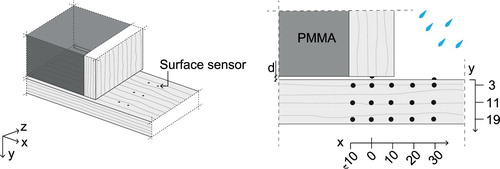
The data set includes measurements on three different gap-sizes (0, 2 and 5 mm) as well as two different types of Norway spruce (Picea abies (L.) Karst); fast-grown and slow-grown with different growth ring width (1–2 mm or 3–9 mm) but similar density (350–400 kg m⁻³). Consequently, six subsets of measurements were available. The measurements showed that the largest gap-size (5 mm) effectively rendered the horizontal board free to dry (Fredriksson et al. 2016). Therefore, as the objective of the present study was to study the effect of moisture trapping, only the two types of specimens having smaller gap-sizes were analysed. In addition, as the model is not suitable for modelling moisture transport in end-grain, the present analysis was limited to the horizontal board.

Resistance-type wood moisture content sensors were mounted in the spatial coordinates given in Figure 1. The duration of surface moisture and water in the gap between the two boards were monitored using sensors described by Fredriksson et al. (2013). The joints were then exposed to two different water spraying sequences:

1. one long period of wetting of 6.5 h (data from Fredriksson et al. 2016);

2. cyclic wetting with a one-hour wetting period each day for 5 consecutive days (data not previously published).

In both cases, the final spray sequence was followed by 300 h of drying at 65% relative humidity (φ) and a constant temperature (T) of 20${}^{\circ }$C. This was also the climate in the room during the wetting periods, but φ increased temporarily during the water spraying. Moisture content, duration of surface moisture and presence of water in the gaps were measured every 5th minute while φ and T in the room were logged continuously. The wind velocity was approximately 0.1–0.2 m s⁻¹, measured on the upper surface of the horizontal member. All specimens had been conditioned to the absorption isotherm at $\phi =$ 65% and $T={20}^{\circ }$C prior to the first spray sequence of 6.5 h.

2.2. Outdoor experiment

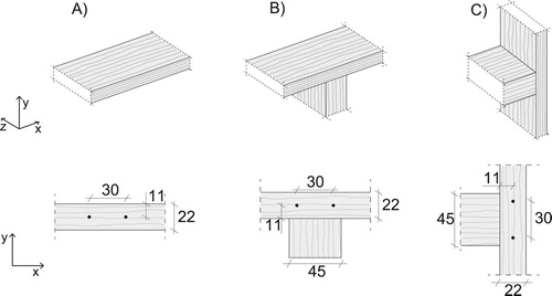
The experimental data on outdoor exposure were obtained from Isaksson and Thelandersson (2013) where the performance of various joints was evaluated by monitoring their moisture content over time while exposed to outdoor climate. The experiment was conducted on a roof (elevation about 10 m) of a building in Lund, Sweden. Each specimen (two replicates) consisted of a Norway spruce board of dimensions $22\times 95{\mathrm{m}\mathrm{m}}^2$ with a secondary member attached. The material was free from defects and had approximately equal growth ring width ; however, wood density and sapwood-content were not documented. Different variations of the connection between the two members were tested, primarily with respect to the size and the orientation of their connecting interface.

The moisture content in the board was measured every hour by use of commercial resistance-type moisture sensors with electrodes located at mid-thickness. No calibration of the measurement system was carried out, meaning that there exists a potential systematic error in the moisture content measurements. However, the general trends regarding the change in moisture content were assumed to depict the actual behaviour. The moisture content was calculated from the resistance by using a function developed by Hjort (1996), which is valid up to approximately 25% moisture content. Any values exceeding 25% were interpreted simply as 25% or higher.

The two joints and the horizontal board shown in Figure 2 were selected for analysis, since they have similar geometry as the one used in the laboratory experiment (see Section 2.1). The moisture content was measured in a single point between two electrodes. The measured output was regarded as being representative for the moisture content at the position of the electrode, as electrodes tend to measure the resistance locally at the wood-electrode interface (Skaar 1964; Norberg 1999; Zelinka et al. 2015).

Figure 2. View of the three specimen types (denoted A–C). Each filled circle represents the location of a single electrode.

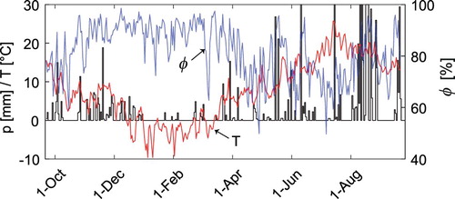
Weather data was recorded on-site. Hourly average values φ and T as well as hourly accumulated precipitation are shown in Figure 3. The average wind velocity was 2 m s⁻¹. The data on precipitation was measured in volume per unit of time while the model is designed with duration of exposure as input. The following equation was used to convert the data from volume per hour to duration (Niklewski et al. 2016):(1) $t_{\mathrm{r},\mathrm{h}\mathrm{o}\mathrm{u}\mathrm{r}}=\left\{\begin{array}{cc}30\times p_{\mathrm{r},\mathrm{h}\mathrm{o}\mathrm{u}\mathrm{r}}& \mathrm{i}\mathrm{f}{p}_{\mathrm{r},\mathrm{h}\mathrm{o}\mathrm{u}\mathrm{r}}\le 2\\ 60& \mathrm{o}\mathrm{t}\mathrm{h}\mathrm{e}\mathrm{r}\mathrm{w}\mathrm{i}\mathrm{s}\mathrm{e}\end{array}\right.$(1) where $p_{\mathrm{r},\mathrm{h}\mathrm{o}\mathrm{u}\mathrm{r}}$ (mm h⁻¹) is the volume of precipitation per hour and $t_{\mathrm{r},\mathrm{h}\mathrm{o}\mathrm{u}\mathrm{r}}$ is the corresponding time (min h⁻¹) when it is raining.

Figure 3. Daily averages of temperature and relative humidity as well as daily precipitation for the period of time when the outdoor experiment was conducted.

2.3. Numerical model

2.3.1. Constitutive equations

In steady state, internal moisture transfer can be described in terms of a diffusion coefficient and a concentration gradient, according to Fick's first law of diffusion. The gradient of moisture concentration, w (kg m⁻³), is here used as the driving potential, and the two-dimensional form of Fick's first law can thus be written as follows: (2) $\begin{array}{cc}\mathit{q}& ={\mathit{D}}_{\mathit{w}}\mathrm{\nabla }\mathit{w}\\ \mathrm{\nabla }& =\left(\frac{\mathrm{d}w}{\mathrm{d}x},\frac{\mathrm{d}w}{\mathrm{d}y}\right)\end{array}$(2) where $\mathit{q}$ (kg m⁻² s⁻¹) is the moisture flux and ${\mathit{D}}_{\mathit{w}}$ (m² s⁻¹) is a diagonal matrix with diffusion coefficients of two orthogonal directions. The equation for mass conservation is given by (3) $\frac{\mathrm{d}w}{\mathrm{d}t}=\mathrm{\nabla }\cdot \mathit{q}$(3) Combining Equations 2(2) $\begin{array}{cc}\mathit{q}& ={\mathit{D}}_{\mathit{w}}\mathrm{\nabla }\mathit{w}\\ \mathrm{\nabla }& =\left(\frac{\mathrm{d}w}{\mathrm{d}x},\frac{\mathrm{d}w}{\mathrm{d}y}\right)\end{array}$(2) and 3(3) $\frac{\mathrm{d}w}{\mathrm{d}t}=\mathrm{\nabla }\cdot \mathit{q}$(3) yields Fick's second law of diffusion, which in two dimensions can be written as (4) $\frac{\mathrm{d}w}{\mathrm{d}t}=\mathrm{\nabla }\left({\mathit{D}}_{\mathit{w}}\mathrm{\nabla }\mathit{w}\right)$(4) The rate of moisture transport generally decreases with decreasing temperature. This effect can be considered by adjusting the diffusion coefficient according to the Arrhenius equation (Simpson 1993):(5) ${\mathit{D}}_{\mathit{w}}\left(T\right)={\mathit{D}}_{\mathbf{0}}{\mathrm{e}}^{-E_A/\left(RT\right)}$(5) where ${\mathit{D}}_{\mathbf{0}}$ (m² s⁻¹) is a diagonal matrix describing the diffusion coefficient in different directions, ${\mathit{D}}_{\mathit{w}}$ (m² s⁻¹) is the corresponding temperature-adjusted diffusion coefficients, $E_A$ (J mol⁻¹) is the activation energy, R (J K⁻¹ mol⁻¹) the universal gas constant and T (K) is the temperature. The ratio $E_A/R$ can be obtained from measurements (see Stamm 1964; Koponen 1985). The constants of ${\mathit{D}}_{\mathbf{0}}$ can then be derived from Equation 5(5) ${\mathit{D}}_{\mathit{w}}\left(T\right)={\mathit{D}}_{\mathbf{0}}{\mathrm{e}}^{-E_A/\left(RT\right)}$(5) by inserting the diffusion coefficient and the temperature at which it was originally determined.

The diffusion coefficient is subject to a certain degree of uncertainty, in particular within the over-hygroscopic region. Since the extent of the over-hygroscopic region is limited to the surface during short- to medium wetting periods, large errors in the near vicinity of the surface are expected. However, such errors were deemed acceptable granted that the response deeper in the wood core was simulated with sufficient accuracy. It should, however, be emphasized that the exact shape of the moisture front is uncertain and that the model is not intended for modelling permanent wetting, when the shape of the moisture front is more decisive for the overall moisture distribution. This is not critical to the problem in question, however, as wood above ground should never be subject to permanent wetting.

The boundary condition can be described by a surface flux, $q_n$ (kg m⁻² s⁻¹), as follows:(6) $q_n=k_p(p_{vs}-p_{va})$(6)

where $k_p$ (kg m⁻² s⁻¹ Pa⁻¹) is the mass transfer coefficient, $p_{va}$ (Pa) is the vapour pressure of the air, $p_{vs}$ (Pa) and the vapour pressure on the wood surface. The coefficient $k_{\mathrm{p}}$ depends on air velocity and the literature offers a wide range of values for wood (Wadsö 1993). The surface temperature was here set equal to the dry bulb temperature of the air, thus neglecting the effect of evaporative cooling on the wood surface. Equation 6(6) $q_n=k_p(p_{vs}-p_{va})$(6) implies that the vapour pressure on the wood surface is in equilibrium with the moisture conditions on the wood surface, so the vapour pressure on the wood surface can be obtained from the sorption isotherm via the relative humidity and the saturation vapour pressure, as $p_{\mathrm{v}\mathrm{s}}=\left(\phi /100\right)\times p_{\mathrm{s}\mathrm{a}\mathrm{t}}$, where $p_{\mathrm{s}\mathrm{a}\mathrm{t}}$ (Pa) is a function of temperature, T (K), calculated as follows (Perre et al. 1993):(7) $p_{\mathrm{s}\mathrm{a}\mathrm{t}}=\mathrm{e}\mathrm{x}\mathrm{p}\left(25.5058-\frac{5204.9}{T}\right)$(7)

Finally, when the wood surface is exposed to liquid water it can be assumed that the surface resistance is small (De Meijer and Militz 2000). Here it was assumed that the outermost fibres immediately assume their maximum moisture content when subject to wetting.

Equations 4(4) $\frac{\mathrm{d}w}{\mathrm{d}t}=\mathrm{\nabla }\left({\mathit{D}}_{\mathit{w}}\mathrm{\nabla }\mathit{w}\right)$(4) –7(7) $p_{\mathrm{s}\mathrm{a}\mathrm{t}}=\mathrm{e}\mathrm{x}\mathrm{p}\left(25.5058-\frac{5204.9}{T}\right)$(7) were implemented in the commercial software COMSOL Multiphysics using the PDE (partial differential equation) interface. The maximum time-step was set to 0.05 h, which was necessary in order to prevent the solver from bypassing spray sequences of short durations. A more detailed description of the implementation into the software is given by Niklewski et al. (2016).

2.3.2. Model parameters

An overview of the material data used is shown in Table 1 while the diffusion coefficients and the sorption isotherm are given in Figure 4. The sorption isotherm is expressed as a function of $u_{\mathrm{e}\mathrm{q}}\left(\phi \right)$. A dry density, ρ, of 350 kg m⁻³ (obtained from Fredriksson et al. 2016) was used in the conversion between wood moisture concentration, w (kg m⁻³) and wood moisture content, u (kg kg⁻¹).

Figure 4. Left: diffusion coefficients measured by Koponen (1984) in the radial and tangential directions (dashed lines) and the diffusion coefficients used in the present study for the transversal $D_{\mathrm{T}}$ (grey solid line) and longitudinal $D_{\mathrm{L}}$ directions (black solid line). Right: sorption isotherm and data points from Fredriksson and Thygesen (2017b).

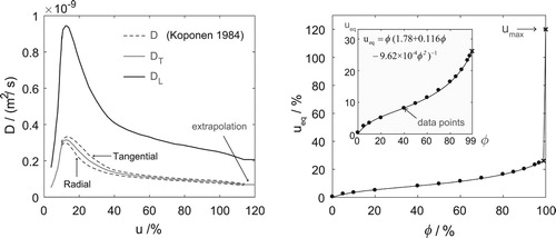
Table 1. Parameters used in the numerical model.

Equation		Value	Unit	Origin
4	$D_{\mathrm{u}}(u,T)$	–${}^{\mathrm{a}}$	m^2 s^−1	Koponen (1984)
5	$E_{\mathrm{A}}/R$	$-3400$	K	Koponen (1985)
6	$\phi \left(u_{\mathrm{e}\mathrm{q}}\right)$	–${}^{\mathrm{a}}$	%	Fredriksson and Thygesen (2017b)
6${}^{\mathrm{b}}$	$k_p$	15 or 30$\times {10}^{-9}$	kg m^−2 s^−1 Pa^−1	Wadsö (1993)${}^{\mathrm{c}}$
6	ρ	350	kg m^−3	Fredriksson et al. (2016)

${}^{\mathrm{a}}$ Values given in Figure 4.

${}^{\mathrm{b}}$ $15\times {10}^{-9}$ and $30\times {10}^{-9}$ kg m⁻² s⁻¹ Pa⁻¹ were used to model the laboratory and outdoor conditions, respectively.

${}^{\mathrm{c}}$Values were based on the literature review presented in the given reference.

The diffusion coefficient was determined on the basis of moisture gradients obtained under non-steady-state wetting conditions (Koponen 1984), and the values were thus deemed appropriate for use in the present study. The transversal diffusion coefficient, $D_T$, was taken as the mean value between the tangential and the radial directions, while the longitudinal diffusion coefficient, $D_L$ was set equal to $3\times D_{\mathrm{T}}$, as suggested by Koponen (1985).

The hygroscopic part of the sorption isotherm ($\phi <99$ %) was determined by fitting a Hailwood–Horrobin-type equation to experimental data from Fredriksson and Thygesen (2017b), which was obtained during absorption. The sorption isotherm was then extrapolated linearly up to the maximum moisture content at $\phi =100$%. The maximum moisture content at vacuum saturation is approximately 200% for Norway spruce. This moisture content is, however, unlikely to be reached in rain-exposed outdoor structures. For reference, Fredriksson and Lindgren (2013) measured a maximum moisture content of about 120–150% at the end-grain surface of Norway spruce sapwood specimens after 6.5 h of wetting. Because of this, in combination with that the diffusion coefficient data by Koponen (1984) extends to 120% moisture content, a value of $u_{\mathrm{m}\mathrm{a}\mathrm{x}}=120$% was chosen.

Based on a literature review by Wadsö (1993), mass transfer coefficients are generally measured in the range 1–30 $\times {10}^{-9}$ kg m⁻² s⁻¹ Pa⁻¹. Values of the mass transfer coefficient within this range were tested against the laboratory data, and the best fit was selected for use. This value was then increased by a factor of two when simulating the outdoor conditions, due to the higher wind velocity. The factor was based on the same literature review by Wadsö (1993), which suggests that the mass transfer coefficient increases by a factor of two when the wind velocity is increased from 0.2 m s⁻¹ (laboratory conditions) to 2 m s⁻¹ (average velocity in outdoor conditions).

The implications of assumptions and the choice of parameters are discussed further in Section 3.4.

2.4. Geometrical considerations and initial conditions

During wetting, any surfaces that were directly exposed to water are assumed to be wetted while any downwards-facing horizontal surfaces are assumed to remain dry. Contact areas between members where at least one edge was exposed to spraying are assumed to be fully wetted. It is further assumed that no interaction between areas of contact and the air may occur, including both the wood-to-wood and the PMMA-to-wood interfaces. Consequently, water is absorbed through exposed contact faces but are at the same time prevented from re-drying through the same face.

For the sake of practicality, a number of effects had to be either neglected or considered implicitly by the numerical model. Zero interaction with the air (i.e. $k_{\mathrm{p}}=0$) was assumed at any wood-to-wood interfaces, including those having an air gap of 2 mm. This assumption is reasonable in the case with direct contact but is conservative for the case with an air gap of 2 mm where the limited exchange of moisture with the air could potentially occur. In addition, any effects stemming from the transfer between the wet end-grain of the vertical board and the side-grain of the horizontal board, either through physical contact or via the air, were neglected. This assumption was necessary as any interaction between the two members would require simulation of end-grain absorption into the vertical board, a process which is highly uncertain. Finally, the boundary condition for wetting is assigned over a period corresponding to the duration of each spray sequence, whereas a residual film of water can potentially remain even after the spray is terminated.

The initial moisture content was set to $u_{\mathrm{e}\mathrm{q}}(\phi =65$%$)$, calculated from the sorption isotherm (Figure 4). The part of the horizontal board on the right side of the vertical board (see Figure 1) and the wood-to-wood interface were assumed to be fully wetted during spray, which was also supported by the measurements of the duration of surface moisture. The surface conditions on the left side of the vertical board were less well-defined. While this part of the board was sheltered from direct exposure to rain, it could still be wetted through water penetrating the gap. As the exact extent of liquid penetration through the gap is uncertain, the analysis was run twice; once with wetting limited to the right side and the gap ($x\ge -11\mathrm{m}\mathrm{m}$), and the other with an additional 20 mm on the left side of the vertical board subjected to wetting ($x\ge -31\mathrm{m}\mathrm{m}$). The sensitivity of the boundary condition on the outcome of the numerical solution was then analysed separately in Section 3.1.3.

3. Results and discussion

3.1. Laboratory experiment: single spray sequence

3.1.1. Moisture content distribution

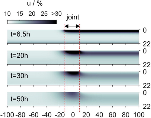
Figure 5 shows the numerical solution at four points in time ($t=$ 6.5, 20, 30 and 50 h) during and after the 6.5 h of spray. Note that the scale has been cut at u = 30%. Initially, directly after the spray sequence was terminated, a distinct region of elevated moisture content covered the segment of the upper boundary where wetting was assigned. A small gradient can be seen also at the bottom face of the board, this being due to vapour absorption from the damp air since the RH in the room was increased during the wetting sequence. After about 20 h, the outermost cell on the free segment of the upper surface had dried to about 15% while the moisture content in the interface area was maintained at a high level due to the zero-flux boundary condition being imposed. After 30 h, the effect of the joint was quite pronounced, which can be seen from the dark patch around the interface area. Finally, after 50 h, the entire specimen had dried below 30% moisture content but the residual moisture near the interface area was still distinguishable. Note that much moisture is redistributed from the sections near the joint to the dry volume of wood on the left side of the joint, this redistribution being affected by the boundary condition at $x\le -11\mathrm{m}\mathrm{m}$.

Figure 5. Moisture distributions at times 6.5, 20, 30 and 50 h, respectively, with wetting assigned to $x\ge -11$. Lengths are given in units of (mm).

3.1.2. Moisture content over time

Figure 6 shows the change in moisture content relative to the initial value of each time-series. The numerical solution in each point is presented as a range, where the upper and lower values differ in the size of the segment on the upper boundary that was subject to wetting. The experimental results include the measurements obtained from the joints designed without a gap. The joints designed with gap-sizes of 2 mm exhibited the same behaviour as the ones presented and have thus been omitted from the graph. In addition, the points along the section at x = −10 mm and x = 20 mm have been omitted, the former being treated separately in Section 3.1.3 due to them being very sensitive to the boundary condition on the left side of the vertical board. Each of the three sub-figures shows the change in moisture content on a specific depth at three different positions along the board. The timing and the amplitude of the peak values vary with depth, the response being increasingly damped with increasing depth. The distance relative to the joint also affects the response, where the peak values tend to decrease with increasing distance from the joint. The moisture content at a depth of 19 mm exhibited two distinct peaks, a large one in the beginning of the spray sequence and a smaller one after about 60 h. The first peak was caused by water vapour absorption through the bottom face of the board and the second peak was caused by moisture being transported from the upper face of the board.

Figure 6. Calculated and measured moisture content increase over the single 6.5 h spray sequence in the laboratory experiment. The first row of sub-figures shows the numerical solution and the second row shows the experimental results for slow-grown- and fast-grown wood, respectively.

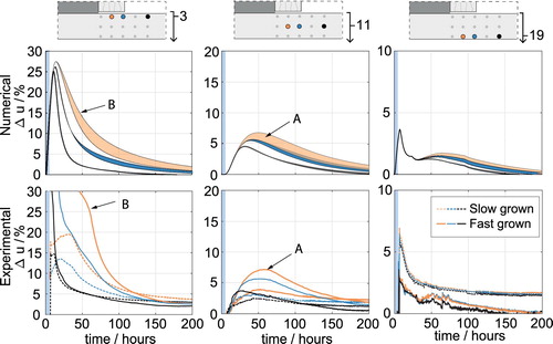
Overall, the main features of the numerical results were consistent with the experimental ones. Two notable discrepancies have been highlighted in Figure 6. The first one (marked as A) can be seen at a depth of 11 mm, where the measurements indicated a clear difference between x = 0 mm and x = 10 mm, which was only captured by one of the two simulations. This discrepancy is thus likely related to the boundary condition on the left side of the vertical board, and is discussed further in Section 3.1.3. The second discrepancy (marked as B), can be seen at a depth of 3 mm, where the moisture content of the fast-grown wood initially exceeds the simulated one by a wide margin. This is likely related to the model not being capable of fully describing capillary moisture transport, or due to the moisture sensor being completely enclosed by earlywood. Since the fast-grown wood specimens had very wide growth rings, the electrode was here positioned either in earlywood or in latewood, whereas for the slow grown wood the sensor was in contact with both wood types. Since the density of earlywood is lower than that of latewood, the moisture content of earlywood generally exceeds that of latewood when capillary water is absorbed. However, at lower moisture content when moisture uptake primarily occurs in cell walls, there is no difference in moisture content between latewood and earlywood (Fredriksson and Thygesen 2017a). Therefore, the difference seen here between fast-grown and slow-grown wood is most pronounced at the surface where the highest moisture contents occur.

3.1.3. Effects of the boundary conditions

The effect of the boundary condition on the left side of the joint (x < −11 mm) becomes increasingly pronounced in the points closer to the boundary in question. The points along the section at x = −10 mm are thus particularly sensitive to this effect, which is why they were omitted from the main analysis. The sensitivity of the numerical solution to the size of the wetted segment of the upper boundary was here evaluated.

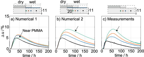
Figure 7(a,b) shows the two original solutions with the boundary conditions employed for the solutions presented in Figure 6, this time including also the points along x = −10 mm. Measurements on fast-grown wood in the corresponding points are shown in Figure 7(c). The point closest to the left edge of the vertical board (x = −11 mm) is extremely sensitive to the boundary condition, and a considerable effect was obtained by extending the wet segment from the left edge of the vertical board (x = −11 mm) to x = −31 mm (compare Figure 7(a,b)). The measured response in those points was consistent with the solution obtained by partially subjecting the upper surface to wetting (Figure 7(b)). Extending the wet segment more than 20 mm from the edge of the vertical board did, however, not have the same effect on the moisture content at the points of measurement in question.

Figure 7. Original numerical solutions (a,b) and measurements on fast-grown wood (c) during and after exposure to a single 6.5 h spray sequence. The top illustrations of the joint show the different boundary conditions as well as the location of the measuring points, where the colour of the measuring points and the corresponding data are equal.

It is difficult to predict exactly how a water film spreads through gaps and over a horizontal surface, as there are several potential mechanisms involved. Obviously, in the presence of a physical gap between the wooden members, then water will be able to penetrate the gap. In the case of direct wood-to-wood contact with no physical gap, then the same explanation is not entirely satisfying. Yet, the measurements indicated no significant difference between the joints having zero and 2 mm gap-sizes, which suggests that the direct wood-to-wood contact did not prevent wetting of the interface area. Modelling the exact mechanism by which water is distributed along horizontal surfaces and through gaps is, however, not critical to the problem in question, because in most practical situations it can be assumed that joints are subject to wetting on both sides of the connecting member, in which case it is reasonable to assume that the entire surface area is wetted.

3.1.4. Duration of surface moisture

The duration of surface moisture is given by Fredriksson et al. (2016) for the 6.5 h spray sequence, including measurements on free surfaces and the gaps. Measurements taken outside of the gap indicate that the surface remained visually wet for 4.2–12 h (median 8.8 h) after the spray sequence was terminated, with specimens made from slow-grown on the lower end of this range. This can be compared to the numerical solution where the saturation vapour pressure was maintained for 5.5 h after the spray. The sensors further indicated that water was present in the gap ($d=$ 2 mm) for 28 h (slow-grown) and 60 h (fast-grown), respectively, whereas the model gave a duration of 33 h. The measurements, as well as the comparison as a whole is subject to uncertainty. However, the inference that the joint effectively increased the time that the surface spent in the over-hygroscopic range, and that this increase shows some similarity to the measured surface moisture data, is still valid. This indicates that the simplified boundary conditions employed show some resemblance to the actual conditions on the surface. Interesting to note is that the measurements did not show a significant difference between free surfaces of vertical and horizontal boards. Although surprising, the longer durations of surface wetness on free surfaces can thus not be explained by residual standing water.

3.2. Laboratory experiment: cyclic spray sequence

Figure 8 shows the results for the cyclic spray sequence. The difference between the fast-grown and the slow-grown wood was here smaller, and the results were in relatively good agreement with the experimental data. The largest discrepancies can be observed in the vicinity of the interface area in Figure 8 where the numerical model underestimates the timing of the peak value after the first spray cycle. The subsequent spray cycles were, however, consistent with the experimental data.

Figure 8. Measured and calculated moisture content increase over the cyclic spray sequence. The first row of subfigures shows the numerical solution and the second row shows the experimental results for slow-grown- and fast-grown wood, respectively.

Despite minor discrepancies, the performance of the numerical model was deemed sufficient for the application. The results indicate that the spatial distribution of moisture in the near vicinity of moisture traps can, in fact, be simulated, with reasonable accuracy, by employing a simple diffusion model with appropriate boundary conditions adapted for wetting and zero-flux boundary conditions along areas of contact. It should be emphasized, however, that the moisture profile in the over-hygroscopic region remains uncertain.

3.3. Outdoor exposure

3.3.1. Moisture content over time

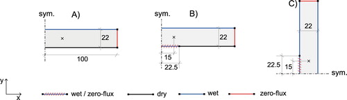
The horizontal board (A) and the two joints (B and C) previously shown in Figure 2 were modelled with the boundary conditions and the geometries shown in Figure 9. The total length of each board was set to 200 mm to reduce the computational time. In addition, axial symmetry was used in all three cases. Transport in the z-direction was neglected since the boundary condition along the z-direction was uniform and the width of the board (90 mm) was about four times larger than the thickness (22 mm), with the point of interest being located at half the width of the board. It was assumed that the entire interface area of the joints and any vertical/top surfaces were fully wetted during rain events, which is a conservative scenario. As such, the model should generally overestimate the effects of precipitation on the moisture content.

Figure 9. Geometry of the horizontal board (A) and the two types of joints (B and C), their boundary conditions and the point in each geometry that was probed (cross). Lengths given in units of (mm).

Figure 10 shows the numerical and experimental results for the horizontal board (A) and the two joints (B and C), respectively. The moisture content variation of the joints is shown as areas, where each area encloses the moisture content of the two replicates. The model captured the seasonal variation of the horizontal board but gave larger peaks during periods with high amounts of precipitation. As previously stated, this discrepancy can be related to the conservative boundary conditions. In addition, the smaller rain-induced fluctuations could be related to the material in question having lower permeability than plain sapwood, as neither heartwood-content nor density was documented. A more detailed analysis on the free horizontal board, including sources of error, model accuracy and surface conditions can be found in Niklewski et al. (2016). Qualitatively, the model captured the increased difference between the horizontal board and the two joints during periods with high amounts of precipitation.

Figure 10. Experimental results (left) and numerical results (right) for the joints exposed outdoors. The areas between the curves for the experimental data represents the variation of two specimens.

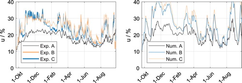
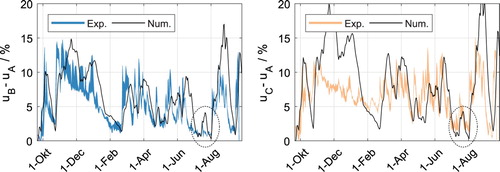
3.3.2. The effect of the joint

The effect of the joint can be isolated by subtracting the moisture content of the horizontal board ($u_{\mathrm{A}}$) from the moisture content of the joints ($u_{\mathrm{B}}$ and $u_{\mathrm{C}}$). The difference between two moisture content values is less sensitive to systematic measurement errors and is, therefore, more suitable as a basis for evaluation than absolute moisture content values. Figure 11 shows the difference in moisture content between each of the two joints (B and C) and the free horizontal board (A). Qualitatively, the numerical results for joint B were quite consistent with the measurements, both with respect to overall behaviour and magnitude. In some cases, the difference between board A and joint B did not increase during precipitation (see dotted circle) whereas joint C responded more consistently to precipitation. This is likely related to the fact that the contact area of joint B was partially sheltered by the horizontal board. In general, the difference between the two joints was small, as predicted numerically and measured experimentally. The moisture content of joint C was, on average, slightly higher than that of B. However, the numerical result for joint C was overall less consistent with the measurements, especially during the first months. Considering the many uncertainties involved in the analysis, the numerical analysis was remarkably adequate.

Figure 11. The difference between the moisture content of the two joints ($u_{\mathrm{B}}\mathrm{a}\mathrm{n}\mathrm{d}{u}_C$) and that of the free horizontal board ($u_{\mathrm{A}}$).

3.3.3. Time above 25% moisture content

The time above 25% moisture content is frequently employed to evaluate the susceptibility of wood to decay growth (see Rapp et al. 2000; Isaksson and Thelandersson 2013). Figure 12 shows how the duration above 25% moisture content is distributed in the horizontal board and the two joints. As indicated by the lighter patches near the interface areas, the exposure is greatly affected by the contact area. The results also imply that the decay assessment is strongly dependent on the spatial location of the measurements. For a free horizontal board (A), the moisture conditions are most severe near the exposed surface. The risk is, however, most pronounced in the section at the joint (x = 0 mm), where the time above 25% moisture content was 100–300 days depending on the distance from the exposed surface (Figure 12( B,C)).

Figure 12. The distribution of time above 25% moisture content in the horizontal board (A) and the two joints (B) and (C). Lengths given in units of (mm).

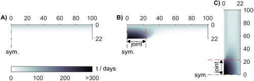
The results indicate that the moisture conditions necessary for the growth of fungal decay were maintained almost permanently in the vicinity of the joint, despite the fact that the joint itself was exposed to only moderate amounts of precipitation. Provided that the duration above 25% is a good indicator for decay rate, these results would suggest that the decay rate would not increase considerably even if the moisture conditions were made worse, i.e. by increasing the exposure to precipitation or by increasing the area of contact. This would also imply that the design of joints is more decisive in climates with low amounts of precipitation, where the wood can dry out between rain events. Although possibly coincidental, Groot (1992) did not find any significant relation between the design of the assembly and the rate of decay growth in a tropical climate, whereas an effect was found in a temperate climate.

3.4. Final remarks on the model

The rate of absorption during wetting depends on the diffusion coefficient and the maximum moisture content assigned on the boundary. The absorption rate is linearly proportional to the square root of time, with a constant of proportionality in the range 2–4 g m${}^{-2}{\mathrm{s}}^{-1/2}$) (Niemz et al. 2010) for Norway spruce side-grain. This can be compared to the numerical model that yields a value of approximately 4.2 g m${}^{-2}{\mathrm{s}}^{-1/2}$), at 20${}^{\circ }$C with an initial moisture content of 12%. The high value was deemed acceptable as the material involved in the laboratory experiment consists exclusively of low-density sapwood.

While the volume of absorbed water is sufficiently accurate, the shape of the moisture profile at the exposed boundary remains uncertain. End-grain absorption experiments by Lindgren (1991) show the formation of a moisture plateau, at about 80–90% moisture content, after 20 h wetting. This type of plateau cannot be reproduced by the diffusion coefficient employed in the present study. Moisture profiles obtained during side-grain wetting (see Lindgren 1991; Dvinskikh et al. 2011) instead exhibit diffusion-like moisture profiles, likely due to the overall lower moisture levels obtained. As such, the model is not suitable for modelling end-grain absorption nor very long wetting periods when the capillary region extends beyond the surface layer.

The mass transfer coefficient, $k_{\mathrm{p}}$, was assumed to be independent on moisture content. For wood, it has, however, been shown that the mass transfer coefficient tends to increase with increasing moisture content (Siau and Avramidis 1996). Describing this moisture-dependency is, however, non-trivial, in particular with vapour pressure as the driving potential (Tremblay et al. 2000). The constant $k_{\mathrm{p}}$ employed in the present study thus overestimates the surface flux at low moisture content and underestimate the surface flux at high moisture content. The latter is to some extent counteracted by neglecting the effect of evaporative cooling, which causes $p_{\mathrm{v}\mathrm{s}}$ as well as the corresponding surface flux, to decrease.

4. Conclusions

The overall good agreement between numerical and experimental results suggests that the moisture behaviour of the joints in the present study can be described by employing appropriate boundary conditions for the inhibited drying in contact areas. The moisture behaviour was well described by employing a zero-flux boundary condition on interface areas during drying, while simultaneously allowing absorption of liquid water. Due to the simplified representation of free water transport, the model accuracy decreased when the moisture content entered the over-hygroscopic region. However, as the duration of moisture contents in the over-hygroscopic region was still reproduced with reasonable accurately, the model remains useful for durability applications where the time at high moisture contents is considered as one of the most important durability-indicators.

Acknowledgments

The authors would like to thank Tord Isaksson for providing experimental data.

Disclosure statement

No potential conflict of interest was reported by the authors.

Additional information

Funding

The second author would like to acknowledge the funding received from the Swedish Research Council Formas (Svenska Forskningsrådet Formas) (grant number: 2013-1024).

References

- Angst, V. and Malo, K. A. (2010) Moisture induced stresses perpendicular to the grain in glulam: Review and evaluation of the relative importance of models and parameters. Holzforschung, 64(5), 609–617.
- Brischke, C. and Thelandersson, S. (2014) Modelling the outdoor performance of wood products – A review on existing approaches. Construction and Building Materials, 66, 384–397.
- Brischke, C., Bayerbach, R. and Otto Rapp, A. (2006) Decay-influencing factors: A basis for service life prediction of wood and wood-based products. Wood Material Science and Engineering, 1(3–4), 91–107.
- Brischke, C., Meyer-Veltrup, L. and Bornemann, T. (2017) Moisture performance and durability of wooden façades and decking during six years of outdoor exposure. Journal of Building Engineering, 13, 207–215.
- Comstock, G. and Côté, W. (1968) Factors affecting permeability and pit aspiration in coniferous sapwood. Wood Science and Technology, 2(4), 279–291.
- De Meijer, M. and Militz, H. (2000) Moisture transport in coated wood. Part 1: Analysis of sorption rates and moisture content profiles in spruce during liquid water uptake. Holz als Roh-und Werkstoff, 58(5), 354–362.
- Derbyshire, H. and Robson, D. J. (1999) Moisture conditions in coated exterior woodpart 4: Theoretical basis for observed behaviour. A computer modelling study. Holz als Roh- und Werkstoff, 57(2), 105–113.
- Dvinskikh, S. V., Furó, I., Sandberg, D. and Söderström, O. (2011) Moisture content profiles and uptake kinetics in wood cladding materials evaluated by a portable nuclear magnetic resonance spectrometer. Wood Material Science & Engineering, 6(3), 119–127.
- Fredriksson, M. and Lindgren, O. (2013) End grain water absorption and redistribution in slow-grown and fast-grown Norway spruce (Picea abies (L.) Karst.) heartwood and sapwood. Wood Material Science & Engineering, 8(4), 245–252.
- Fredriksson, M. and Thygesen, L. G. (2017a) The states of water in Norway spruce (Picea abies (L.) Karst.) studied by low-field nuclear magnetic resonance (LFNMR) relaxometry: Assignment of free-water populations based on quantitative wood anatomy. Holzforschung, 71(1), 77–90.
- Fredriksson, M. and Thygesen, L. G. (2017b) The states of water in Norway spruce (Picea abies (L.) Karst.) studied by low-field nuclear magnetic resonance (LFNMR) relaxometry: Assignment of free-water populations based on quantitative wood anatomy. Holzforschung, 71(1), 77–90.
- Fredriksson, M., Wadsö, L. and Johansson, P. (2013) Methods for determination of duration of surface moisture and presence of water in gaps in wood joints. Wood Science and Technology, 47(5), 913–924.
- Fredriksson, M., Wadsö, L., Johansson, P. and Ulvcrona, T. (2016) Microclimate and moisture content profile measurements in rain exposed Norway spruce (Picea abies (L.) Karst.) joints. Wood Material Science & Engineering, 11(4), 189–200.
- Gaby, L. I. and Duff, J. E. (1978) Moisture content changes in wood deck and rail components. USDA Forest Service Research Paper SE (USA).
- Groot, R. C. D. (1992) Test assemblies for monitoring decay in wood exposed above ground. International Biodeterioration & Biodegradation, 29(2), 151–175.
- Hjort, S. (1996) Full-scale method for testing moisture conditions in painted wood paneling. Journal of Coatings Technology, 68(856), 31–39.
- Isaksson, T. and Thelandersson, S. (2013) Experimental investigation on the effect of detail design on wood moisture content in outdoor above ground applications. Building and Environment, 59, 239–249.
- Kang, W., Lee, Y. H., Chung, W. Y. and Xu, H. L. (2009) Parameter estimation of moisture diffusivity in wood by an inverse method. Journal of Wood Science, 55(2), 83–90.
- Koponen, H. (1984) Dependences of moisture diffusion coefficients of wood and wooden panels on moisture content and wood properties. Paperi ja puu, 66(12), 740–745.
- Koponen, H. (1985) Dependence of moisture transfer and diffusion coefficients on temperature. Paperi ja puu, 8, 428–439.
- Kumaran, M. (1999) Moisture diffusivity of building materials from water absorption measurements. Journal of Thermal Envelope and Building Science, 22(4), 349–355.
- Lindgren, O. (1991) Utilization of computer axial tomography and digital image processing for studies of moisture sorption into wood. Trtek Report, Stockholm, Sweden, 1991 (in Swedish).
- Meyer, L., Brischke, C. and Preston, A. (2016) Testing the durability of timber above ground: A review on methodology. Wood Material Science & Engineering, 11(5), 283–304.
- Meyer-Veltrup, L., Brischke, C., Niklewski, J. and Frühwald Hansson, E. (2018) Design and performance prediction of timber bridges based on a factorization approach. Wood Material Science & Engineering, 0(0), 1–7.
- Niemz, P., Mannes, D., Herbers, Y. and Koch, W. (2010) Untersuchungen zum wasseraufnahmekoeffizienten von holz bei variation von holzart und flüssigkeit. Bauphysik, 32(3), 149–153.
- Niklewski, J., Fredriksson, M. and Isaksson, T. (2016) Moisture content prediction of rain-exposed wood: Test and evaluation of a simple numerical model for durability applications. Building and Environment, 97, 126–136.
- Niklewski, J., Isaksson, T., Frühwald Hansson, E. and Thelandersson, S. (2018) Moisture conditions of rain-exposed glue-laminated timber members: The effect of different detailing. Wood Material Science & Engineering, 13(3): 129–140.
- Norberg, P. (1999) Monitoring wood moisture content using the wetcorr method. Part 1: Background and theoretical considerations. Holz als Roh- und Werkstoff, 57(6), 448–453.
- Perre, P., Moser, M. and Martin, M. (1993) Advances in transport phenomena during convective drying with superheated steam and moist air. International Journal of Heat and Mass Transfer, 36(11), 2725–2746.
- Rapp, A., Peek, R. D. and Sailer, M. (2000) Modelling the moisture induced risk of decay for treated and untreated wood above ground. Holzforschung, 54(2), 111–118.
- Robbers, K., Fromm, J. and Melcher, E. (2018) Evaluation of pedestrian timber bridges in the city of hamburg with particular consideration of design detailing. Wood Material Science & Engineering, 0(0), 1–10.
- Siau, J. F. and Avramidis, S. (1996) The surface emission coefficient of wood. Wood and Fiber Science, 28(2), 178–185.
- Simpson, W. T. (1993) Determination and use of moisture diffusion coefficient to characterize drying of northern red oak (quercus rubra). Wood Science and Technology, 27(6), 409–420.
- Skaar, C. (1964) Some factors involved in the electrical determination of moisture gradients in wood. Forest Products Journal, 14, 239–243.
- Spolek, G. A. and Plumb, O. A. (1981) Capillary pressure in softwoods. Wood Science and Technology, 15(3), 189–199.
- Stamm, A. (1964) Wood and Cellulose Science. American Association for the Advancement of Science (New York: Ronald Press).
- Tremblay, C., Cloutier, A. and Fortin, Y. (2000) Experimental determination of the convective heat and mass transfer coefficients for wood drying. Wood Science and Technology, 34(3), 253–276.
- Virta, J., Koponen, S. and Absetz, I. (2006) Modelling moisture distribution in wooden cladding board as a result of short-term single-sided water soaking. Building and Environment, 41(11), 1593–1599.
- Wadsö, L. (1993) Surface mass transfer coefficients for wood. Drying Technology, 11(6), 1227–1249.
- Zelinka, S. L., Wiedenhoeft, A. C., Glass, S. V. and Ruffinatto, F. (2015) Anatomically informed mesoscale electrical impedance spectroscopy in southern pine and the electric field distribution for pin-type electric moisture metres. Wood Material Science & Engineering, 10(2), 189–196.