Numerical study on the effects of macro climate and detailing on the relative decay hazard of Norway spruce

ABSTRACT

The durability of wood depends on its in-use environmental conditions. The aim of this study was to estimate the effects associated with macro climate and detail design as well as their interdependence. A numerical moisture model and two different decay prediction models were utilized for assessing the decay risk of a horizontal member and a joint exposed at 300 sites scattered across Europe. In general, the results obtained with both decay models exhibited strong similarities to the Scheffer climate index. Distinct discrepancies were however observed in regions with much precipitation where one model stood out as less dependent on precipitation and more dependent on relative humidity. The projected decay rate of the joint was about two to four times higher than that of the horizontal board, depending on the model employed. One of the models indicated that the relative difference between the horizontal member and the joint decreased with increasing amounts of precipitation. Due to lack of reliable experimental data, no inference regarding the model accuracy could be made. Future studies should focus on collecting empirical data on relative decay risk in different climates, preferably focusing on regions where the difference in projected decay depends on the model employed.

KEYWORDS:

• Wood
• moisture transport
• decay hazard
• climate
• detailing
• performance-based design

1. Introduction

Wood is susceptible to a variety of degrading organisms such as termites, beetle larvae and decay fungi. Infestation by decay fungi is one of the most frequent modes of biological degradation in outdoor above-ground applications, particularly in the northern hemisphere. The service life expectancy of wooden members depends on the material's intrinsic properties, such as chemical composition and moisture dynamics, and on their in-service environmental conditions.

The current standard for durability requirements, EN460 (1994), distinguishes between durability class (EN350, 2016) and hazard class (EN335-1, 2006), where the former is a measure of the material's natural resistance to decay and the latter is related to the severity of the site-specific environmental conditions. The more recent EN335 (2013) replaced the term hazard class by use-class (UC) and revised their definitions. UC 3, which refers to rain-exposed wood above ground, is further separated into subclasses UC 3.1 and UC 3.2, depending on the ability of the wood to dry out subsequent to wetting.

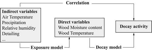
Environmental variables can be characterized as indirect or direct, where the direct variables are dependent on the indirect ones (Brischke et al., 2006). Direct environmental variables include the wood moisture content and the wood temperature, which depend upon indirect variables such as precipitation, air temperature and design of details. Service life models based on indirect environmental variables are fundamentally different from those based on direct environmental variables in that they lack the intrinsic connection to decay activity (see Figure 1). For predictive use, models based on direct variables need to first estimate their input on the basis of the indirect variables, a process which is hereafter denoted exposure modelling.

Figure 1. Relationship between indirect variables, direct variables and decay rate.

The earliest model to quantify the effect of indirect environmental variables on wood decay was developed by Scheffer (1971), who established an empirical relationship between frequency of precipitation, air temperature and wood decay. Similar models have later been developed, including those involving driving rain (Cornick and Dalgliesh, 2003), condensation (Fernandez-Golfin, 2016) and design of details amongst other parameters (Wang et al., 2008).

Models that are based on direct environmental variables build on the relationship between the decay activity and the moisture and temperature conditions of the material to which the organisms are exposed (see e.g. Isaksson et al., 2013; Brischke and Meyer-Veltrup, 2016; Viitanen, 1997; Saito et al., 2012). For predictive use, such models rely on the exposure model so as to obtain useful input data (see e.g. Viitanen et al. , 2010; Saito et al., 2012; Niklewski et al., 2016a). This concept has previously been used to establish a factorized design framework for wood durability (Meyer-Veltrup et al. , 2018), which has been used in recent works on design guidelines for wood in above-ground applications (Isaksson et al., 2013) and timber bridges (Thelandersson, 2017). Factorization implies that the decay assessment is described as the product of various factors, where each factor is a relative measure of service life. The focus of this study is to quantify the relative effect of geographical exposure site and detail design.

Recent efforts have been made to quantify the decay hazard of European climates through direct environmental variables. The first such decay hazard maps were presented by Brischke et al. (2011) who integrated an empirical exposure model with two different models for decay activity. The exposure model that was employed lacked spatial resolution, had limited experimental verification and was limited to horizontal boards. A new set of decay hazard maps were later presented by Niklewski et al. (2016), where a numerical one-dimensional moisture transport model was coupled with a decay model so as to obtain a measure on spatial distribution of decay risk in the wood cross section. The model was, however, still limited to one-dimensional geometries.

The one-dimensional moisture transport model employed by Niklewski et al. (2016a) was recently extended to two-dimensional moisture transport in an effort to describe the behaviour of details such as the one shown in Figure 2 (Niklewski and Fredriksson, 2019). Similar numerical moisture transport models have frequently been used to describe the moisture behaviour of wooden boards exposed to water (see e.g. Niklewski et al., 2016a; Virta et al., 2006; Derbyshire and Robson, 1999; De Meijer and Militz, 2000). However, to the authors' knowledge, no such model has successfully been applied on more complex geometries, such as joints. Being able to model the impact of joints on the moisture behaviour is crucial in durability applications, as the damp conditions between members facilitate decay growth.

Figure 2. Design geometries referring to UC 3.1 (top) and UC 3.2 (bottom) according to EN335 (2013).

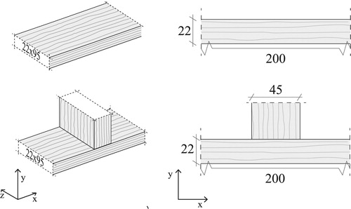
The objective of this study is twofold. First, the study aims to provide updated decay hazard maps based on the performance based approach. The second objective is to find potential nonlinear effects between macro climate, detail design and relative decay hazard. The numerical exposure model utilizes a two-dimensional numerical exposure model with material parameters for Norway spruce sapwood. Variations in material climate are calculated for more than 300 different geographical sites across Europe. The data is then fed into a decay model, which is used to calculate the decay rate of the member in question. The calculations were performed on two specific specimen designs, including a horizontal board and a connection detail (see Figure 2). The conditions involved can be seen as representing wood exposed outdoors, freely weathered above ground with (UC 3.1) and without (UC 3.2) a risk of moisture accumulation, respectively, according to the definitions given by EN335 (2013).

2. Materials and methods

2.1. Model overview

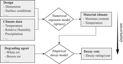
The coupling between the numerical model for moisture transport and the decay model is shown in Figure 3, where the lower level is fed data from the upper level. The numerical model calculates the moisture variation of a wooden member of a certain design and climate. The output is then fed to the decay model where the risk of fungal decay is quantified. Note that the wood species is not a variable input to the numerical model, which is due to the model being limited to Norway spruce as reflected by its set of parameters.

Figure 3. Workflow from indirect variables to decay rate. Note that the numerical exposure model of the present paper is limited to Norway spruce.

Figure 2 shows the two different specimen designs that were used for simulation tests. The first design is a board ($22\times 95$ mm²) with sealed end-grain, oriented horizontally and located above ground with one side being exposed to precipitation and the other side being sheltered. The second specimen consists of the same board, connected by its upper face to the end-grain of a secondary member ($45\times 95$ mm²). Studies by Niklewski et al. (2017) and Isaksson et al. (2013) have shown that the moisture conditions of different joints are quite similar, as long as exposed end-grain is not present. The joint modelled as part of the present study can therefore be said to represent wood in UC 3.2 where transverse moisture uptake is dominant.

The theoretical basis for the numerical model is described in Section 2.1.1, with experimental validation provided in a separate publication (see Niklewski and Fredriksson, 2019). The two specific designs were selected as they have previously exhibited predictable behaviour when exposed to water. The decay models are described briefly in Section 2.1.2.

2.1.1. Numerical model

The moisture flux within a wooden member can be described by Fick's second law of diffusion. With the moisture content gradient as the driving potential, its two-dimensional form is written as follows:(1) $\begin{array}{rll}\frac{\mathrm{\partial }u}{\mathrm{\partial }t}& =\mathrm{\nabla }\left(D_u\mathrm{\nabla }u\right),& \\ \mathrm{\nabla }& =\left(\frac{\mathrm{\partial }u}{\mathrm{\partial }x},\frac{\mathrm{\partial }u}{\mathrm{\partial }y}\right),\end{array}$(1) where ${\mathit{D}}_{\mathit{u}}$(m²/s) is a diagonal matrix with diffusion coefficients of two orthogonal directions. The rate of moisture transport generally decreases with decreasing temperature. This effect can be considered by adjusting the diffusion coefficient according to the Arrhenius equation (Simpson, 1993):(2) ${\mathit{D}}_u\left(T\right)={\mathit{D}}_0{\mathrm{e}}^{-E_A/\left(R\right(T+273.15\left)\right)},$(2) where ${\mathit{D}}_{\mathbf{0}}$ is the base value, ${\mathit{D}}_{\mathbf{u}}$ is the temperature-adjusted diffusion coefficient, $E_A$ is the activation energy, R the universal gas constant and T is the temperature.

The transport coefficient is subject to a certain degree of uncertainty, in particular with respect to the shape of the moisture profile within the over-hygroscopic region. Since the over-hygroscopic region is normally limited to the surface during short to medium wetting periods, large errors in the near vicinity of the surface are expected. The exact shape of the moisture profile is however less important, granted that the duration spent in the over-hygroscopic region is modelled with sufficient accuracy.

The moisture exchange with the environment, $q_n\left({\mathrm{k}\mathrm{g}/(\mathrm{m}}^2\mathrm{s})\right)$, is described as follows:(3) $q_n=k_p(p_{vs}-p_{va}),$(3) where $k_p\left({\mathrm{k}\mathrm{g}/(\mathrm{m}}^2\mathrm{s}\mathrm{P}\mathrm{a})\right)$ is the mass transfer coefficient, $p_{va}\left(\mathrm{P}\mathrm{a}\right)$ is the vapour pressure of the air and $p_{vs}\left(\mathrm{P}\mathrm{a}\right)$ is the vapour pressure on the wood surface. It is implied that the vapour pressure on the wood surface is in equilibrium with the moisture content at the same location and the vapour pressure on the wood surface may thus be obtained directly from the sorption isotherm. When the wood surface is exposed to liquid water it can be assumed that the surface resistance is small (De Meijer and Militz, 2000) and that the outermost fibres are instantly saturated (Salin, 2008). It was here assumed that the surface immediately assumes its maximum value when wetted. The contact area was considered by neglecting any interaction between the air and the wood–wood interface area while absorption of free water through the same surface was allowed.

All parameters are listed in Table 1 with reference to their origin. The diffusion coefficients for longitudinal and transversal moisture transport as well as the sorption isotherm are given in Figure 4. The longitudinal diffusion coefficeint was assumed to be three times higher than the transversal one, as suggested by Koponen (1985). The hygroscopic part of the sorption isotherm is based on measurements by Fredriksson and Thygesen (2017), which have been extrapolated up to $\phi =99\text{\%}$ and then interpolated in the range $\phi =99-100\text{\%}$. The maximum moisture content at $\phi =100\text{\%}$ was set to $u=120\text{\%}$, partly because the diffusion coefficients by Koponen (1984) are limited to moisture contents below $u=120\text{\%}$.

Figure 4. Left: diffusion coefficients, $D_u$, based on measurements by Koponen (1984) as functions of moisture content, u. Right: equilibrium moisture content, $u_{eq}$, as a function of relative humidity, φ, with filled markers showing the data points from Fredriksson and Thygesen (2017).

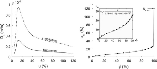
Table 1. Parameters used in the numerical model with reference to their origin.

Eqs.			Value	Unit	Origin
1	$D_{\mathrm{u}}$	Diffusion coeff.	${-}^{\mathrm{a}}$	m^2/s	(Koponen, 1984)
2	$E_A$	Activation energy	6750	cal/mol	(Koponen, 1985)
3	$u_{\mathrm{e}\mathrm{q}}\left(\phi \right)$	Sorption isotherm	${-}^{\mathrm{a}}$	%	(Fredriksson and Thygesen, 2017)
3	$k_p$	Mass transfer coeff.	30$\times {10}^{-9}$	kg/(m^2s Pa)	(Wadsö, 1993)
3	ρ	Wood density	350	kg/m^3	(Fredriksson et al., 2016)

^aValues given in Figure 4.

2.1.2. Modelling decay

In this study, the dosimeter concept proposed by Brischke and Rapp (2008) was used as a quantitative measure on decay risk. The equations are derived from a data set where double layer setups were exposed to outdoor climate over several years, while their moisture content, temperature and decay rating were monitored. Brischke and Rapp (2008) established a relationship between decay rating and daily averages of moisture content and temperature through use of a concept of moisture content and temperature induced doses, a dose being a value between 0 and 1 where higher values imply more favourable conditions for decay growth. The moisture content and temperature induced doses are combined to a single daily dose that describes the conditions for decay on that day. Daily doses are accumulated over time until a critical threshold is exceeded which corresponds to a certain decay rating.

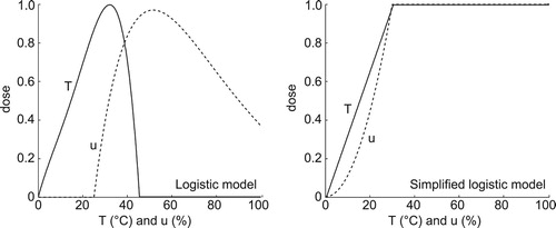
The same dataset has later been revisited, and a number of different dose models have been proposed by Brischke and Rapp (2010), Isaksson and Thelandersson (2013) and Brischke and Meyer-Veltrup (2016). The models primarily differ in how the moisture content and temperature relate to their corresponding dose. Here, two different models developed by Isaksson and Thelandersson (2013) and Brischke et al. (2013) were used, namely the logistic model (LM) and the simplified logistic model (SLM). The governing functions are shown in Figure 5, where the daily moisture content ($d_u$) and temperature ($d_T$) induced doses are calculated from the daily averages of wood moisture content and temperature, respectively. The function $d_T\left(T\right)$ of the logistic model is conditional and is not valid when the temperature at any point in a given day exceeds ${40}^{\circ }$C or falls below $0^{\circ }$C , in which case $d_T$ is set to zero. The daily dose, $d_{\mathrm{d}\mathrm{a}\mathrm{y}}$, is calculated by combining the two doses in question. The SLM weights the effect of moisture and temperature equally, with the daily dose being calculated as the product of the moisture- and temperature induced doses, according to (4) $d_{\mathrm{d}\mathrm{a}\mathrm{y}}=\left\{\begin{array}{cc}{d}_u\times d_T,& \mathrm{i}\mathrm{f}{d}_u>0\mathrm{a}\mathrm{n}\mathrm{d}{d}_T>0,\\ 0,& \mathrm{o}\mathrm{t}\mathrm{h}\mathrm{e}\mathrm{r}\mathrm{w}\mathrm{i}\mathrm{s}\mathrm{e}.\end{array}\right.$(4) The LM applies more weight to the temperature, with the daily dose being calculated as follows:(5) $d_{day}=\{\begin{array}{cc}(3.2\times d_T+d_u)/4.2,& \mathrm{i}\mathrm{f}{d}_u>0\mathrm{a}\mathrm{n}\mathrm{d}{d}_T>0,\\ 0,& \mathrm{o}\mathrm{t}\mathrm{h}\mathrm{e}\mathrm{r}\mathrm{w}\mathrm{i}\mathrm{s}\mathrm{e}.\end{array}$(5) Finally, an empirical equation connects the accumulated dose to a corresponding decay rating, where the decay rating is described on a scale from 0 (no decay) to 4 (failure) according to EN252 (2015). The critical dose corresponding to decay rating 1 (slight decay) is approximately 230 for brown rot (Brischke and Meyer-Veltrup, 2016), with the exact value being dependent on the dose-model employed.

Figure 5. Models describing the moisture content and temperature induced dose, respectively, as functions of daily average moisture content, u, and daily average temperature, T.

In this study, the annual dose is used as a measure on the decay hazard, defined according to Equation (6(6) $d_{\mathrm{y}\mathrm{e}\mathrm{a}\mathrm{r}}=\sum _{i=1}^{365}{d}_{\mathrm{d}\mathrm{a}\mathrm{y},i}.$(6) ). The annual dose is inversely proportional to the time until a certain decay rating is reached. Consequently, the relative difference between two doses is equal to their relative decay rate. For example, increasing the annual dose by a factor of two implies that the time until a certain decay rating is reached is reduced by 50%, granted that the same weather is repeated every year.(6) $d_{\mathrm{y}\mathrm{e}\mathrm{a}\mathrm{r}}=\sum _{i=1}^{365}{d}_{\mathrm{d}\mathrm{a}\mathrm{y},i}.$(6) The equations governing the logistic model stem from the relationship between biological activity and environmental variables whereas the simplified logistic model is more empirical in nature. From a physical viewpoint, the logistic model is more sound. However, the simplified model addresses certain issues related to the input data, such as uncertainty related to its acquisition. In practice, it is difficult to probe the exact location where decay will develop. One problem is that decay is difficult to predict, as it often begins to grow in cracks and other imperfections where the local conditions differ from those of the intact specimen. Another problem is that decay generally develop on wood surfaces, where the moisture content is difficult to probe without disrupting the conditions. Instead, the moisture content is often probed in accessible locations, e.g. at some distance from the exposed surface. As the measured moisture content then differs from the conditions where decay develops, the logistic model is not easily applicable.

2.2. Scheffer index

The Scheffer climate index (SCI) is employed as a comparative measure on the relative decay hazard in different climates. Scheffer (1971) established an empirical relationship between macro climate and decay rate, described as follows:(7) $\mathrm{C}\mathrm{l}\mathrm{i}\mathrm{m}\mathrm{a}\mathrm{t}\mathrm{e}\mathrm{i}\mathrm{n}\mathrm{d}\mathrm{e}\mathrm{x}=\sum _{Jan}^{Dec}\frac{(T-2)(t-3)}{16.7},$(7) where T (${}^{\circ }$C) and t (days) are the mean monthly temperature and the number of days in a month with more than 0.25 mm of precipitation. The Scheffer index is based on a dataset consisting of (1) decay rating of flooring boards and post-rails exposed at different geographic locations and (2) macro climate conditions on each site. Equation (7(7) $\mathrm{C}\mathrm{l}\mathrm{i}\mathrm{m}\mathrm{a}\mathrm{t}\mathrm{e}\mathrm{i}\mathrm{n}\mathrm{d}\mathrm{e}\mathrm{x}=\sum _{Jan}^{Dec}\frac{(T-2)(t-3)}{16.7},$(7) ) is a purely empirical model describing the relative decay hazard of different climates. Because the index is relative, it is has been widely used as a measure of regional decay risk. However, it is not capable of calculating decay rates in absolute terms.

2.3. Model coupling

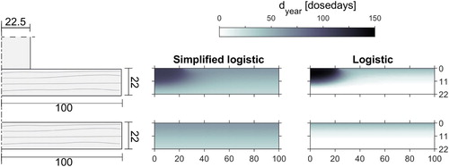
Decay generally develops where the conditions are most favourable. For example, when only one face of a member is exposed to precipitation, then decay is unlikely to develop on the opposite side. As such, to some extent decay growth can be predicted by finding the location where the conditions are most favourable, as indicated by the maximum dose.

Figure 6 shows the spatial distribution of accumulated dose, calculated for the board and the joint, respectively. The annual dose is nonuniformly distributed, with higher values near the exposed face and in the vicinity of the joint where decay is likely to develop. The logistic model yields zero doses in large regions of the specimens, which is due to the daily moisture content never exceeding 25% in those regions. Conversely, the simplified logistic model gives doses in the entire cross section, including the region near the bottom surface which is not directly exposed to precipitation.

Figure 6. Distribution of annual dose, calculated from a normal year of weather data in Bischofshofen, Austria.

Two different definitions were employed so as to obtain an explicit measure on decay hazard. The first definition (hereafter denoted D${}_1$ ) follows the method used by Thelandersson et al. (2011), where the decay hazard is calculated through use of the simplified logistic model with input obtained at a fixed depth of 10 mm from the exposed wood surface. The second definition (hereafter denoted D${}_2$) is based on the logistic model, where it is assumed that decay begins where the conditions are most favourable, which is the location having the highest dose.

2.4. Weather data and mapping

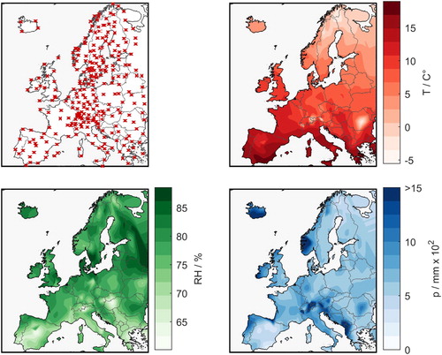
Macro climates for 300 different locations spread across Europe, obtained through the Meteonorm database, were used for the modelling. The macro climate on each location was described by a normal year, which is based on a stochastic model of the weather between 1963 and 1983. The normal year is useful for investigating relative differences between climates. It should however be emphasized that the annual variability in terms of climatic conditions is large.

The scattered data from 300 locations were interpolated on a grid by cubic spline interpolation and projected on the map. The coordinates in question, as well as the annual mean temperature, mean relative humidity and cumulative precipitation are shown in Figure 7.

Figure 7. Geographical sites used in the analysis (top left), average annual temperature (top right), average annual relative humidity (bottom left) and cumulative annual precipitation (bottom right).

The term relative decay hazard refers to the service life relative to a reference site. The reference site was set to Uppsala, Sweden (lon: 59.86; lat: 17.63). The annual value of the reference site, denoted as $d_{\mathrm{y}\mathrm{e}\mathrm{a}\mathrm{r}}^{\ast }\mathrm{o}\mathrm{r}{\mathrm{S}\mathrm{C}\mathrm{I}}^{\ast }$ , is also provided for each map. The annual dose for an arbitrary location is then given by the product of the reference dose and the relative decay hazard at the location in question.

3. Results and discussion

3.1. Relative effect of climate

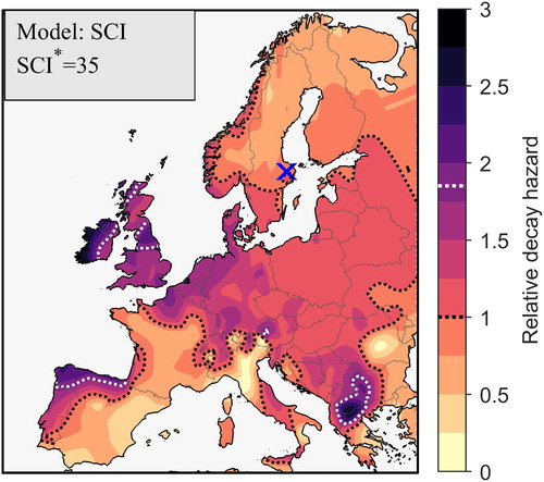
Figure 8 shows the regional variation of the SCI relative to the reference climate. The SCI varies by a factor of 0.5-2.0 with only a select few regions exceeding a relative decay hazard of 2.0, including the north-western coastline of Spain, the west coast of Ireland and a small region in northern Greece. It should be noted that the absolute SCI can be calculated as the product of the relative value and the reference value, SCI${}^{\ast }$, which gives a variation of about 17.5–70. The results are consistent with SCI values from the literature for Spain (Fernandez-Golfin, 2016) and Norway (Lisø et al. , 2006).

Figure 8. Decay hazard map based on the Scheffer climate index. The cross marks the reference site where the relative decay hazard is equal to one and the SCI is equal to 35. The dotted lines divide the three zones originally defined by Scheffer (1971): least favourable conditions for decay ($\mathrm{S}\mathrm{C}\mathrm{I}<35$), intermediate conditions ($35\le \mathrm{S}\mathrm{C}\mathrm{I}\le 65$) and conditions most conductive for decay ($\mathrm{S}\mathrm{C}\mathrm{I}>65$).

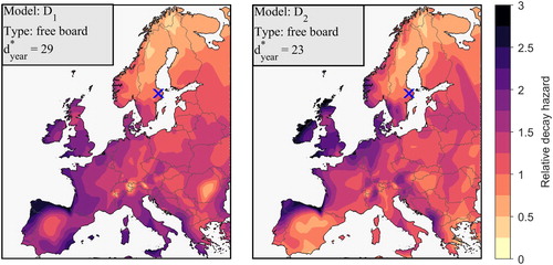
Figure 9 shows the corresponding regional variation of doses, calculated by the two decay hazard definitions for the horizontal board. In general, both maps resemble the SCI with respect to their regional variation and their magnitude in terms of relative decay hazard. There are however distinct regions where the three models differ, most notably along the south and south-west coastlines. These regions are characterized by high relative humidity but relatively low amounts of precipitation. Due to the lack of a lower moisture content threshold, D${}_1$ projects a high risk of decay when the relative humidity is high. In contrast, both the SCI and the D${}_2$ are less dependent on relative humidity but extremely dependent upon precipitation.

Figure 9. Relative decay hazard in Europe based on use-class 3.1 conditions, calculated with modelling approaches ${\mathrm{D}}_1$ (left) and ${\mathrm{D}}_2$ (right), respectively. The cross in each subfigure marks the reference site where the relative decay hazard is equal to one and the annual doses are equal to 29 (left) and 23 (right), respectively.

3.2. Relative performance of the joint

Factor based methods, such as the ones proposed by Meyer-Veltrup et al. (2018) and Wang et al. (2008), rely on the premise that the relative decay rate of different details is more or less independent of the macro climate, so that the effect of detailing can be considered by adjusting the decay rate of a reference member by a design-specific factor, here denoted the relative performance of the detail. The relative performance is then the ratio between the dose of the detail and that of the reference dose.

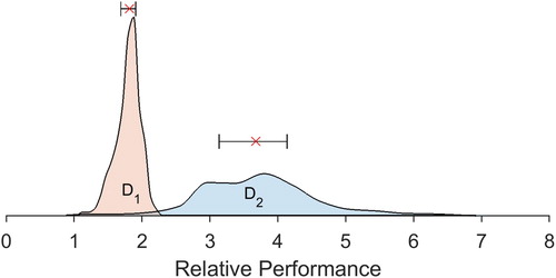
Figure 10 shows the variation of relative performance. The median relative performance calculated from the D${}_1$ and D${}_2$ are 1.8 and 3.7, respectively. This means that the predicted effect of the detail is about two times larger according to D${}_2$ compared to D${}_1$. The results can be compared to the values given in the design guideline by Wang et al. (2008), where the relative increase in decay rate was estimated to be about 2–3 depending on detail type. The variability of the D${}_1$ is relatively low with more than 50% of the values being within the bounds of 1.7 and 2.0. On the contrary, the variability of the D${}_2$ is significant.

Figure 10. Distribution of relative performance. The whiskers extend to the 25th and 75th percentiles and the cross marks the median.

The variability in relative performance is directly associated with the level of accuracy of the factor-based method, as low variability implies that the effect of detailing can be reliably accounted for by adjusting the reference dose by a single detail-specific factor. High variability instead points towards a potential relationship between climate and relative performance.

3.3. Dependency of environmental variables on relative performance

The large variability of D${}_2$, as seen in Figure 10, stems from a dependency between relative dose and annual precipitation, as indicated by their correlation (${\rho }_{\mathrm{X},\mathrm{Y}}$). Out of the three environmental variables, the annual precipitation exhibits the highest correlation to the relative decay rating (${\rho }_{\mathrm{D}2,\mathrm{p}}=-0.7$), with the negative sign indicating that the difference between the free board and the joint diminishes with increasing amounts of precipitation. The dependency on average temperature (${\rho }_{\mathrm{D}2,\mathrm{T}}=-0.3$) and average relative humidity (${\rho }_{\mathrm{D}2,\phi }=-0.4$) were smaller.

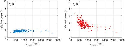
Figure 11 shows how the relative dose varies with annual precipitation, $p_{\mathrm{y}\mathrm{e}\mathrm{a}\mathrm{r}}$. Again, model D${}_2$ predicts a diminishing relative difference between the horizontal board and joint with increasing amounts of precipitation. This effect can be explained by the difference in response on the wood surface when the two details are exposed to cyclic wetting. The surface of the horizontal board dries quickly subsequent to each rain event, so the response in moisture content from individual rain events rarely overlap. Conversely, the surface of the joint is frequently re-wetted before fully recovering from the previous rain event, leading to the total response being less than the sum of two independent responses.

Figure 11. Comparison between relative dose, i.e. the ratio between the dose of the board and the joint, and the annual precipitation, $p_{\mathrm{y}\mathrm{e}\mathrm{a}\mathrm{r}}$, for modelling approaches D${}_1$ and D${}_2$.

3.4. Implications for factor-based methods

The results obtained by the D${}_1$ suggest that it is reasonably accurate to estimate the dose of the joint as the product of the reference dose multiplied by a factor. This is motivated by the linear relationship between the two doses, which implies that the relative difference is approximately constant. The joint studied as part of the present paper gave a factor of approximately 1.7–2.0, which is in agreement with the relative performance of similar joints in the design guideline by Thelandersson et al. (2011), where the relative performance are based on experimental results by Isaksson et al. (2013).

Conversely, D${}_2$ exhibited non-linear effects, where the difference between the joint and the reference board decreased with increasing amounts of precipitation. The results suggest that it would be advantageous to implement a concept of maximum dose, so as to avoid overestimating the decay rate of wood which is permanently damp, where the maximum dose is governed only by the temperature of the site while assuming permanent damp conditions.

3.5. Model uncertainty

Each of the two coupled models is associated with a degree of uncertainty. The numerical model has previously performed well when tested against different wetting sequences in laboratory conditions as well as when tested against outdoor exposure. For simple geometries such as a free horizontal board, the numerical model has proven robust for time-scales up to a few years (Niklewski et al., 2016a). Joints are however more complex as they are governed by multi-directional moisture flow and ambiguous boundary effects. As such, they are generally associated with a higher degree of uncertainty.

The previous data sets used for testing the performance of the numerical model have consisted largely of measurements in the hygroscopic range. For example, the laboratory experiments in question included measuring points not less than 3 mm from the exposed wood surface, where the moisture content rarely exceeded the hygroscopic range. It is plausible that the accuracy is lower in the region near the surface as the moisture conditions are here governed by capillary water movement which is difficult to describe by the simple model employed. As such, the moisture distribution near the exposed surface should be regarded as uncertain and it is reasonable to consider values exceeding the hygroscopic range as being higher than 25%. In this aspect, the simplified logistic model is more robust considering that any values above 25% moisture content correspond to a moisture induced dose of 1. In contrast, the logistic model is less robust as it considers absolute values in the capillary moisture range, which are uncertain.

Decay modelling is generally governed by large uncertainties, both due to lack of available data sets obtained under relevant outdoor conditions and large variability in existing ones. The models are useful for studying relativistic effects, such as relative decay risk, but the absolute values should be considered with some scepticism.

Conclusion and future research

The relative effects of climate and details on the decay hazard were assessed through use of two decay models and two types of wood configuration, including a horizontal board and a joint. In general, the results show how the simulated decay risk varies across Europe, which is basic information needed for assessing the service life of wood as well as for selecting the appropriate level of protection, natural durability and material treatment. While some discrepancies were observed, both decay models were consistent with the features of the well-established SCI, including a similar range of relative decay hazard as well as their regional distribution over Europe. The performance-based model accounts for the material properties and configuration of the wood specimen, while the SCI is based solely on meteorological data. The decay hazard of the joint was, on average, 1.8 or 3.7 times higher than the horizontal board, depending on the decay model employed. One of the models predicted a rather strong relationship between precipitation and the relative effect of the detail, where the relative difference between the board and the joint decreased with increasing precipitation. The other model exhibited no such relationship, and the relative decay hazard could, to some extent, be described as constant and independent of climate.

Future research should focus on verifying the accuracy of the models. This will require a large dataset, preferably with several types of detail configurations and several different climates. The IRG (International Research Group on Wood Protection) durability database is ideal for this purpose (see http://www.irg-wp.com/durability/documents/index.html). Results of this study can be used to select suitable exposure sites for future testing, as test-sites should, ideally, be far apart in terms of decay hazard.

Acknowledgments

J. Niklewski and C. Brischke acknowledge the financial support received from the Wood Wisdom-net project Durable Timber Bridges (DuraTB).

Disclosure statement

No potential conflict of interest was reported by the authors.

Additional information

Funding

E. Frühwald Hansson acknowledges the funding for this work received from the Swedish Research Council Formas (Grant Number: 2012-386 VINNOVA).

References

- Brischke, C., Bayerbach, R. and Rapp, A. O. (2006) Decay-influencing factors: A basis for service life prediction of wood and wood-based products. Wood Material Science and Engineering, 1(3-4), 91–107.
- Brischke, C., Frühwald, E., Kavurmaci, D. and Thelandersson, S. (2011) Decay hazard mapping for Europe. In 42nd Annual Meeting of the International Research Group on Wood Protection (Queenstown, New Zealand, 8-12 May 2011), IRG/WP 11-20463.
- Brischke, C., Meyer, L. and Bornemann, T. (2013) The potential of moisture content measurements for testing the durability of timber products. Wood Science and Technology, 47(4), 869–886.
- Brischke, C. and Meyer-Veltrup, L. (2016) Modelling timber decay caused by brown rot fungi. Materials and Structures, 49(8), 3281–3291.
- Brischke, C. and Rapp, A. O. (2008) Dose–response relationships between wood moisture content, wood temperature and fungal decay determined for 23 European field test sites. Wood Science and Technology, 42(6), 507–1.
- Brischke, C. and Rapp, A. O. (2010) Service life prediction of wooden components – Part 1: Determination of dose-response functions for above ground decay. In 41nd Annual Meeting of the International Research Group on Wood Protection (Biarritz, France, 9-13 May 2010), IRG-WP 10-20439.
- Cornick, S. and Dalgliesh, W. A. (2003) A moisture index to characterize climates for building envelope design. Journal of Thermal Envelope and Building Science, 27(2), 151–178.
- De Meijer, M. and Militz, H. (2000) Moisture transport in coated wood. Part 1: Analysis of sorption rates and moisture content profiles in spruce during liquid water uptake. Holz als Roh-und Werkstoff, 58(5), 354–362.
- Derbyshire, H. and Robson, D. J. (1999) Moisture conditions in coated exterior wood Part 4: Theoretical basis for observed behaviour. a computer modelling study. Holz als Roh- und Werkstoff, 57(2), 105–113.
- EN252 (2015) Field test method for determining the relative protective effectiveness of a wood preservative in ground contact.
- EN335 (2013) Durability of wood and wood-based products – use classes: definition, application to solid wood and wood-based products.
- EN335-1 (2006) Durability of wood and wood-based products – definition of hazard classes of biological attack – part 1: General.
- EN350 (2016) Durability of wood and wood-based products – testing and classification of the durability to biological agents of wood and wood-based materials.
- EN460 (1994) Durability of wood and wood-based products – natural durability of solid wood – guide to the durability requirements for wood to be used in hazard classes.
- Fernandez-Golfin, J., Larrumbide, E., Ruano, A., Galvan, J. and Conde, M. (2016) Wood decay hazard in Spain using the Scheffer index: Proposal for an improvement. European Journal of Wood and Wood Products, 74(4), 591–599.
- Fredriksson, M. and Thygesen, L. G. (2017) The states of water in Norway spruce (Picea abies (L.) Karst.) studied by low-field nuclear magnetic resonance (LFNMR) relaxometry: assignment of free-water populations based on quantitative wood anatomy. Holzforschung, 71(1), 77–90.
- Fredriksson, M., Wadsö, L., Johansson, P. and Ulvcrona, T. (2016) Microclimate and moisture content profile measurements in rain exposed Norway spruce (Picea abies (L.) Karst.) joints. Wood Material Science & Engineering, 11(4), 189–200.
- Isaksson, T., Brischke, C. and Thelandersson, S. (2013) Development of decay performance models for outdoor timber structures. Materials and Structures, 46(7), 1209–1225.
- Isaksson, T. and Thelandersson, S. (2013) Experimental investigation on the effect of detail design on wood moisture content in outdoor above ground applications. Building and Environment, 59, 239–249.
- Koponen, H. (1984) Dependences of moisture diffusion coefficients of wood and wooden panels on moisture content and wood properties. Paperi ja puu, 66(12), 740–745.
- Koponen, H. (1985) Dependence of moisture transfer and diffusion coefficients on temperature. Paperi ja puu, 8, 428–439.
- Lisø, K. R., Olav Hygen, H., Kvande, T. and Vincent Thue, J. (2006) Decay potential in wood structures using climate data. Building Research & Information, 34(6), 546–551.
- Meyer-Veltrup, L., Brischke, C., Niklewski, J. and Frühwald Hansson, E. (2018) Design and performance prediction of timber bridges based on a factorization approach. Wood Material Science & Engineering, 13(3), 167–173.
- Niklewski, J. and Fredriksson, M. (2019) The effects of joints on the moisture behaviour of rain exposed wood: a numerical study with experimental validation. Wood Material Science and Engineering. doi:10.1080/17480272.2019.1600163.
- Niklewski, J., Fredriksson, M. and Isaksson, T. (2016a) Moisture content prediction of rain-exposed wood: Test and evaluation of a simple numerical model for durability applications. Building and Environment, 97, 126–136.
- Niklewski, J., FrühwaldHansson, E., Brischke, C. and Kavurmaci, D. (2016) Development of decay hazard maps based on decay prediction models. In 47nd Annual Meeting of the International Research Group on Wood Protection (Lisbon, Portugal, 15–19 May 2016), IRG/WP 16-20588.
- Niklewski, J., Isaksson, T., Frühwald Hansson, E. and Thelandersson, S. (2017) Moisture conditions of rain-exposed glue-laminated timber members: The effect of different detailing. Wood Material Science & Engineering, 13, 1–12.
- Saito, H., Fukuda, K. and Sawachi, T. (2012) Integration model of hygrothermal analysis with decay process for durability assessment of building envelopes. Building Simulation, 5(4), 315–324.
- Salin, J. G. (2008) Modelling water absorption in wood. Wood Material Science & Engineering, 3(3–4), 102–108.
- Scheffer, T. C. (1971) A climate index for estimating potential for decay in wood structures above ground. Forest Products Journal, 21(10), 25–31.
- Simpson, W. T. (1993) Determination and use of moisture diffusion coefficient to characterize drying of northern red oak (Quercus rubra). Wood Science and Technology, 27(6), 409–420.
- Thelandersson, S., Isaksson, T., Suttie, E., Frühwald, E., Toratti, T., Grüll, G., Viitanen, H. and Jermer, J. (2011) Service life of wood in outdoor above ground applications: Engineering design guideline – background document. Technical report: TVBK-3061. Lund, Sweden, 2011.
- Thelandersson, S. et al. (2017) Durable timber bridges - final report and guidelines. Chapter 2. SP report 2017:25. Skellefteå, 2017.
- Viitanen, H. A. (1997) Modelling the time factor in the development of brown rot decay in pine and spruce sapwood – the effect of critical humidity and temperature conditions. Holzforschung, 51(2), 99–106.
- Viitanen, H., Toratti, T., Makkonen, L., Peuhkuri, R., Ojanen, T., Ruokolainen, L. and Räisänen, J. (2010) Towards modelling of decay risk of wooden materials. European Journal of Wood and Wood Products, 68(3), 303–313.
- Virta, J., Koponen, S. and Absetz, I. (2006) Modelling moisture distribution in wooden cladding board as a result of short-term single-sided water soaking. Building and Environment, 41(11), 1593–1599.
- Wadsö, L. (1993) Surface mass transfer coefficients for wood. Drying Technology, 11(6), 1227–1249.
- Wang, C. H., Leicester, R. and Nguyen, M. (2008) Manual no. 4 – decay above-ground. Forest & Wood Products Australia (FWPA) 2008.