The role of geometry precision in frequency-resonance method for non-destructive wood assessment – numerical case study on sugar maple

ABSTRACT

The application of frequency-resonance method (FRM) for precise log bending testing is limited by complex geometry; usually the cone with variable cross. This case study presents the relationship among non-destructively tested material parameters of sugar maples and the numerical analysis of effect of simplifications in FRM. Four standing stems were measured to find basic geometry parameters, 3D scanned for precise geometry description, tested by pulling test (PT) to obtain elastic parameters, and, finally, cut down to process the logs. Four logs were measured by stress wave propagation (SWP) using an acoustic tomography (AT) device to obtain longitudinal sound velocities and then evaluated by the FRM to obtain natural frequencies in bending and longitudinal vibrations. Comparison was made between the dynamic moduli of elasticity (MOE), calculated from SWP and the FRM, and the static MOE calculated from the PT. In-situ experimental evaluation was accompanied by modal analysis by finite element method (FEM) working at three levels of geometry simplification (beam model, simplified solid model, and scan-based solid model); the natural frequencies of bending and longitudinal mode shapes were analyzed. The influence of geometry precision on the resulting dynamic response of logs was found regarding comparison to the experimental values.

KEYWORDS:

• Non-destructive testing
• sugar maple
• sound propagation
• natural frequency
• finite element method
• modal analysis
• 3D scan
• cross section
• modulus of elasticity

Introduction

Assessment of elastic properties based on the sound wave propagation in wood is a widely used and verified method for material testing (Bucur 1995, Ross et al. 2004). The relationship between sound propagation and the mechanical properties of wood has been examined by Haines et al. (1996), Halabe et al. (1997), Wang et al. (2003), Ross et al. (2004), Bucur (1995), and many others. The most frequently used methods for fully non-destructive wood evaluation are those using the measurement of natural frequency: the resonance method (FRM) and time-of-flight (or stress wave propagation [SWP]) method (Chauhan and Walker 2006, Unterwieser and Schickhofer 2011). The frequency-resonant behavior of wood is affected by many factors, such as wood anisotropy, wood species with macro and microstructure, density, moisture content, temperature, presence of defects, and geometry (Gerhards 1982, Ono and Norimoto 1985, Bucur 1995, Mishiro 1996, Baar et al. 2012). The acoustic wave propagation is directly related to the specific elastic modulus (Hori et al. 2002). Ilic (2003) and Mishiro (1996) concluded that sound wave velocity is not dependent on wood density; Bucur and Chivers (1991) confirm the influence of density (velocity decrease with increasing density). On the other hand, Oliveira and de Sales (2006) described the contradictory density role. The length of axial xylem cells is considered the most significant parameter at the microscopic level (Bucur 1995, Oliveira and de Sales 2006); the microfibril angle in the secondary S2 layer of cell walls plays a crucial role at the ultrastructural level (Ono and Norimoto 1983, Evans and Ilic 2001, Yang and Evans 2003).

The common mode shapes of a vibrating beam are longitudinal, flexural, and torsional. These are the dynamic equivalents of static tension, bending, and torsion. Ravenshorst et al. (2008) used a method based on fundamental frequency for strength grading of tropical hardwoods independent of the species, where the dynamic MOE is strongly correlated with the static MOE and bending strength. Many studies have considered the positive correlations between the dynamic and static MOE; some of these are reported by Liu et al. (2006), who also discovered a significant linear correlation between the static MOE and the dynamic MOE obtained from SWP and the FRM. Mvolo et al. (2021) compared two non-destructive methods (SilviScan and time-of-flight) for lodgepole pine and white spruce, and the relationship between stress wave speed and static MOE was evaluated. Sales et al. (2011) verified the significance of the ultrasonic and transverse vibration techniques for evaluating the static bending MOE as a tool for assessing structural timber pieces. Haines et al. (1996) reported that the mean value of the MOE derived from ultrasonic measurement is about 17% to 22% higher than the static MOE; Wang et al. (2008) observed that the mean values of the ultrasonic-based, dynamic MOE were higher than those of the static MOE by 7.1%, 16.1%, 14.2%, and 9.0% for softwoods. Yang et al. (2002) found that the longitudinal resonance MOE of eucalyptus wood was 39% higher than the static one. Smulski (1991) reported that the dynamic MOE values for maple, birch, ash, and oak were, on average, 22%, 27%, 23%, and 32% higher than the static MOE, respectively.

The FRM provides more information about the material and more reliable results than the SWP method, because the properties (sound velocities, dynamic MOE, etc.) are calculated based on global specimen response at a higher number of waves passing through the material. Based on simplifications of geometry to prismatic beam and assumption of isotropic material, it is frequently used for wood testing, especially for lumber grading, testing of standard samples, or industrial grading sawn-timber in the longitudinal direction, bending, or eventual torsion (Brancheriau and Bailléres 2002, Divos and Tanaka 2005, Brancheriau et al. 2006, Brémaud et al. 2012, Hassan et al. 2013). Zahedi et al. (2021) determined the orthotropic elastic engineering parameters of poplar wood by applying the ultrasonic waves and used them in simulation of mechanical behavior by FEM.

The application for log or standing tree assessment requires a complex approach with respect to multiple parameters (Grabianowski et al. 2006, Legg and Bradley 2016, Lindström et al. 2002, Mora et al. 2009, Wang 2013, Wang et al. 2004, 2007, 2008). Taniwaki et al. (2007) presented the methodology of measuring moisture content of white oak wood based on the measurement of the circumferential vibration mode of a tree, which is independent of the height of a tree. Precise application of FRM for log testing is partially limited by complex geometry; this is usually the cone with variable cross-sections, which is mainly in case used for hardwoods. An evaluation based on testing of bending properties can significantly improve the portfolio of methods for quality assessment of lumber, but this approach requires a more detailed description of geometry. The numerical simulation of the vibration response can be a very powerful tool for observation of predicted behavior, including a range of influencing factors (Dargahi et al. 2020, Liu et al. 2020, Liu et al. 2021). The modal analyses computed by the FEM are, therefore, used as a basic tool for the evaluation of geometry and material effect on frequencies in the paper presented.

Material and methods

Four standing trees of sugar maples (Acer saccharum Marshall) of age approx. 60 years grown at the Davey Tree Expert Company’s Shalersville research station in Ohio, USA (altitude 335 m.a.s.l., average annual total precipitation 810–1000 mm, average annual temperature 8.8–12.2 °C, dusty clay soil) were tested in-situ. Basic tree dendrometry measurements (tree height and cross sections up to 2 m above ground level) were recorded. The stems, up to approximately 2.5 m of height, were scanned by a 3D structure sensor (infrared laser projector module Structure Core by Occipital Inc., with ± 0.29% depth precision, 1280 × 960 depth resolution, and 54 FPS) for a more precise description of the stem geometry. The main dendrometric parameters of measured trees are presented in Table 1.

Table 1. Dendrometric parameters of tested sugar maple trees

	height [m]	diameter at breast height 1.3 [cm]	level of crown bottom [m]	diameter of crown [m]
Tree No. 1 (T1)
direction of puling	14	33.3	2	7
perpendicular direction	15	28.9		10
Tree No. 2 (T2)
direction of puling	17.2	29.8	4	6
perpendicular direction	17.2	30.6		5.5
Tree No. 3 (T3)
direction of puling	15.2	24.3	4	5
perpendicular direction		29.5		6
Tree No. 4 (T4)
direction of puling	19	24.3	4	7
perpendicular direction	20.2	23.8		7

Trees were tested by pulling test (PT), following the procedure described by Vojáčková et al. (2021), to obtain the static force, inclination, and strain response of trees. The PiCUS TreeQinetic system (Argus electronic GmbH) with one forcemeter (resolution 0.01 kN, accuracy 0.3 kN, measuring range 0–40 kN), three elastometers (resolution 0.1 µm, accuracy 1 µm, measuring range +/- 2 mm, distance between measuring points approx. 200 mm), and four inclinometers (resolution 0.002°, accuracy 0.005°, measuring range +/- 15°) was used for PT. Three fully non-destructive loading cycles of up to 0.2° of inclination at tree base were recorded and processed in MATLAB R2021a software to obtain static MOE (Vojáčková et al. 2021).

Trees were cut down and processed into four logs 1.2 m long logs (T1, T2, T3, T4) which were cut out from a scanned part of the trunk (one log per tree). The bottom parts of stems were influenced by the butters-roots and installed devices, therefore the upper parts of the stems were manipulated, resulting in a 1.2 m length pieces with bottom at 60 cm above ground level. Selected logs were without any visible or internal defect (decay), they varied only in outer surface irregularity and shape (see Figure 1). One log (T1) shows a very straight shape, two logs (T2, T3) shows small surface bumps influencing at maximum approx. 6% of cross-section (T2) in 0.3 m of length and 13% of cross-section area (T3) in 0.5 m of length respectively. The T4 log shows small bump (10 cm long) and also the moderate curvature (approx. 4 cm at 1 m length) with the elliptical cross-section at small end (Figure 2).

Figure 1. Laser scan-based geometry models of logs (T1–T4).

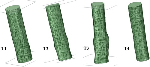
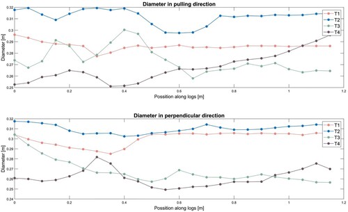
Figure 2. Distribution of diameters along the logs T1–T4.

Within 24 h, four logs were measured by SWP using the acoustic tomography (AT) device PiCUS Sonic Tomograph (Argus electronic GmbH, accuracy of acoustic speed timing 1 µsec). Two spike sensors within 1.2 m were used to obtain sound propagation times in the longitudinal direction. Measurements were taken indirectly by placing sensors on the lateral surface, and directly by placing sensors on the end surfaces of the logs, following methodology described by Hassan et al. (2013). 5 readings in 4 circumference positions for every log piece for both the direct and un-direct method (20 + 20 measurements for every log piece, a total of 160 readings for all pieces and both methods) were performed.

Average times-of-flight were recorded and used for sound propagation velocity and dynamic MOE calculation. At the same time, logs were also assessed by the FRM. The longitudinal and flexural (bending) natural frequencies were recorded and used for sound velocity and dynamic MOE calculation. The longitudinal FRM of a log was induced by striking a hammer (PiCUS Sonic Tomograph, Argus electronic GmbH), on the front. The resulting vibrations were detected by condenser microphone (RODE Lavaloier Go with frequency range 20 Hz–20 kHz, impedance 110 Ohm) placed on the other side. The natural frequency f (Hz) in the longitudinal direction, necessary for the stress-wave speed calculation, was examined by means of fast Fourier transform analysis with use of laptop soundcard (20 real-time readings of frequency for every log piece). The longitudinal dynamic MOE (MOEL) was calculated using the following formula: (1) $MOEL=4\rho f2L2$(1) where ρ is the sample density, f is the frequency of longitudinal vibration, and L is the length of sample.

For the flexure FRM, the points of support were located in the nodes of the fundamental mode of vibration (22% of the log length from each end). The microphone was placed on the lateral side of the log near the middle; the flexural vibration was induced by striking a hammer on the opposite lateral surface in the middle of the length. 20 real-time readings of bending frequency were recorded for every log piece. The frequency of the first bending vibration mode was used for calculating the dynamic bending MOE (MOEB) from the equation: (2) $MO{E}_B=0.947\rho f^2{L}^4{h}^{-2}$(2) where ρ is the sample density, f is the measured frequency, L is the length of the sample, and h is thickness of the sample.

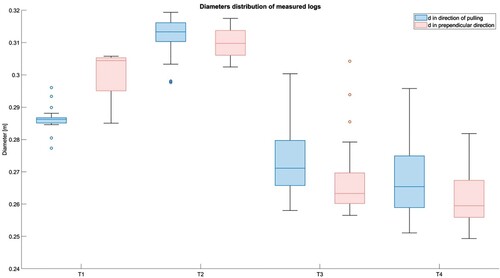
The dynamic MOE, calculated from SWP and the FRM, and the static MOE, calculated from PT, were compared and the relative differences between them were calculated. Density of sugar maple green wood was calculated based on the weights (measured by digital crane loadcell Rock Exotica EnForcer) and volumes (get from 3D finite element model in ANSYS Mechanical APDL software) of logs. In-situ experimental evaluation was accompanied by finite element modal analysis working at three levels of geometry (beam model, simplified solid model, and scan-based solid model). The building of models at different levels of geometry involved the processing of scans. Scanned stems were exported as facets in the obj format for further adjustment in the SpaceClaim package (Ansys® Academic Research Mechanical, Release 2020 R2, ANSYS, Inc.). The processing of scans involved splitting of stems to 1.2 m logs, filling gaps, fixing edges, etc., and the creation of a regular surface mesh before conversion to a solid. The surface mesh was generated into two levels of fineness: 0.02 m element size, and 0.05 m element size, which simulated a different levels of geometry precision obtained from the 3D scans. Surfaces were converted to a solid and imported to ANSYS Mechanical APDL package through connected analyses (Ansys Workbench package). Two levels of finite element mesh (0.03 and 0.05 m edge of elements) were chosen for the coarser scan geometry (0.05 m edge of surface triangulation) to verify the influence of mesh fineness on results. The geometric models (0.02 m surface triangle elements) were made from laser scan by triangulation of point cloud with 0.005 m resolution “from the facets to solid” in Ansys SpaceClaim software are shown in Figure 1. The logs’ geometry differences can be illustrated by the distribution of both log diameters (the first diameter in PT direction and the second in perpendicular) in the length of scan-based solid models of logs (Figure 2) and by the diameters’ variability too (Figure 3). For example, the T3 and T4 samples shows lower diameters (from almost 25 cm) with highest diameter changes (diameter variability) in comparison to T1 and T2; T2 shows the highest diameters (up to 32 cm, locally) and more circular cross-section area; the T1 log have the most elliptical cross-section. T1 can be considered to the straightest, the positions of surface bumps on T2-T4 logs can be identified from Figure 2.

Figure 3. Variability of diameters of logs (T1–T4).

The geometry case of the simplified solid model was built as 1) a cone, 2) a cylinder with a circular cross section, and 3) a cylinder with an elliptical cross section. Also the beam geometry variant with a circular cross section was built for the finite element modal analysis. The diameter used for the definition of the cross section was averaged using perpendicular diameters from each side of the logs. For solid geometry (primitive solids and scans) models, a 10-node tetrahedral element type (SOLID187) was chosen, and for beam models, the choice was a 3-node element (BEAM189). In the case of the solid model, the orthotropic material model was defined.

The properties of wood in different directions were calculated from the longitudinal elastic modulus (EL) and constants for sugar maple (ER 0.132; ET 0.065; GRT 0.02; GTL 0.063; GRL 0.111) according to Kretschmann (2010); similarly, the minor Poisson’s ratios (µTR 0.349; µTL 0.037; µRL 0.065) were used. For beam, the isotropic material model with shear properties was defined; the average constant values of GTL (0.063), GRL (0.111), and major Poisson ratios µLR (0.424) and µLT (0.476) were used. To observe the effect of material properties, these two options were used for the definition of EL: i) the EL was obtained from measured frequency by FRM and calculated longitudinal dynamic MOEL, and ii) the EL was set up to 10.7 GPa (Kretschmann 2010). Wood densities were adapted to each log and geometry model precision level, which imitates the density data acquisition process in-situ. The values for 0.03 m precision level were: 1203 kg/m³(T1), 935 kg/m³ (T2), 918 kg/m³ (T3), 893 kg/m³ (T4); for 0.05 m precision level the 1219, 948, 933 and 908 kg/m³ respectively.

Modal analysis with the block Lanczos algorithm of mode-extraction method within the frequency range of 1–5000 Hz was solved in ANSYS Mechanical APDL solver and 50 modes were extracted. The first bending mode frequency and longitudinal mode frequency were chosen for subsequent validation and analysis of geometry and material influence. Data were compared by relative difference batch calculation processed in MATLAB R2021a.

Results and discussion

Data from PT are represented by three cycles of pulling force (N) recorded by forcemeter versus strain (%), as derived from elongation (mm) recorded by elastometers. The cross-section moduli and bending moments together result in stresses that allow the analysis of MOE from the linear part of the PT records. MOE from PT shows high variability between sensor position (up to 35% difference); generally the most reliable highest position of the elastometer shows the values of static MOE between 4.8 GPa (T2) and 7.7 GPa MPa (T4), which are low in comparison to the literature data (Kretschmann 2010). In addition, the FRM-based dynamic bending moduli ranged from 4.2 GPa (T2) to 5.9 GPa (T1), which is again very low in comparison to the literature data (Kretschmann 2010). These unsatisfactory results of MOE from widespread tree assessment PT method must be subjected to a more detailed analysis in the future.

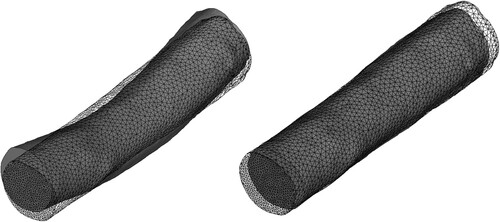
More realistic data are given by the longitudinal FRM, with the average MOE value at 11.4 GPa (20% coefficient variation). With correspondence to the formula (1) working with the length of speciemen the role of log shape irregularities is negligible. The value of FRM based longitudinal MOE is supported by the similar value of average MOE derived from SWP measurements: the average of 11.9 GPa in the case of placing sensors at the end of logs (direct measurement) and about 9% lower values in the case of in-direct measurement from the lateral surface (10.9 GPa on average for T1 to T4 logs). Also, Machado et al. (2009) reported lower values from indirect SWP measurements in comparison to the direct ones. The main results of the numerical modal analyses in ANSYS consist of a) natural frequencies (Hz), b) mode shapes represented by nodal displacements (the sum of X, Y, and Z directions), and c) participation factors in principal directions (X, Y, and Z). Together, these outputs led to individual identification of proper frequencies in all sets of the 50 extracted modes computed for all observed cases of geometry simplification. The typical mode shapes for first bending and longitudinal frequencies are demonstrated in Figure 4 in the case of the scan-based solid model of T1 log. The natural frequency and corresponding mode shape identification (mainly distinction between longitudinal, bending, and torsional modes with defining corresponding frequency range for each mode) can significantly improve the efficiency and interpretation quality of FRM experimental data.

Figure 4. First bending and longitudinal mode shape of log T1.

The beam and simplified solid models provide very clear visual identification of both types of mode shapes and the order corresponding to the typical alternation of orthogonal bending modes, torsion, and longitudinal modes. This was supported by the clear distances of the values of participation factors, which showed an order of magnitude difference in the values in the corresponding directions (higher values of the factors in directions of oscillations of the predominant mass). More complex mode shapes of scan-based models required a detailed individual assessment of longitudinal modes based on nodal displacement plots when the order of mode shape fluctuated from 10 to 18.

For the FMR practice the most important first bending mode frequency and longitudinal mode frequency were chosen for validation and analysis of geometry and material influence. Data comparison is based on the absolute value of average relative differences (errors) within four trees/logs T1–T4.

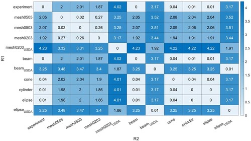
Figures 5 and 6 show the matrices of average absolute relative differences between computed bending frequencies in all cases. In general, the longitudinal modes show lower relative differences between cases (with a maximum at approx. 4.3%) than the bending one (14% maximum). The differences between the models with different mesh density levels are very low (up to 0.5% between the cases for both the longitudinal and bending frequencies). Differences between simplified solid models (cylinder, cone, and cylinder with elliptical cross section) move slightly above 1% for the bending, but very low for the longitudinal vibrations. Very computationally efficient beam models differ more from precise scan-based models (about 10% for bending and 2% for longitudinal) than from simplified solid models (3.3% to 4.4% in bending and up to 0.05% for longitudinal) and have the highest difference in reference to experimental data in bending. Scan-based solid models were the most reliable for bending frequency prediction, but their complexity led to lower reliability for longitudinal frequencies in comparison to more simplified models.

Figure 5. Matrix of average absolute relative differences between bending frequencies of all cases. The relative differences above matrix diagonal use the column (R1) cases as the references; the differences under diagonal use the row (R2) cases as the references.

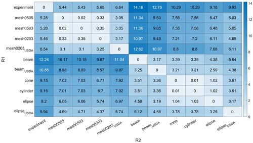
Figure 6. Matrix of average absolute relative differences between longitudinal frequencies of all cases. The relative differences above matrix diagonal use the column (R1) cases as the references; the differences under diagonal use the row (R2) cases as the references.

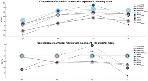
The relative differences between computed and measured bending and longitudinal frequencies of logs (trees T1–T4) are visible from Figure 7. All the simplified models (beam, cylinder, cone, etc.) show the low difference to experiment (and to each other) in longitudinal vibrating. The coincidence and the underestimation can be reported for the scan-based solid models (see Figure 7). The difference between individual, experimentally based material models and the one based on literature is considerable (including both the differences to measured frequencies and differences among the four log cases). Higher relative errors and noticeable differences in frequencies between the numerical models at studied levels of simplification show the sensitivity to the geometry and possibility of precisioning of bending FRM.

Figure 7. Relative differences between computed and measured bending and longitudinal frequencies of logs T1–T4.

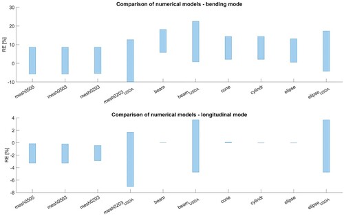
Figure 8 represents the range of relative differences between computed and measured bending and longitudinal frequencies. The beam models and simple-solid models report very low sensitivity to influencing the longitudinal frequencies by transversal variability of geometry (longitudinal frequencies are based on the length of the log) in comparison to complex scan-based models. In general, the bending frequencies among the logs vary more than the longitudinal ones. This may indicate the higher sensitivity of bending modes (mainly, if the complex geometry is incorporated) to changing log parameters in comparison to the one-dimensionally influenced longitudinal modes. Naturally, the general literature-based material model shows higher variability than the material models that correspond to individually derived properties and any precisioning of material parameters can improve the reliability of FRM.

Figure 8. Relative differences between computed and measured bending and longitudinal frequencies; bars show frequency range from T1–T4.

Conclusion

Four sugar maples from the research station served for testing and comparison of experimental methods based on vibro-acoustic principles. They provide mainly the experimental background for validation of numerical models which allows differentiation of numerical modal analyses at ten levels of geometry and material simplification.

An easy and inexpensive in-situ 3D scanning method was successfully deployed to refine the geometry in the FEM modeling process based on the current proprietary simulation package. Beam, simple-solid, and 3D scan-based solid numerical models were compared in the cases of bending and longitudinal vibrations.

Simple solid models report very low sensitivity to influencing the longitudinal frequencies by transversal variability of geometry in comparison to complex, scan-based models. The bending frequencies varied more than the longitudinal ones between log cases, which indicates good sensitivity (and thus good FRM applicability) of bending modes to changing material or geometry parameters. The unified literature-based material model supported the experimental data interpretation but showed higher variability of computed natural frequencies (in average 66% higher range of relative errors) than the material models, which corresponds to individual, experimentally derived properties of each log.

Beam models differ considerably more from precise, scan-based models than from simplified, solid models. Beam models have also the highest difference in reference to experimental data in bending. Scan-based solid models were the most reliable for bending frequency prediction, but vice versa their complexity led to lower reliability for longitudinal frequencies in comparison to more simple solid and beam models. Scan-based models also produced higher amounts of modes and more “difficult-to-read” mode shapes, which required a detailed individual numerical ouputs survey.

Widespread PT on standing trees and the bending FRM on logs reveal variable (up to 35% difference between sensor positions) and relatively low values of elastic constants in comparison with literature data and vibro-acoustic methods. This is motivation to provide more detailed research in this field in the future. The simple, longitudinal FRM applied on logs supplied more reliable results, which were comparable with the low-variable SWP data obtained by AT device measurement in both direct and indirect ways of sensor coupling. SWP direct measurement shows the habitual approx. 10% higher values than the in-direct one.

Acknowledgements

Data that contributed to the presented work were measured during Biomechanical Week 2019 (Ohio, USA) founded by the International Society of Arboriculture and organized by a number of volunteers.

Disclosure statement

No potential conflict of interest was reported by the author(s).

Additional information

Funding

This work was supported by the Ministry of Education Youth and Sports in the Czech Republic [Grant Number #LL1909, ERC CZ].

References

- Baar, J., Tippner, J. and Gryc, V. (2012) The influence of wood density on longitudinal wave velocity determined by the ultrasound method in comparison to the resonance longitudinal method. European Journal of Wood and Wood Products, 70(5), 767–769.
- Brancheriau, L. and Bailléres, H. (2002) Natural vibration analysis of clear wooden beams: A theoretical review. Wood Science and Technology, 36, 347–365.
- Brancheriau, L., Baillères, H., Détienne, P., Kronland, R. and Metzger, B. (2006) Classifying xylophone bar materials by perceptual, signal processing and wood anatomy analysis. Annals of Forest Science, 63, 73–81.
- Brémaud, I., Kaim, E. Y., Guibal, D., Minato, K., Thibaut, B. and Gril, J. (2012) Characterization and categorization of the diversity of viscoelastic vibrational properties between 98 wood types. Annals of Forest Science, 69, 373–386.
- Bucur, V. (1995) Acoustic of Wood (New York: CRC Press).
- Bucur, V. and Chivers, R. C. (1991) Acoustic properties and anisotropy of some Australian wood species. Acoustica, 75, 69–75.
- Chauhan, S. S. and Walker, J. C. F. (2006) Variations in acoustic velocity and density with age, and their interrelationships in radiata pine. Forest Ecology and Management, 229, 388–394.
- Dargahi, M., Newson, T. and Moore, J. R. (2020) A numerical approach to estimate natural frequency of trees with variable properties. Forests, 11(9), 915.
- Divos, F. and Tanaka, T. (2005) Relation between static and dynamic modulus of elasticity of wood. Acta Silvatica & Lignaria Hungarica, 1, 105–110.
- Evans, R. and Ilic, J. (2001) Rapid prediction of wood stiffness from microfibril angle and density. Forest Products Journal, 51, 53–57.
- Gerhards, C. C. (1982) Longitudinal stress waves for lumber stress grading: factors affecting applications: state of the art. Forest Products Journal, 32, 20–25.
- Grabianowski, M., Manley, B. and Walker, J. C. F. (2006) Acoustic measurements on standing trees, logs and green lumber. Wood Science Technology, 40(3), 205–216.
- Haines, D. W., Leban, J. M. and Herbe, C. (1996) Determination of Young's modulus for spruce, fir and isotropic materials by the resonance flexure method with comparisons to static flexure and other dynamic methods. Wood Science and Technology, 30(4), 253–265.
- Halabe, U. B., Bidigalu, G. M., GangaRao, H. V. S. and Ross, R. J. (1997) Nondestructive evaluation of green wood using stress wave and transverse vibration techniques. Materials Evaluation, 55(9), 1013–1018.
- Hassan, K. T. S., Horáček, P. and Tippner, J. (2013) Evaluation of stiffness and strength of Scots pine wood using resonance frequency and ultrasonic techniques. Bioresources, 8(2), 1634–1645.
- Hori, R., Müller, M., Watanabe, U., Lichtenegger, H. C., Fratzl, P. and Sugiyama, J. (2002) The importance of seasonal differences in the cellulose microfibril angle in softwoods in determining acoustic properties. Journal of Materials Science, 37, 4279–4284.
- Ilic, J. (2003) Dynamic MOE of 55 species using small wood beams. Holz als Roh- und Werkstoff, 61, 167–172.
- Kretschmann, D. E. (2010) Mechanical properties of wood. In R. J. Ross (ed.) Centennial ed. Wood Handbook: Wood as an Engineering Material (Madison, WI: General technical report FPL; GTR-190. U.S. Dept. of Agriculture, Forest Service, Forest Products Laboratory), pp. 5.1–5.46.
- Legg, M. and Bradley, S. (2016) Measurement of stiffness of standing trees and felled logs using acoustics: A review. The Journal of Acoustical Society of America, 139(2), 588–604.
- Lindström, H., Harris, P. and Nakada, R. (2002) Methods for measuring stiffness of young trees. Holz als Roh- und Werkstoff, 60, 165–174.
- Liu, Z., Liu, Y., Yu, H. and Juan, J. (2006) Measurement of the dynamic modulus of elasticity of wood panels. Frontiers of Forestry in China, 1(4), 245–430.
- Liu, F., Wang, X., Zhang, H., Jiang, F., Yu, W., Liang, S., Fu, F. and Ross, R. J. (2020) Acoustic wave propagation in standing trees – part 1. numerical simulation. Wood and Fiber Science, 52(1), 53–72.
- Liu, F., Zhang, H., Wang, X., Jiang, F., Yu, W. and Ross, R. J. (2021) Acoustic wave propagation in standing trees – part II. effects of tree diameter and juvenile wood. Wood and Fiber Science, 53(2), 95–108.
- Machado, J., Palma, P. and Simões, S. (2009) Ultrasonic indirect method for evaluating clear wood strength and stiffness. Proceedings of the 7th International Symposium on Non-Destructive Testing in Civil Engineering, 969–974.
- Mishiro, A. (1996) Effect of density on ultrasound velocity in wood. Mokuzai Gakkaishi, 42, 887–894.
- Mora, C. R., Schimleck, L. R., Isik, F., Mahon, J. M., Clark, A. and Daniels, R. F. (2009) Relationship between acoustic variables and different measures of stiffness in standing Pinus taeda trees. Canadian Journal of Research, 39(8), 1421–1429.
- Mvolo, C. S., Stewart, J. D. and Koubaa, A. (2021) Comparison between static modulus of elasticity, non-destructive testing moduli of elasticity and stress-wave speed in white spruce and lodgepole pine wood. Wood Material Science & Engineering, 1–11.
- Oliveira, F. G. R. and de Sales, A. (2006) Relationship between density and ultrasound velocity in Brazilian tropical woods. Bioresource Technology, 97, 2443–2446.
- Ono, T. and Norimoto, M. (1983) Study on Young’s modulus and internal friction of wood in relation to the evaluation of wood for musical instruments. Japanese Journal of Applied Physics, 22, 611–614.
- Ono, T. and Norimoto, M. (1985) Anisotropy of dynamic Young’s modulus and internal friction in wood. Japanese Journal of Applied Physics, 24, 960–964.
- Ravenshorst, G. J. P., van de Kuilen, J. W. G., Brunetti, M. and Crivellaro, A. (2008) Species independent machine stress grading of hardwoods. Proceedings 10th world conference timber engineering (pp. 158–165).
- Ross, J. R., Brashaw, K. B., Wang, X., White, H. R. and Pellerin, F. R. (2004) Wood and timber condition assessment manual. Forest Products Society, Madison, 93 p.
- Sales, A., Candian, M. and Cardin, V. S. (2011) Evaluation of the mechanical properties of Brazilian lumber (Goupia Glabra) by nondestructive techniques. Construction and Building Materials, 25(3), 1450–1454.
- Smulski, S. J. (1991) Relationship of stress wave-and static bending determined properties of four northeastern hardwoods. Wood and Fiber Science, 23(1), 44–57.
- Taniwaki, M., Akimoto, H., Hanada, T., Tohro, M. and Sakurai, N. (2007) Improved methodology of measuring moisture content of wood by a vibrational technique. Wood Material Science & Engineering, 2(2), 77–82.
- Unterwieser, H. and Schickhofer, G. (2011) Influence of moisture content of wood sound velocity and dynamic MOE of natural frequency and ultrasound runtime measurement. European Journal of Wood Products, 69(2), 171–181.
- Vojáčková, B., Tippner, J., Horáček, P., Sebera, V., Praus, L., Mařík, R. and Brabec, M. (2021) The effect of stem and root-plate defects on the tree response during static loading - numerical analysis. Urban Forestry & Urban Greening, 59, 127002.
- Wang, S. Y., Lin, C. J. and Chiu, C. M. (2003) The adjusted dynamic modulus of elasticity above the fiber saturation point in taiwanian plantation wood by ultrasonic-wave measurement. Holzforschung, 57(5), 574–552.
- Wang, X., Ross, R. J., Brashaw, B. K., Punches, J., Erickson, J. R., Forsman, J. W. and Pellerin, R. (2004) Diameter effect on stress-wave evaluation of modulus of elasticity of logs. Wood and Fiber Science, 36(3), 368–377.
- Wang, X., Ross, R. J. and Carter, P. (2007) Acoustic evaluation of wood quality in standing trees. Part I. Acoustic Wave Behavior. Wood and Fiber Science, 39(1), 28–38.
- Wang, S. Y., Chen, J. H., Tsai, M. J., Lin, C. J. and Yang, T. H. (2008) Grading of softwood lumber using nondestructive techniques. Journal of Materials Processing Technology, 208(1–3), 149–158.
- Wang, X. (2013) Acoustic measurements on trees and logs: A review and analysis. Wood Science and Technology, 47(5), 965–997.
- Yang, J. L. and Evans, R. (2003) Prediction of MOE of eucalypt wood from microfibril angle and density. Holz als Roh- und Werkstoff, 61, 449–452.
- Yang, J. L., Ilic, J. and Wardlaw, T. (2002) Relationships between static and dynamic modulus of elasticity for a mixture of clear and decayed eucalypt wood. Australian Forestry, 66(3), 193–196.
- Zahedi, M., Najafi, S. K., Füssl, J. and Elyasi, M. (2021) Determining elastic constants of poplar wood (Populus deltoides) by ultrasonic waves and its application in the finite element analysis. Wood Material Science & Engineering, 1–11.