Determination of a mass-transfer coefficient for wood drying by means of thermography

ABSTRACT

In the present work, it was demonstrated that mass transfer and mass transfer coefficients related to the wood drying process can be satisfactorily quantified using thermography. The method was based on continuous measurements of the wood’s surface temperature, which were converted to a vapor pressure at the wood surface. The results showed that the values of the experimentally obtained transfer coefficients were in the same order of magnitude as values obtained with classical empirical correlations that apply in boundary layer theory. The measurements also showed that an average value of the mass transfer coefficient obtained during drying satisfactorily describes the complete process. The measurement set-up makes it possible to determine a surface potential accurately and continuously, which is useful in the assessment of wood drying processes.

KEYWORDS:

• Thermal imaging
• wood drying
• wood
• spruce
• mass transfer

Nomenclature, units and index

Temperature (°C)	=	$T$
Surface (m2)	=	$S$
Mass transfer coefficient (kg/m2 s Pa)	=	$k_p$
Pressure (Pa)	=	$P$
Time (s)	=	$t$
Characteristic length (m)	=	$x$
Mass of wood sample (kg)	=	$m$
Molar mass (kg/mol)	=	$M$
Moisture flux (kg/m2 s)	=	$\dot{m}$
Atmospheric pressure (Pa)	=	$P_0$
Any relevant moisture potential	=	$X$
Mass transfer coefficient related to $X$	=	$K$
Moisture flux	=	$F$
Thermal conductivity (W/m K)	=	$\lambda$
Air kinematic viscosity (m2/s)	=	$\nu$
Specific heat capacity (J/kg K)	=	$c_p$
Heat transfer coefficient (W/m2 K)	=	$\alpha$
Dynamic viscosity (Pa s)	=	$\mu$
Nusselts number	=	$N{u}_x$
Reynolds number	=	$Re$
Prandtls number	=	$Pr$
Velocity (m/s)	=	$u$

Index
air	=	$a$
wet bulb	=	$w$
vapour	=	$v$
saturation	=	$sat$
Surface	=	$s$

Introduction

In its simplest form, conventional wood drying can be described as an external process where wet wood releases moisture to a surrounding air stream by evaporation from the board surface. During the process, however, three separate drying phases associated with the internal moisture transport can be distinguished: a capillary phase characterized by a continuous supply of water through the internal liquid transport system to the wood surface; a subsequent transition phase where the internal capillary transport system starts to break up and successively limits the free water supply to the surface; and a final diffusion phase characterized by a strongly limited water supply to the surface. The decreasing internal supply of moisture to the wooden surface is thus a major factor affecting the overall, external moisture release.

It is usually assumed that the overall drying rate is proportional to some moisture related potential difference, $\mathrm{\Delta }X$, between the surface of the material, $X_S$, and the air stream, $X_a$: (1) $\begin{array}{c}F=K\mathrm{\Delta }X=K\left(X_S-X_a\right)\end{array}$(1) where $F$ is the moisture transfer between the drying lumber and the air stream and $K$ is a coefficient mainly associated with the external mass transfer. The description is applicable in many situations and fundamentally very simple, but in wood drying, problems with such a description have been reported. Tremblay et al. (2000) pointed out the difficulty of describing the complete drying process with equation (1) since both the external and internal resistances to moisture transport have to be considered. Also Wadsö (1993) and Siau and Avramidis (1996) highlighted difficulties such as applying an appropriate potential in equation (1), especially during the later phases of drying, and to obtain representative values of the transfer coefficients over the complete moisture content range.

Through the years, various potentials $X$ in equation (1) have been considered. In a historical (Dalton 1803) and theoretical perspective (Wadsö 1993, Salin 2010), vapor pressure appears to be an appropriate quantity that explains the evaporation from a wet surface. Other driving forces based on the drying air humidity, such as vapor content (kg H₂O/m³ air) and vapor density (kg H₂O/kg dry air) are also in line with theory and easily determined in a free air stream (Siau and Avramidis 1996). However, since difficulties arise when the conditions at the surface (i.e. the boundary layer) must be determined, other potentials, based on quantities that include the material’s surface moisture content, such as volume or mass based moisture content has been suggested (Ananias et al. 2009). Unfortunately, also such handling of the driving force is problematic, primarily from a theoretical standpoint, since the moisture transport from a drying surface is mainly associated with the properties of the drying gas and the interface, and not the internal properties of the drying product such as moisture content (Söderström and Salin 1993). Also practical issues occur when trying to obtain the surface moisture, as for example by measuring the moisture content in thin layers of veneer (Tremblay et al. 2000) since moisture content is by definition a spatial measure. In some cases, the complicated situation at the surface was handled by assuming thermodynamic equilibrium between the surface moisture content and the surrounding air humidity. Such an assumption in an ongoing drying process may also be questioned, as Rosenkilde and Glover (2002) did when showing that the moisture content close to the surface was almost in equilibrium with the surrounding air during the later stages of drying.

A well-established approach to determine the mass transfer and its related transfer coefficient in various applications is through classical relationships from boundary layer theory, and the analogy between heat and mass transfer. The analogy suggests that convective heat and mass transport, such as in drying, can be seen as, basically, the same phenomenon and therefore could be derived or approximated from each other. However, from several studies, summarized by Söderström and Salin (1993), Wadsö (1993), Siau and Avramidis (1996) and Tremblay et al. (2000), the experimentally obtained values of the transfer coefficients related to wood drying were found to be only a fraction (a tenth or even less) of the values obtained with the classical equations and the analogy, which resulted in the questioning of the applicability of the transfer principles in these contexts. In several works, small values of the mass transfer coefficient were in general obtained at low moisture contents. Although some of these deviations were corrected years before, by introducing different types of correction factors (Kawai et al. 1978), and transfer coefficients dependent on surface moisture content (Plumb et al. 1985, Gong 1992) the origin of these corrections was not thoroughly explained.

In order to clarify the difference between the classical and experimentally determined transfer coefficients Söderström and Salin (1993) suggested a theoretical explanation and argued that the case with constant transfer coefficients has not yet been properly analyzed. Later on, Salin (2010) also showed that a probable reason for the deviations could be an overlooked hysteresis effect. Explanations were also presented by Siau and Avramidis (1996) who reasoned that the experimental values tend to increase for increasing moisture contents and seem to reach close to the classical values for moisture contents around 100% or more. They speculated that the low values of the transfer coefficients measured in the hygroscopic region were a consequence of a decreased area fraction of moist surface. However, when Morén (1992) investigated wood surfaces with thermography no dry spots, at least on a macroscopic scale were observed.

Some experimental studies, of samples of mainly high moisture content show good agreement with results predicted from relationships in the literature (Milota 1994, Tremblay et al. 2000). In these reports, it was nevertheless pointed out that difficulties occurred if trying to investigate partially wet wood surfaces (Milota 1994) and that the transfer coefficient decreases with decreasing moisture content (below ca 80%) (Tremblay et al. 2000).

An observation is that the deviation between experimentally and theoretically determined mass transfer coefficients in wood drying has in most literature been explained on the basis of theory rather than method. Wadsö (1993) is an exception; showing that the low mass transfer rates might partly be due to the experimental methods used being sensitive to various types of disturbances. The theoretical approach to explaining the discrepancy is somewhat surprising, as measuring the surface potential $X_S$ is often pointed out as a main difficulty (Milota 1994, Tremblay et al. 2000). Over the last ten (or twenty) years, the challenge to accurately determine mass transfer coefficients in wood drying has been only sparsely discussed in the scientific literature (the author’s opinion), meaning that the uncertainties with transfer mechanisms and driving forces remain. Probably, this affects not only the possibility for detailed modeling of the wood drying process, but also as Salin (2010) reasoned, the development of accurate simulation and control tools for industrial use.

The present work has its origin in the aforementioned issues. The problem of the difficult-to-determine surface potential during drying was handled experimentally, by surface temperature measurement with thermography in combination with reference surfaces. The objective was to (1) show how the mass transfer coefficient for wood during drying can be determined with the help of thermographic surface temperature measurement; (2) show how process related parameters affect the mass transfer coefficient; and (3) compare the experimentally obtained mass transfer coefficients with calculations based on equations in the heat and mass transfer analogy.

Materials and methods

A laboratory-scale dryer with dry-bulb and wet-bulb temperature control was used for the experimental determination of the mass transfer coefficient.

Board samples of different dimensions of Norway spruce (Picea abies) sapwood with origin from southern Sweden were stored in plastic bags in a freezer until use. Before drying, the samples were thawed in water at a temperature close to the experiment wet-bulb temperature and the end-grain surfaces were sealed with silicone. One sample at a time, placed with the edge and face towards the thermal camera, was dried at a constant drying climate (Figure 1).

Figure 1. Measurement arrangement.

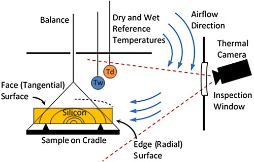
The wood samples were continuously weighed during drying so that the mass loss $\mathrm{\Delta }m$ over time $\mathrm{\Delta }t$, i.e. the rate of evaporation, could be determined. The wood surface temperature $T_s$ was determined with a thermal camera through an inspection window mounted on the dryer door. Reference surfaces at the wet and dry bulb temperatures were also in the field of view of the camera and used to calibrate the temperatures in each image to the actual temperatures at the time of imaging. The total surface area $S$ for evaporation was given by the total sample surface area excluding the two sealed end surfaces, measured in oven-dry state.

The drying trials were interrupted when the weight loss was considered negligible, i.e. when the sample was near the equilibrium moisture content. The airflow velocity was measured with a hot wire anemometer with integrated temperature sensor in nine evenly distributed points in the section for the position of the wood sample. The trial air velocity was determined as the arithmetic mean from the nine measured points. A more thorough description of the experimental set-up and measurement method is found in Lerman et al. (2022).

Calculation of the mass transfer coefficient using the general form of moisture transfer through a boundary layer

The drying rate $\dot{m}$ obtained during the experiments was determined as: (2) $\dot{m}={\displaystyle \frac{\mathrm{\Delta }m}{\mathrm{\Delta }tS}}$(2)

The drying rate may also be expressed with the general form used in equation (1) by substituting the moisture transfer $F$ with $\dot{m}$, $K$ with the mass transfer coefficient $k_p$ and $\mathrm{\Delta }X$ with a moisture related potential such as vapor pressure $\mathrm{\Delta }{P}_v$. The substitution yields: (3) ${\displaystyle \frac{\mathrm{\Delta }m}{\mathrm{\Delta }tS}=k_p\left(P_{v,s}-P_{v,a}\right)}$(3) Here, the vapor pressure at the evaporative interface is $P_{v,s}$ and in the bulk air stream it is $P_{v,a}$. The vapor pressure in the humid air flow is related to the temperature as shown by Carrier (1911) or as here, reformulated by Carpenter (1982) to: (4) $P_{v,a}=P_{sat,w}-{\displaystyle \frac{\left(P_0-P_{sat,w}\right)\left(T_a-T_w\right)}{1546-1.44T_w}}$(4) Here, $P_0$ is the total pressure, $T_a$ the drying air temperature and $T_w$ the wet-bulb temperature. $P_{sat,w}$ is the saturation vapor pressure at the wet-bulb temperature of the air which was calculated with Tetens equations (Murray 1967) as: (5) $P_{sat,w}=610.78e^{{\displaystyle \frac{17.27T_w}{237.3+T_w}}}$(5)

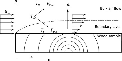
For the vapor pressure in the boundary layer, $P_{v,s}$, an equivalent reasoning as for the air stream was used. As illustrated in Figure 2, the boundary layer temperature is approximated by the measured wood surface temperature. The wet-bulb temperature in the boundary layer is assumed to equal the bulk air wet-bulb temperature since this is the lowest temperature that the wood sample or the surrounding air can acquire by evaporative cooling. The vapor pressure in the boundary layer can thus be formulated as: (6) $P_{v,s}=P_{sat,w}-{\displaystyle \frac{\left(P_0-P_{sat,w}\right)\left(T_s-T_w\right)}{1546-1.44T_w}}$(6) The total moisture transport expressed as a partial vapor pressure potential from the wet surface to the surrounding air is thus expressed by equations (3), (4) and (6) as: (7) $\begin{array}{rl}& {\displaystyle \frac{\mathrm{\Delta }m}{\mathrm{\Delta }tS}=k_p\left(\left(P_{sat,w}-{\displaystyle \frac{\left(P_0-P_{sat,w}\right)\left(T_s-T_w\right)}{1546-1.44T_w}}\right)-\left(P_{sat,w}-{\displaystyle \frac{\left(P_0-P_{sat,w}\right)\left(T_a-T_w\right)}{1546-1.44T_w}}\right)\right)}\end{array}$(7) which after simplification yields: (8) ${\displaystyle \frac{\mathrm{\Delta }m}{\mathrm{\Delta }tS}=k_p{\displaystyle \frac{\left(P_0-P_{sat,w}\right)}{1546-1.44T_w}\left(T_a-T_s\right)}}$(8)

Figure 2. Illustration of a wood sample, air flow and the formation of a boundary layer.

Solving (8) for $k_P$ yields the mass transfer coefficient for every time interval $\mathrm{\Delta }t$: (9) $k_p={\displaystyle \frac{{\displaystyle \frac{\mathrm{\Delta }m}{\mathrm{\Delta }tS}}}{{\displaystyle \frac{\left(P_0-P_{sat,w}\right)}{1546-1.44T_w}\left(T_a-T_s\right)}}}$(9)

In each trial, $k_p$ was determined for a number of $n$ adjacent drying intervals distributed along the complete drying cycle. By adjusting the time interval so that larger $\mathrm{\Delta }t$ was used at low drying rates and vice versa, the influence of mass loss measurement errors was reduced. Each individual trial resulted in between 20 and 100 specific values of $k_p$ obtained throughout the full moisture content range. A mass transfer coefficient $\overline{k_p}$ representing each trial was calculated as the arithmetic mean of $k_p$ from each interval $i$ as: (10) $\overline{k_p}=\sum _{i=1}^n{\displaystyle \frac{k_{p_i}}{n}}$(10)

Calculation of the mass transfer coefficient using the analogy between heat and mass transfer

The heat and mass transfer between the wood samples and the surrounding drying air (Figure 2) is here described by the existence of a thin boundary layer between the sample and the bulk flow where the main temperature and mass concentration gradient develops (Incropera and Dewitt 1996). By the close analogy between these phenomena, the mass transfer coefficient $k_p$ was approximated from the heat transfer coefficient $\alpha$ according to: (11) $k_p={\displaystyle \frac{M_v}{M_a}{\displaystyle \frac{\alpha }{P_0{c}_p}}}$(11) Here, $M$ is the molar mass of water vapor ($v$) and air ($a$), $P_0$ is the pressure and $c_p$ is the specific heat capacity of the humid air. The heat transfer coefficient $\alpha$ depends on the air flow conditions and fluid properties, as well as the geometry and surface roughness of the body and can be calculated from a dimensionless relationship for Nusselt’s number $N{u}_x$ as: (12) $N{u}_x={\displaystyle \frac{\alpha x}{\lambda }}$(12) where $\lambda$ is the thermal conductivity of the medium and $x$ is a characteristic distance in the flow direction. In the literature, a vast number of correlations and numerical expressions of Nusselt’s number is given for different flow conditions, fluid properties and geometries. For board samples, the classical relations given for laminar (13) and turbulent flow (14) over a plate have been used (Siau and Avramidis 1996) and were also used in this work to estimating an average $N{u}_x$: (13) $\overline{N{u}_x}=0.664R{e}^{1/2}P{r}^{1/3}$(13) (14) $\overline{N{u}_x}=0.036R{e}^{4/5}P{r}^{1/3}$(14) where $Re$ and $Pr$ are the Reynolds and Prandtls numbers respectively. The transition between laminar and turbulent bulk flow over the plate depends on the flow conditions and can vary greatly between $Re$ = 10⁵ and $Re$ =  3·10⁶ (McCabe et al. 2001). Usually, and also in this work, the transition value was selected to $Re$ = 5·10⁵ (Incropera and Dewitt 1996).

The Reynolds number for flow over a plate were calculated by the equation: (15) $R{e}_x={\displaystyle \frac{u_{a}x}{\nu }}$(15) where $u_a$ is the fluid velocity, $x$ is the length of the sample in the direction of the flow and $\nu$ is the kinematic viscosity of the air.

The Prandtl number for air was calculated as: (16) $Pr={\displaystyle \frac{\mu c_p}{\lambda }}$(16) where $\mu$ is the dynamic viscosity of the medium.

For the classical relationships, $Re$ was based on total board width, which was significantly lower than the turbulence limit, whereby equation (13) was used to calculate the Nusselt number for all trials. The air’s density, dynamic viscosity, specific heat capacity and heat conduction were derived using established relationships and tables at a boundary layer temperature set to the mean of the bulk air temperature and initial wood surface temperature.

Nineteen trials were carried out with different air temperature, air humidity and air flow rates. All samples were green with initial moisture contents exceeding 100%. The oven dry density was between 462 and 569 kg/m³. The thickness of the samples varied between 17.5 and 28 mm. Operating parameters and test data over the completed trials are shown in Table 1.

Table 1. Summary of drying conditions and sample properties.

Trial/sample	$T_a$ (°C)	$T_W$ (°C)	Air flow rate (m/s)	Dimension in dry state (mm)			Oven dry density (kg/m^3)	Moisture content %
				Thickness	Width	Length		Initial	Final
1	60	37	2.4	17.5	96.0	102	471	159	9.66
2	60	37	2.4	24.0	95.0	108	505	156	7.21
3	60	37	2.4	28.0	98.0	132	491	149	7.29
4	60	48	2.4	17.5	94.3	101	504	154	11.60
5	60	48	2.4	23.5	95.0	106	522	154	8.30
6	60	48	2.4	27.5	97.5	152	498	152	10.40
7	60	54	2.4	18.0	94.9	142	480	159	15.60
8	60	54	2.4	23.5	95.0	99	487	159	15.00
9	60	54	2.4	27.8	95.0	127	480	159	16.50
10	80	60	1.0	21.4	91.5	199	500	150	9.91
11	80	60	2.4	20.5	90.0	196	487	142	7.47
12	80	60	5.0	19.6	91.2	196	479	152	10.40
13	80	60	7.0	20.3	89.0	195	565	109	10.50
14	80	55	2.4	24.7	143.0	195	545	125	5.10
15	80	55	2.4	24.2	51.3	196	462	150	7.69
16	80	55	2.4	24.0	91.0	196	487	123	5.71
17	80	55	2.4	24.0	145.0	200	482	117	10.20
18	80	60	5.0	20.4	45.0	197	487	153	7.84
19	80	60	7.0	24.7	44.0	196	569	134	7.68

Results and discussion

In Figure 3, it is demonstrated for a single drying trial, the importance of choosing suitable time steps $\mathrm{\Delta }t$ when determining the mass transfer coefficient, $k_p$ with equation (9). It is obvious that the low drying rate, i.e. the slow sample weight loss, in the diffusion phase affected the accuracy of $\mathrm{\Delta }m$ and consequently the accuracy of $k_p$. Above fiber saturation (higher drying rates), these problems were not observed. The procedure of weighing which is very sensitive to airflow also affects the accuracy of the mass change. This example illustrates the difficulty with this (and possibly other) gravimetric method(s) to accurately determining the mass transfer coefficient for relatively dry materials during a drying process. The accuracy of the calculation of $k_p$ was increased by extending the time span $\mathrm{\Delta }t$ between the measurement points in the diffusion phase. For a more in-depth discussion on the gravimetric sampling method used in this work, please refer to Lerman et al. (2022).

Figure 3. The mass transfer coefficient $k_p$, calculated with varying $\mathrm{\Delta }t$ as a function of moisture content in trial 16. In this specific trial $\overline{k_p}$ was calculated to 270·10⁻⁹ kg/m² s Pa.

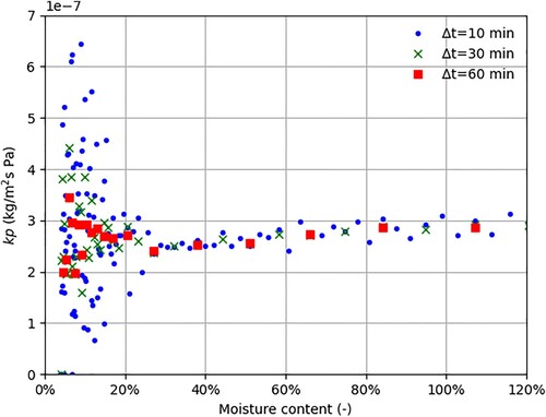
Please note that $k_p$ increases slightly with moisture content for moisture contents above 25% (Figure 3). Using a statistical p-test, we could not reject such a relationship for specific portions of the transition and capillary phases in twelve of the nineteen experiments. The reason is not yet determined but can partially be attributed to systematic deficiencies in the experimental setup. However, the observation is not crucial for the overall context, i.e. that an average value of $k_p$ obtained during the drying experiment ($\overline{k_p}$) adequately describes the process.

Figure 4 summarizes for all trials, the experimental values of the mass transfer coefficient $\overline{k_p}$, obtained with equations (1)–(10) and the corresponding values obtained with the classical relationship for flow over a plate and the analogy, equations (11)–(16). It may be noted that the values of the heat transfer coefficient ranged from 8 to 40 W/m² K which are similar to those reported by e.g. Salin (1997). The drying conditions in the first nine experiments were such that they resulted in similar $\overline{k_p}$. This was in accordance with the corresponding calculations, and is shown as a cluster of overlapping measurement points (Figure 4). It should be noted that there was a strong linear relationship (R² = 0.90) between experimental $\overline{k_p}$ and $k_p$-values obtained with the analogy, which means it is possible to predict the experimental results based on classical relationships.

Figure 4. Comparison of mass transfer coefficients obtained experimentally (y-axis) and by the analogy (x-axis).

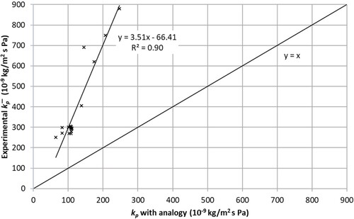
Nevertheless, the lines of best fit in Figure 4 show that the experimentally obtained $\overline{k_p}$ are more than three times higher than those given by the analogy. The findings are reasonable and can be explained by the fact that the classical relationships are based on ideal and steady air flow which normally differs significantly from the flow situation present in small laboratory dryers. The air flow in the laboratory dryer was obviously much more turbulent, which results in higher mass transfer than what the classical equations predict. In addition, the relationships used in the calculations only estimate the transfer from the horizontal surfaces of the sample. Higher values of the Nusselt’s number are expected for surfaces perpendicular to the air flow such as the sample edge side (Salin 1997). Using equation (14) instead of (13) resulted in negligible differences in the calculation of $k_p$ in the studied range.

It has already been discussed why several previous works reported much smaller mass transfer coefficients compared to what the classical equations predict. One suggestion is that a methodology based, rather than theoretical based, explanation should be considered. Moisture content of a drying surface is a discussable concept both in terms of definition and in terms of measurement, so an assumption of a surface potential or a thermodynamic equilibrium based on this quantity may not be appropriate in a context where mass transfer rate is to be quantified. It is reasonable to assume that when vapor pressure based on the surface temperature is used as driving potential for drying, i.e. a measure that the classical equations are based upon, agreement with the analogy is obtained. Previous results were probably reasonable for the potentials and situations that were studied but perhaps not completely comparable with calculations based on the analogy. As Salin (1996) points out, the mass transfer is associated with the gas side and not the properties of the drying product. Of course, sample properties such as shape and surface roughness influence the mass transfer, but primarily by affecting the boundary layer formation.

Based on the linear relationship in Figure 4, a numerical expression for Nusselt’s number reflecting the specific conditions present in the experimental setup could be proposed. Such an expression should be valid for the sample properties, experimental setup and drying conditions used in this work, such as turbulent airflow and a sample moving in the air stream.

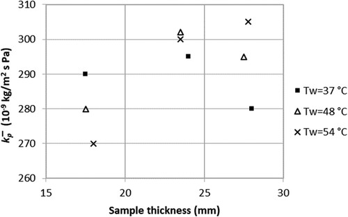
Even if the number of experimental trials in this study was limited, which consequently inhibited an exhaustive analysis of the effect of different variables and the drawing of any definitive conclusions, it is tempting to show how the value of $\overline{k_p}$ changed with some of the studied parameters. Sample thickness and air humidity were varied in the first nine trials (Figure 5). It was expected that the value of $k_p$ increases with sample thickness because the sample surface perpendicular to the air flow then increases and breaks the thermally insulating boundary layer. According to the calculations based on the analogy, a slight increase of $\overline{k_p}$ could also be expected with increased humidity. However, neither sample thickness nor humidity seemed to affect the value of $\overline{k_p}$. The studied thickness range probably too narrow and the influence of humidity too small for an effect to be distinguished with the experimental set-up and given conditions.

Figure 5. The mass transfer coefficient, k_p, as function of sample thickness for different air humidities (trial 1–9).

According to theory, the boundary layer develops in the flow direction along the sample surface and increasingly limits the mass transfer (Figure 2). Therefore, mass transfer coefficients based on the entire sample length are expected to be higher for shorter samples and vice versa. Figure 6 indicates that the narrower samples (∼50 mm) show higher values of $\overline{k_p}$ compared to their wider counterparts. The observed effect is in the same order of magnitude as what the calculations based on the analogy predict.

Figure 6. The mass transfer coefficient, k_p, as function of sample width for different air flow rates (1, 2.4, 5 and 7 m/s).

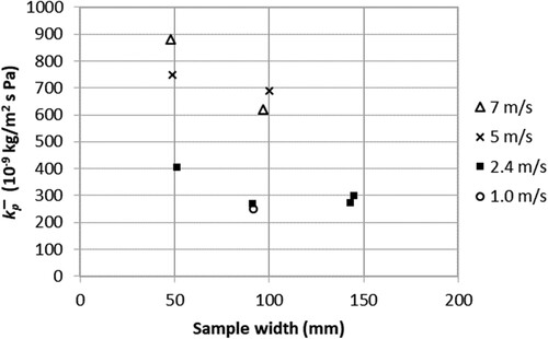
The effect of changed air velocity on $\overline{k_p}$ is also illustrated in Figure 6. Observe that some process parameters slightly differed. For samples with matching widths, $\overline{k_p}$ tends to increase with air velocity. The observation is in line with the theory, which states that the boundary layer thins, and the resistance to mass transfer decreases as the air velocity increases. For a completely wet surface (compare with a free water surface) this implies a successive increase in drying rate with increased air velocity. For lumber, where the free water supply to the surface is limited during most of the drying process, this is only partially true. It is a well-known phenomenon from literature. Wallace and Avramidis (2016) for example stated that when drying the softwood species Hem-fir an air speed of 5 m/s was too high such that it negatively affected the drying rate.

The drying rate and temperature potential between air and surface for different air velocities (trial 10-13) serve to illustrate the phenomenon in more detail (Figure 7). It is worth noting the large difference between the air and surface temperatures, $\mathrm{\Delta }T$ of samples 10 to 12, which were greater than the difference between $T_a$ and $T_w$, indicating that the samples were not in thermodynamic equilibrium with the air at the beginning of the drying process. A non-equilibrium condition is a probable explanation for the initially low drying rates observed. Also, notice the low initial moisture content of sample 13, which also had a high dry density compared to the other samples.

Figure 7. Experimentally determined drying rates (dashed lines) and temperature potentials (solid lines) as function of sample moisture content for different air velocities (trial 10–13).

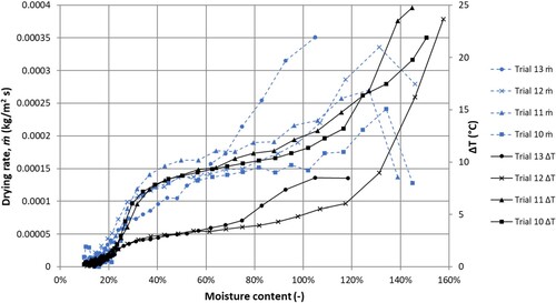
During a large part of the drying process (moisture content < 70%), the drying rate was almost the same for the four trials regardless of air velocity. Recall the large influence of air velocity on $\overline{k_p}$. In Figure 4, the two low velocity trials (10 and 11) are located on the left-hand side, and the two high velocity trials (trial 12 and 13) are the two right points with highest mass transfer coefficient. Only in the capillary regime, when the sample surfaces were wetter, did the samples exposed to higher air velocities show higher drying rates than the low-velocity trials.

The relatively low drying rates for sample 12 and 13, at least during the transition- and diffusion phase, most probably were a consequence of limited internal water supply to the surface, which is revealed by the low temperature potentials. The example and also other studies (Scheepers et al. 2017) show that the surface temperature probably is a representative indicator of the wood material’s surface moisture content and internal transport ability to supply the surface with moisture.

Conclusion

An experimental method for determining the mass transfer coefficient during drying of wood is presented. The method was based on thermographic surface temperature measurements and calculation of the vapor pressure in the boundary layer of the wood surface. With knowledge of the bulk air vapor pressure and the evaporation, the mass transfer coefficient was calculated.

The study showed that the experimentally determined values of the mass transfer coefficient were in the same order of magnitude as what the classical relationships predict, and followed an expected theoretical relationship with the studied process parameters. The complete drying process was described by a mass transfer coefficient associated with the external drying conditions only.

Based on this, it is likely that mass transfer coefficients obtained with the classical equations can be used in wood drying applications if the vapor pressure difference between the wood surface and drying air is used as a drying potential. The method presented thus opens up for the detailed and exhaustive evaluation of the drying process.

It should also be pointed out that the measurement method presented in this and previous work (Lerman et al. 2022) is direct and non-destructive, i.e. the potential difference is measured continuously during drying and without intervention in the process or sample. The work therefore suggests that by knowing the mass transfer coefficient, the rate of evaporation can be determined in real time during drying. In principle, the technique should also be useful on an industrial scale in order to follow, evaluate and possibly control drying processes. An industrial application of the measurement technology is under development.

Disclosure statement

The authors own shares in Hydraterm AB, a startup company that develops non-contact moisture content measuring devices for the sawmilling industry.

Additional information

Funding

This work was supported by Södra Skogsägarnas Stiftelse för Forskning, Utveckling och Utbildning [grant number 2019-136] and Familjen Kamprads Stiftelse [grant numbers 20180286, 20200107].

References

- Ananias, R.A., et al., 2009. Using an overall mass-transfer coefficient for prediction of drying of Chilean coigüe. Wood and Fiber Science, 41 (4), 426–432.
- Carpenter, J.H., 1982. Fundamentals of psychrometrics. Carrier Corp, Syracuse, 57.
- Carrier, W.H., 1911. Rational psychrometric formulae. Transactions of the American Society of Mechanical Engineers, 33, 1005.
- Dalton, J., 1803. Experimental essays on the constitution of mixed gases: on the force of steam or vapour from water and other liquids in different temperatures, both in a Torricellian vacuum and in air; on evaporation and on the expansion of gases by heat. Journal of Natural Philosophy, Chemistry, and the Arts, 6, 257.
- Gong, L., 1992. A theoretical, numerical and experimental study of heat and mass transfer in wood drying. Ph.D. Thesis. Washington State University, Dept. of Mechanical and Material Engineering, U.S.
- Incropera, F.P., and Dewitt, D.B., 1996. Fundamentals of heat and mass transfer. New York: Wiley.
- Kawai, S., Nakato, S., and Sadoh, T., 1978. Prediction of moisture distribution in wood during drying. Mokuzai Gakkaishi, 24, 6.
- Lerman, P., Scheepers, G., and Wiberg, P., 2022. A laboratory setup for measuring the wood-surface temperature during drying by means of thermography. Wood Material Science & Engineering, 18 (2), 701–706. doi:10.1080/17480272.2022.2066479.
- McCabe, W.L., Smith, J.C., and Harriott, P., 2001. Unit operations of chemical engineering. Boston: McGraw Hill.
- Milota, M.R., 1994. Mass transfer coefficients as a function of position in a lumber kiln. Paper presented at the 4th IUFRO Wood Drying Conference, Rotorua, New Zealand.
- Morén, T., 1992. Infrared thermography in the analysis of moisture flux from drying wooden surfaces. Drying Technology, 10 (5), 1219–1230.
- Murray, F.W., 1967. On the computation of saturation vapor pressure. Journal of Applied Meteorology, 6 (1), 203–204. doi:10.1175/1520-0450(1967)006<0203:OTCOSV>2.0.CO;2.
- Plumb, O.A., Spolek, G.A., and Olmstead, B.A., 1985. Heat and mass transfer in wood during drying. International Journal of Heat and Mass Transfer, 28 (9), 1669–1678.
- Rosenkilde, A., and Glover, P., 2002. High resolution measurement of the surface layer moisture content during drying of wood using a novel magnetic resonance imaging technique. Holzforschung, 56 (3), 312–317.
- Salin, J.-G., 1996. Mass transfer from wooden surfaces and internal moisture non-equilibrium. Drying Technology, 14 (10), 2213–2224.
- Salin, J.-G., 1997. Prediction of heat and mass transfer coefficients for individual boards and board surfaces. A review. Paper presented at the 5th International IUFRO wood drying conference, Quebec City, Canada, August 13–17, 1996 (11021071 (ISSN)). Retrieved from http://urn.kb.se/resolve?urn=urn:nbn:se:ri:diva-28675.
- Salin, J.-G., 2010. Problems and solutions in wood drying modelling: History and future. Wood Material Science and Engineering, 5 (2), 123–134.
- Scheepers, G., Wiberg, P., and Johansson, J., 2017. A method to estimate wood surface moisture content during drying. Maderas Ciencia y Tecnología, 19, 133–140. https://scielo.conicyt.cl/scielo.php?script=sci_arttext&pid=S0718-221X2017000200001&nrm=iso.
- Siau, J.F., and Avramidis, S., 1996. The surface emission coefficient of wood. Wood and Fiber Science: Journal of the Society of Wood Science and Technology, 2, 178–185.
- Söderström, O., and Salin, J.-G., 1993. On determination of surface emission factors in wood drying. Holzforschung, 47, 391–397. http://urn.kb.se/resolve?urn=urn:nbn:se:ri:diva-5684.
- Tremblay, C., Cloutier, A., and Fortin, Y., 2000. Experimental determination of the convective heat and mass transfer coefficients for wood drying. Wood Science and Technology, 34 (3), 253–276.
- Wadsö, L., 1993. Surface mass transfer coefficients for wood. Drying Technology, 11 (6), 1227–1249.
- Wallace, J., and Avramidis, S., 2016. Impact of airflow on hem-fir kiln drying. Drying Technology, 34 (11), 1354–1358.