Moisture gradients in sawn timber during aggressive kiln drying investigated with X-ray computed tomography

ABSTRACT

Reducing the time for drying sawn timber to a certain moisture level without deteriorating its quality is increasingly important for an economic and energy-efficient industrial timber-drying process and to support the transition to a sustainable society. It is, however, crucial to ensure that the quality of the timber, i.e. the degree of distortion, cracking, discolouration, and moisture variation within and between the pieces in a drying batch, is not compromised. Drying-simulation software tend to be too conservative in drying-rate recommendations, which has been observed in practise particularly for large cross-section timber of Norway spruce. This study investigated the drying rate and checking occurrence of centre-yielded Norway spruce planks when dried with more aggressive schedules than normally used in practise, i.e. using higher dry-bulb temperatures and/or lower relative humidities than recommended in the conventional optimisation programmes used in the sawmill industry in Sweden. The objective was to investigate the possibility to considerably reduce the total drying time without compromising the quality of the dried timber. The quality of the planks was indirectly assessed by estimating their moisture-content distributions, calculating the moisture gradients and monitoring checking. This was achieved with 4D (3D + time) X-ray computed tomography and a recently developed image processing algorithm based on elastic image registration. The key findings in this study suggest that Norway spruce timber can be dried with significantly higher temperatures and lower relative humidities than suggested by simulations, leading to reduced total drying time without inducing checking. This methodology can help to improve the design of drying schedules to reduce drying time and energy consumption while maintaining timber quality at a level accepted by the customers.

KEYWORDS:

• CT scanning
• elastic image registration
• moisture transport
• sawn-timber quality
• wood

1. Introduction

1.1. Kiln drying, an energy-consuming process

Within the project Energy Efficiency in the Sawmill Industry (EESI 2010-2015), it was demonstrated that the energy used in timber drying in Swedish sawmills is 20% higher than the energy needed to remove the water from the wood (Andersson et al. 2011). Investments in new technologies have reduced the energy consumption in the drying stage, but the drying process is still a high-energy consumer and it has poor energy efficiency (Konopka et al. 2021). The main reason for energy consumption not being significantly reduced could be that the models that control the drying process are not optimised to minimise the drying time or energy consumption, but only to maximise the resulting timber quality. There is a lack of basic knowledge of the process, i.e. of the phenomena that control moisture transport during drying and how this affects stress concentrations in the material that can lead to wood damage, and subsequently quality downgrading. Public data on the total cost of drying damage is not available, but a very low estimate based on experience from sawmill representatives in Sweden is, however, 100 million euros annually. The annual production of sawn timber in the Swedish sawmilling sector is around 19 million m³, which means that drying kilns must evaporate around 7 million tonnes of water with a heat consumption of 6-7 TWh. Based on the energy theoretically needed to remove the water from the wood, only 4 TWh would be necessary, which means that there is a potential to save 2-3 TWh. Such a reduction in energy consumption would allow the release of bioenergy for other purposes and would also result in reduced costs.

1.2. Traditional drying schedules are outdated

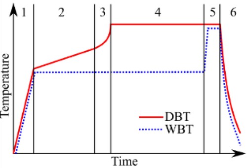
When a green log is sawn, the timber must shortly be dried in a controlled way to avoid distortion, cracking, moulding, and other phenomena that deteriorate its quality. Despite being an energy-intensive process, kiln drying is a standard practice in the industrial production of sawn timber, especially for softwoods, to obtain good quality products in a faster manner than e.g. natural drying in the free air (seasoning). During drying, the average moisture content (MC) is reduced below the FSP, which is approx. 28% for Norway spruce (Picea abies (L.) Karst.) (Wiberg and Morén 1999), to levels according to the final use of the product (approx. 8–18%). Kiln drying also aims to reach a uniform MC both in the batch and within each single piece of sawn timber. Therefore, heated air is blown through the timber packages to take up the water evaporating from the surface of the sawn timber in a controlled fashion and extracted from the kiln through venting. A classic batch-kiln drying schedule consists of six regimes corresponding to different heat and moisture transport modes in the timber, as shown in Figure 1.

Figure 1. The different regimes in a typical drying schedule for Norway spruce sawn timber: (1) heating, (2) capillary regime, (3) transition regime, (4) diffusion regime, (5) conditioning, and (6) cooling. DBT and WBT stand for dry-bulb temperature and wet-bulb temperature, respectively.

The drying schedules used in Swedish sawmills are provided by computer simulation tools based on parameters such as tree species, density, initial MC, wood temperature, heartwood-sapwood proportion, and target MC. Nevertheless, current simulations tools are often conservative in terms of drying rate (Florisson et al. 2022). The drying rate is regulated by estimating the stress value that causes checking based on a one-dimensional model describing moisture diffusion, heat transfer, viscoelastic creep, and mechano-sorption (Salin 1999).

It is sometimes observed within the Swedish sawmilling industry that operators empirically modify the simulated schedules to increase the drying rate and turn them into what will be referred to as aggressive schedules. This is achieved by increasing the DBT, decreasing the WBT, or both. An increase in the DBT has the advantage of thermo-plasticising wood, thermo-hygro-plasticisation refers to the combined effect of temperature and moisture on softening the wood material, consequently decreasing its stiffness (Salmen 1982) which reduces cracking. It also increases the capacity of the air to carry water so that less air needs to be extracted from the kiln to reduce the RH of the air inside. A decrease of the WBT contributes to reducing the energy consumption not only by speeding up the process, but by requiring less thermal energy to reduce the RH of the kiln.

1.3. Moisture gradient as a quality indicator

When implementing aggressive drying, the MG is expected to increase as the MC at the surface of the timber will be lower than in conventional schedules. If the MG between the surface and core is too high, the tensile stresses at the timber surface may exceed the tensile strength of the wood material causing checking (Florisson et al. 2019, Avramidis et al. 2023). As the MG influences both the drying rate and checking of the sawn timber, it was considered as a relevant parameter to monitor in relation to the optimisation of the drying process. It is possible to quantify MG through X-ray CT as a useful parameter to study for the drying process (Poupet et al. 2022). A MG is defined as the difference of MC between two points per unit distance, and often calculated with the slicing method and expressed in percentage (Stevens and Pratt 1961). Typically, one point is chosen at the surface and the other at a certain depth within the timber volume. This method to calculate the MG is in practice simple to perform, but MC measurements by CT scanning allow for a more accurate approach, as it will be shown in the present study.

The MC in wood can reliably be measured gravimetrically, but this method is destructive and it is not possible to follow the spatial MC changes during the drying. Different measuring techniques have been used for measuring the spatial MC variation in wood such as neutron radiography (Lanvermann et al. 2014, Sanabria et al. 2015), low-field nuclear magnetic resonance (Xu et al. 2017), microwave propagation (Aichholzer et al. 2018), near-infrared spectroscopy (Awais et al. 2022), and X-ray CT (Hansson and Fjellner 2013, Couceiro 2019, Florisson et al. 2022). Out of the previously mentioned techniques, macro X-ray CT provides advantages such as short scanning times of full-size sawn timber, safe and relatively uncomplicated use. X-ray CT is used industrially in sawmills for grading round timber and optimisation of the sawing pattern, and in research facilities to assess material properties of wood such as anatomical features and MC (Beaulieu and Dutilleul 2019). The working principle of an X-ray CT scanner is based on an X-ray source and a detector rotating in tandem around an object to reconstruct its tomogram, which consists in a matrix of volume elements (voxels) that encode the beam attenuation as a parameter known as the CT number (Withers et al. 2021). For wood, it has been established that a linear relationship exists between the CT number and the density (Benson-Cooper and Knowles 1982, Mull 1984, Lindgren 1985), although the exact relationship depends on the specific CT scanner used (Freyburger et al. 2009, Wang et al. 2019).

1.4. Image processing

Image processing is required to determine the MC of the wood in a tomogram of interest by comparing it to a reference tomogram of the exact same wood region at a known MC distribution, which is for practical reasons the completely dry state (0% MC). This comparison cannot be performed directly as the voxels between these two states are not aligned due to the inevitable anisotropic shrinkage associated with drying, which deforms the cross section of the timber. Image registration consists of mapping one tomogram to the other, aligning the tomograms, and having a correspondence between the voxels in the same location of both tomograms. Rigid image registration is based on global transformations, which can be linear (translations, scaling, rotations) or affine (also shear) while non-rigid image registration also includes local deformations and are often qualified as elastic (Oliveira and Tavares 2014). Local deformations in wood are best captured using elastic image registration (Patera et al. 2018) and different studies used such technique to investigate MC distributions (Hansson and Fjellner 2013, Riley et al. 2022). Another important stage to estimate the MC distribution is the correction of the density values between the original tomogram and its registered (mapped) equivalent. Correcting registered densities involves estimating local shrinkage or strain, in first approximation as a linear relationship to MC (Watanabe et al. 2008), but more advanced methods use the displacement field information from digital-image correlation (Miettinen, et al. 2016) or image registration (Hansson and Fjellner 2013). Most of the previously mentioned studies work in two-dimensions (2D). In this study, a recently developed four-dimensional (4D) method based on the elastic image registration library Elastix (Klein et al. 2010) will be applied to analyse the MC distribution both in space (3D) and time (Poupet et al. 2023).

The aim of the current study was to investigate the effects of aggressive drying on the development of MG within large cross sections of Norway spruce sawn timber. The purpose is to ultimately optimise industrial drying of sawn timber. An experiment was developed to obtain four-dimensional (4D, space, and time) X-ray computed tomography scans during kiln drying. In this experiment, a traditional schedule from a Swedish sawmill was adjusted to introduce aggressive drying. The image-processing algorithm developed by Poupet et al. (2023) was used to evaluate the MG based on such tomograms.

1.5. Objectives

The current study is driven by the vision of a 20% reduction in energy consumption during timber drying in the Swedish sawmilling industry, in accordance with potential savings reported by Andersson et al. (2011). The aims of the project are to develop an experimental method to study aggressive drying and to use a recently developed image-processing tool that allows for a detailed analysis of MG during drying. The specific objective of this study is to test the following hypotheses: (1) that the MG would increase as the schedule’s aggressivity increases; (2) that schedules that are considerably more aggressive than those proposed by the simulation software will not cause cracking.

2. Materials and methods

The experimental method was designed around a medical X-ray CT scanner with integrated kiln. An industrial drying schedule obtained with a drying simulation software commonly used by Swedish sawmill was modified to create more aggressive drying conditions by raising the DBT and lowering the WBT. In the following subsections, the specimens’ preparation will be discussed, and the experimental setup and image-processing algorithm will be introduced.

2.1. Specimen preparation

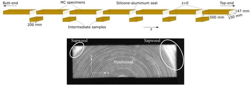
In this study, centre-yielded block-sawn timber, which is well-known prone to checking during drying (Niemz et al. 2023), was investigated. Six centre-yield planks (labelled A to F) of Norway spruce in green state were collected in a local sawmill in the region of Västerbotten, northern Sweden. The logs from which the specimens were sawn all grew in the same forest region. The cross-sectional dimension of the timber was 47 × 150 mm and defect-free specimens with a length 500 mm were sawn, separated by intermediate samples of length 200 mm that were used to obtain gravimetric measurements of MC prior to the experiments. The heartwood of all specimens was present across the whole thickness (Figure 2). For each plank, the specimens were labelled from 1 (closer to the butt-end) to 7 (closer to the top-end). To prevent drying in the longitudinal direction, the specimens were sealed on their cross-sections with a layer of silicone Casco SuperFix + [Sika, Baar, Switzerland], followed by a layer of household aluminium and another layer of silicone. The specimens were sprayed with water, wrapped in plastic film, and stored in frozen condition to limit uncontrolled drying before the start of the experiments.

Figure 2. Preparation of specimens for the experiments (top) and tomogram of specimen A3 at z = 150 mm (bottom).

2.2. Experiment

2.2.1. Experimental setup

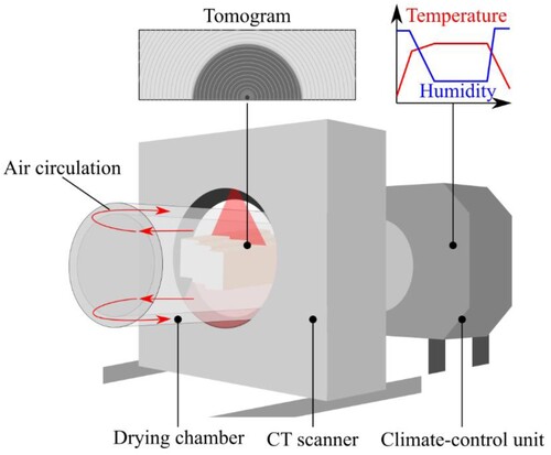
The experimental setup consisted of a Siemens Somatom Emotion Duo CT scanner [Siemens, Munich, Germany] and a custom-made timber-drying kiln consisting of a climate-control unit and drying chamber as shown in Figure 3. In each experimental set-up, six specimens in frozen conditions were placed in the drying kiln with the longitudinal direction parallel with the airflow of the kiln. The climate in the kiln was controlled through heat, steam, ventilation, and air circulation according to the provided schedule. The CT scanner acquired the 3D tomograms of the specimens during the experiment at 1-hour intervals with a voxel size of 0.98 mm × 0.98 mm in the transverse plane (x, y) and 3 mm in the longitudinal direction (z) of the specimens. A bottle containing distilled water was placed in the drying chamber and scanned simultaneously with the specimens as an imaging phantom for intensity calibration of the density values (0 kg/m³ for air, and 1000 kg/m³ for distilled water). The eventual occurrence of checking or other types of cracks in tomograms would be clearly visible and monitored during the drying process.

Figure 3. Experimental setup: the specimens were placed in the drying kiln to be simultaneously CT scanned and dried. The arrows within the drying chamber represent the direction in which the heated and moist air circulates.

2.2.2. Drying schedules

In the first experimental set-up, a schedule generated with the industrial drying-kiln management software Valmatics 4.0 [Valutec, Skellefteå, Sweden] was used. This schedule was considered as the reference schedule (S0) and it was generated using the input parameters presented in Table 1. The mean MC and standard deviation were obtained with the gravimetric measurements performed on the intermediate samples according to the EN 13183-1 standard (Standards Sweden 2004).

Table 1. Input parameters used in the drying simulation software to obtain the reference schedule.

Species	Norway spruce
Cross-sectional dimensions	47 mm × 150 mm
Mean MC	40.4%
MC standard deviation	9.8 percentage points
Log diameter	201.6 mm
Heartwood diameter	165.8 mm
MC sapwood	136.6%
Green density	380 kg/m3
Target MC	18%

The reference schedule was modified to make it more “aggressive”, aiming to find the conditions at which the quality of the sawn timber became unacceptable, which was established to be when the specimens show surface checking. The modified, aggressive drying schedules (S1 to S4) were obtained by decreasing the WBT after the heating regime, which reduced the RH during capillary, transition, and diffusion regimes. Five schedules including the reference were tested, and their respective maximum DBT, minimum WBT, and minimum RH values are shown in Table 2.

Table 2. The drying schedules (S0-S4), with their corresponding max. DBT (dry-bulb temperature), min. WBT (wet-bulb temperature), and min. RH (relative humidity). Schedule S0 is the least aggressive schedule and S4 the most aggressive one.

Schedule id	DBT (°C)	WBT (°C)	RH (%)
S0	74	55	40
S1	74	44	20
S2	74	37	10
S3	84	40	8
S4	94	38	3

For schedules S1 and S2, the WBT was reduced and the DBT profiles were set to be similar to the reference schedule, nevertheless some adjustments were automatically performed by the software: the heating phase was shorter than in S0 and the temperature increase during the capillary regime was slower. It is thus likely that the specimens in schedules S1 and S2 were less thermo-plasticised than the specimens in S0 and more prone to checking. It was not possible to further reduce the RH by only reducing the WBT, thus the DBT was increased for the schedules S3 and S4. No capillary regime was performed in S3 and S4 and instead, the schedule went directly from the heating regime to the diffusion regime to create even more aggressive drying conditions. The heating regimes in S3 and S4 were longer than in the previous schedules, this was not intentional and was the result of an asymptotic behaviour of the DBT and WBT profiles. However, it could be verified that the MG did not increase during prolonged high RH levels as expected. The specimens in schedules S3 and S4 were therefore more thermo-plasticised than in S0, S1, and S2 and consequently less prone to checking. Schedule S0 is considered as the least aggressive schedule and S4 as the most aggressive one.

When each drying set-up was finished, the specimens remained in the chamber to be oven-dried at 103 ± 2°C for 48 h, with the ventilation fully open to extract the evaporated moisture. A CT scan was performed after this period to obtain the oven-dry tomogram of the specimens, i.e. the tomogram corresponding to a MC of 0%.

2.3. Image-processing algorithm

2.3.1. Theory

A registered pixel at spatial coordinates x = (x, y, z) in the Cartesian system is a deformed quadrilateral polygon of area A₀ and density $\rho \left(x\right)$, it is intersected with the reference pixels and each intersection area A_i is computed (Poupet et al. 2023). The corrected densities ${\rho }^{\mathrm{\prime }}\left(x,\mathrm{t}\right)$ are calculated according to: (1) ${\rho }^{\mathrm{\prime }}\left(x,\mathrm{t}\right)=\sum _{\mathrm{i}}{\rho }_{\mathrm{i}}\left(x,\mathrm{t}\right).{\displaystyle \frac{{\mathrm{A}}_{\mathrm{i}}}{{\mathrm{A}}_0}}$(1) The MC distributions are then computed with: (2) $w\left(x,\mathrm{t}\right)={\displaystyle \frac{{\rho }^{\mathrm{\prime }}\left(x,\mathrm{t}\right)-{\rho }_0\left(x\right)}{{\rho }_0\left(x\right)}}$(2) A Gaussian blur of standard deviation (σ) 3 was used to smoothen the MC distributions and eliminate outliers. The MG is defined as a vector field and its orthogonal components are approximated and computed by central differences: (3) $\begin{array}{rl}\mathrm{\nabla }w\left(x,\mathrm{t}\right)& =|\begin{array}{c}{\mathrm{\nabla }}_{\mathrm{x}}w\left(x,\mathrm{t}\right)\\ {\mathrm{\nabla }}_{\mathrm{y}}w\left(x,\mathrm{t}\right)\\ {\mathrm{\nabla }}_{\mathrm{z}}w\left(x,\mathrm{t}\right)\end{array};{\mathrm{\nabla }}_{\mathrm{r}}w\left(x,\mathrm{t}\right)\\ & ={\displaystyle \frac{w\left(x-u_{\mathrm{r}},\mathrm{t}\right)-w\left(x+u_{\mathrm{r}},\mathrm{t}\right)}{2\Vert u_{\mathrm{r}}\Vert }}\end{array}$(3) with $u_{\mathrm{r}}$ the unit vector in the Cartesian direction r (x, y, or z). The voxels surrounding the specimens and representing air with a density of 0 kg/m³ were not considered in this computation. This definition of MG is more adapted to the CT data than other definitions often used in wood science such as the one provided by Esping (1988), because MC is considered at each voxel. Moreover, the traditional definition of MG can be retrieved from this new definition as follows: consider two voxels within a wood volume with spatial coordinates $x_1=\left({\mathrm{x}}_1,{\mathrm{y}}_1,{\mathrm{z}}_1\right)$ and $x_2=\left({\mathrm{x}}_2,{\mathrm{y}}_2,{\mathrm{z}}_2\right)$, respectively. In its traditional definition, the MG is expressed as: (4) ${\left({\displaystyle \frac{\mathrm{\Delta }w}{\mathrm{\Delta }x}\left(\mathrm{t}\right)}\right)}_{x_1,x_2}={\displaystyle \frac{\left|w\left(x_1,\mathrm{t}\right)-w\left(x_2,\mathrm{t}\right)\right|}{\mathrm{d}}}$(4) where $\mathrm{d}=\sqrt{{\left({\mathrm{x}}_1-{\mathrm{x}}_2\right)}^2+{\left({\mathrm{y}}_1-{\mathrm{y}}_2\right)}^2+{\left({\mathrm{z}}_1-{\mathrm{z}}_2\right)}^2}$ the Euclidean distance between $x_1$ and $x_2$. The gradient theorem can be applied in a discrete form to express the MG between two voxels as a sum of MG: (5) ${\left({\displaystyle \frac{\mathrm{\Delta }w}{\mathrm{\Delta }x}\left(\mathrm{t}\right)}\right)}_{x_1,x_2}=\sum _{x_1}^{x_2}\mathrm{\nabla }w\left(x,t\right).u_{\mathrm{r}}$(5) Equation (5) is valid independently of the path taken to join the points $x_1$ and $x_2$ as it is a property of conservative vector fields. In the chosen coordinate system, the vertical component of the MG, i.e. ${\mathrm{\nabla }}_{\mathrm{y}}w\left(x,\mathrm{t}\right)$will correlate to the tangential stresses, thus the checking. Moreover, it was statistically observed within each specimen across the different schedules that the inequality presented in Equation (6) holds: (6) $\Vert {\mathrm{\nabla }}_{\mathrm{z}}w\left(x,\mathrm{t}\right)\Vert \le \Vert {\mathrm{\nabla }}_{\mathrm{x}}w\left(x,\mathrm{t}\right)\Vert \le \Vert {\mathrm{\nabla }}_{\mathrm{y}}w\left(x,\mathrm{t}\right)\Vert$(6)

2.3.2. Analysis of the moisture gradients

In the following, the distributions $\Vert {\mathrm{\nabla }}_{\mathrm{y}}w\left(x,\mathrm{t}\right)\Vert$ will simply be referred to as MG. As gradients above FSP do not induce differential shrinkage, the MG were set to zero for voxels satisfying the condition $w\left(x,\mathrm{t}\right)\ge \mathrm{F}\mathrm{S}\mathrm{P}$. To analyse the MG distributions, the proportion $P$ of voxels with high MG values ($\ge 1\text{\%}/\mathrm{m}\mathrm{m}$) for each specimen was computed according to: (7) $P={\displaystyle \frac{N}{T}\times 100}$(7) with $N$ the number of voxels satisfying both conditions $\Vert {\mathrm{\nabla }}_{\mathrm{y}}w\left(x,\mathrm{t}\right)\Vert \ge 1\text{\%}/\mathrm{m}\mathrm{m}$ and $w\left(x,\mathrm{t}\right)<\mathrm{F}\mathrm{S}\mathrm{P}$, and $T$ the total amount of voxels representing the tomogram. A threshold of $1\text{\%}/\mathrm{m}\mathrm{m}$ was chosen because it corresponds to a MG value inducing a MC difference of 23 percentage points (pp), the average FSP at the DBTs used in the schedules is 23.6%, between the surface of the specimen and its core. Indeed, as the distance surface-core is 23 mm (half the thickness), if the MC at the surface is 0% and the MC at the core is 23%, then the average MG would be $1\text{\%}/\mathrm{m}\mathrm{m}$. Such a MC difference would induce maximal stresses as the differential shrinkage would be maximum.

2.3.3. Image registration and density correction

By analogy with the gravimetric method, MC computation from CT data is based on the comparison between a state of interest with a density distribution $\rho \left(X,{\mathrm{t}}_{\mathrm{i}}\right)$ and the 0% MC state ${\rho }_0\left(x\right)$ of the same volume of wood. As the wood material undergoes anisotropic deformations during the drying, the voxels between these two states are misaligned and the image pixels in the same given location of both images represent different wood volumes. An image processing technique known as elastic image registration was used in this study to solve this problem. It consists in computing a coordinate transformation T such as that x = T(X, t) by minimising a cost function, set as the mean square difference in this study. The densities scanned during the drying process are therefore registered to (i.e. become spatially aligned with) the density at the 0% MC state. As a result, the pixels in the same given location of both images represent the same sawn-timber volume. The registration was performed by the Elastix C++ library (Klein et al. 2010) and was used in Python with the SimpleITK extension SimpleElastix. Intensity corrections were applied to the registered densities $\rho \left(x,\mathrm{t}\right)$ to account for the volumetric differences in the image’s pixels during the registration. The solution implemented to perform this task is based on polygon clipping performed with the Clipper C++ library (Johnson 2010) which was used in Python with the Pyclipper wrapper.

2.3.4. Relation between CT number and density

The CT numbers of air ($C{T}_{\mathrm{a}}$) and water ($C{T}_{\mathrm{w}}$) were obtained by measuring the average CT numbers in an air region in the kiln and in the water phantom. The CT numbers were calibrated and converted in density (kg/m³) according to Equations (8) and (9) by assuming a linear relationship, calculating the slope and y-axis intercept. (8) $\rho \left(X,\mathrm{t}\right)={\displaystyle \frac{CT\left(X,\mathrm{t}\right)-C{T}_{\mathrm{a}}}{C{T}_{\mathrm{w}}-C{T}_{\mathrm{a}}}\times {\rho }_w}$(8) (9) ${\rho }_0\left(x\right)={\displaystyle \frac{C{T}_0\left(x\right)-C{T}_{\mathrm{a}}}{C{T}_{\mathrm{w}}-C{T}_{\mathrm{a}}}\times {\rho }_w}$(9) where ${\rho }_w$ is the density of water at 20°C (1000 kg/m³), t is the time, X = (X, Y, Z) the material coordinates, in the Cartesian system, $CT\left(X,\mathrm{t}\right)$ and $C{T}_0\left(x\right)$ are the CT numbers of the sawn timber during the drying and after oven-drying, respectively. Manual cropping was performed to isolate each specimen, density values under 100 kg/m³ were assigned to 0 kg/m³ to reduce noise in the air region and eliminate the blurry edges resulting from the Gibbs phenomenon (Hewitt and Hewitt 1979).

3. Results and discussion

3.1. Four-dimensional moisture content and gradient

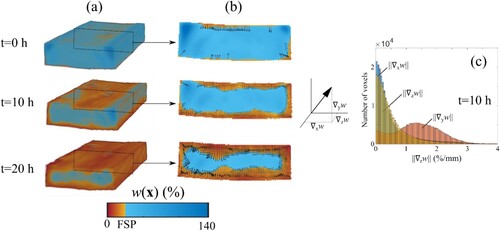
Figure 4 shows an example of the output of the image-processing algorithm. Figure 4(a) shows a three-dimensional representation of the MC distribution within specimen A3 for t = 0 h, t = 10 h, and t = 20 h during the drying schedule S0. For this specimen, the maximal MG as defined in Equation (7) was obtained at t = 20 h. Figure 4(b) shows the two-dimensional MC of the same specimen and times at z = 150 mm, the MG is superimposed as a vector field. In Figure 4(c), a plot represents the histogram of the three orthogonal components of the MG for the 3D MC distribution in (a) at t = 10 h, this Figure also illustrates the inequality in Equation (6).

Figure 4. MC and MG estimation: (a) The 3D MC distribution of specimen A3 at times 0, 10, and 20 h during the drying schedule S0. (b) The 2D MC distribution of the same specimen at the same times at z = 150 mm overlapped with its MG vector field computed with Equation (3) and satisfying the condition $w\left(\mathit{x}\right)<FSP$, represented as dark arrows every 2 voxels in the x and y directions. (c) Histograms of the norm of the three orthogonal components of the MG vector field represented at time 10 h in (b).

3.2. Analysis of moisture gradients

In Figure 5, the average MC and the proportion of high MG values ($P$) with respect to time are plotted, together with the DBT and WBT. It was observed across all specimens and tested schedules that the parameter $P$ increased and peaked before decreasing. The value of the peaks labelled $P_{\mathrm{m}\mathrm{a}\mathrm{x}}$ and the times at which they occurred from the end of the heating regime is given in Figure 6.

Figure 5. Average MC and proportion of high MG values (P) as a function of time (left). Logged parameters of each drying run with the dry-bulb temperature (DBT), wet-bulb temperature (WBT), and relative humidity (RH) (right).

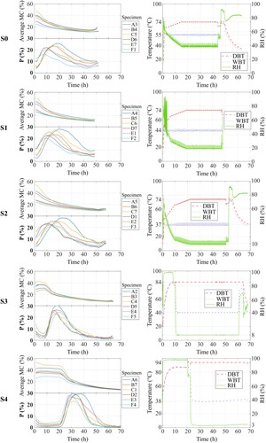
Figure 6. Maximum proportion P_max of MG values $\ge 1\text{\%}/\mathrm{m}\mathrm{m}$ across specimens and schedules. Time of P_max is given from the end of the heating regime.

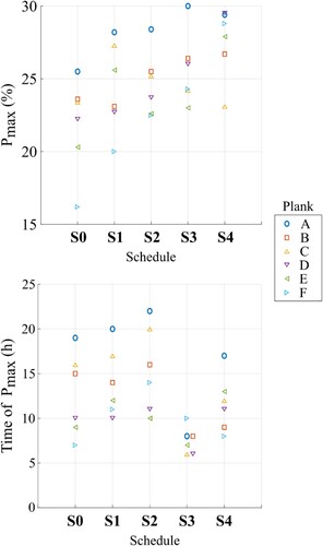
For the schedules S0, S1, and S2, the peaks were achieved during the capillary regime or at the beginning of the diffusion regime. Both the value of $P_{\mathrm{m}\mathrm{a}\mathrm{x}}$ and of the time of the peaks increased when decreasing the RH from schedule S0 to S2. For the specimens with higher average initial MC (from planks A, B, and C) the value $P_{\mathrm{m}\mathrm{a}\mathrm{x}}$ tended to be higher and to occur later than for specimens with lower average initial MC (from planks D, E, and F). For schedules S3 and S4, the peaks were achieved sooner after the end of the heating regime than for schedules S0, S1, and S2. The highest values of $P_{\mathrm{m}\mathrm{a}\mathrm{x}}$ were achieved in the most aggressive schedule (S4).

A comparison of the MG distributions between the specimens dried with schedules S0 and S4 at their respective time of $P_{\mathrm{m}\mathrm{a}\mathrm{x}}$ is given in Figure 7. During the S0 drying run, high MG values were mostly located near the surface of the specimens, which includes the region prone to checking, this was also observed in S1, S2, and S3 and not only at the time at which $P_{\mathrm{m}\mathrm{a}\mathrm{x}}$ occurred, but also afterwards until the end of the schedules. In S4 however, high MG values were not located at the surface but deeper within the specimens. As the drying continued the high MG values receded towards the core of the specimens. To illustrate more this observation, the MC profiles across the thickness of clear wood slices for plank A specimens are plotted in Figure 8.

Figure 7. MG distributions in clear wood cross-sections of the specimens dried with schedules S0 (least aggressive) and S4 (most aggressive). For each specimen, the distribution is plotted at the time of $P_{max}$

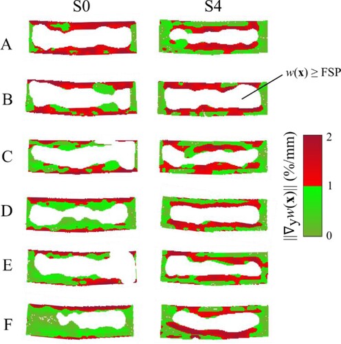
Figure 8. MC profiles across the thickness of clear wood slices of plank A specimens dried with the different schedules. The 2D MC distributions of the chosen slices are shown as coloured maps under the MC profile, the dark line indicates where the MC profile was plotted. The dashed line indicates the MC of FSP.

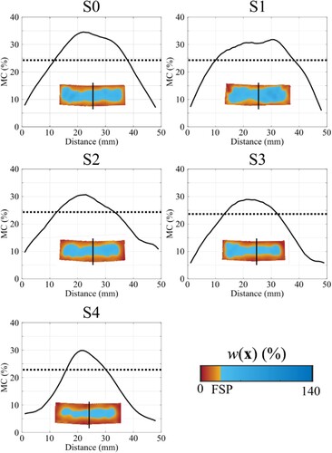
The MC profiles observed in S0, S1, S2, and S3 are typical of Fickian diffusion in which, at the spatial resolution considered, the MC increases somewhat linearly from the surface of the specimens until the depth at which MC values above FSP are estimated. Similar profiles were observed when Scots pine specimens were dried at a DBT of 60°C and RH of 59% (Rosenkilde 2002). The MC profile observed in S4 is characterised by sharp and localised MG that recedes towards the core. Similar MC profiles such as observed in S4 can be found in Chen et al. (1997) where 50 mm thick radiata pine boards were dried at high temperature (DBT of 120°C and WBT of 70°C).

Conclusion

In this study, the potential of 4DCT combined with a newly developed image-processing algorithm was investigated as a tool to evaluate kiln-drying schedules of sawn timber with the aim of optimising industrial drying processes. Centre-yielded plank specimens of Norway spruce were simultaneously CT-scanned and kiln-dried with different schedules with increasingly more aggressive drying conditions and their 4D MC distributions were estimated. This method provides more data than other techniques as the MC can be repetitively estimated in 3D. This allows to estimate the average MC of sawn timber in a non-destructive manner and more accurately than previous CT-based methods that estimated the MC in a single cross-sectional slice of clear wood. Moreover, a new definition of the MG for the sawmill industry is proposed and its reliability is demonstrated.

As the drying rate increased with more aggressive drying conditions, the planks were dried down to the target MC in a faster manner. Indeed, only 10–15 h of drying were necessary to reach the target of 18% MC with the most aggressive schedules (S3 and S4) while 30 h were necessary with the reference schedule (S0). Within the scanned regions and at the spatial resolution of the tomograms, no checking was observed in any of the specimens across the different schedules. This observation suggests that, under the conditions prevailing in this study, centre-yielded planks of Norway spruce can be dried under more aggressive drying conditions than recommended by current drying simulations without causing checking. This does not mean that the drying stresses experienced by the specimens across the different schedules were equivalent, as suggested by the analysis of MG, but that at least they did not exceed a certain threshold leading to cracking. Faster and crack-free drying is desirable and could potentially reduce the energy consumption and improve the efficiency of the process.

Further research is needed to assess if 4DCT can be a general tool to aid in optimising the industrial kiln drying of sawn timber but the first results in this study were promising. It will be possible with this method to investigate moisture transport in all anisotropic directions, this could be particularly interesting in the longitudinal direction and in the vicinity of knots. The method could generate new knowledge about moisture-induced stresses, deformations, and cracking. The possibility of incorporating the 4DCT data into finite element modelling to simulate kiln drying processes should also be considered.

Disclosure statement

No potential conflict of interest was reported by the author(s).

References

- Aichholzer, A., et al., 2018. Microwave testing of moist and oven-dry wood to evaluate grain angle, density, moisture content and the dielectric constant of spruce from 8 GHz to 12 GHz. European Journal of Wood and Wood Products, 76, 89–103.
- Andersson, J.-E., et al., 2011. “State of the art–Energianvändning i den svenska sågverksindustrin.”.
- Avramidis, S., Lazarescu, C., and Rahimi, S., 2023. Basics of wood drying. Chapter 13. In: P. Niemz, A. Teischinger and D. Sandberg (Eds.), Springer Handbook of Wood Science and Technology. Springer, 679–706.
- Awais, M., et al., 2022. Quantitative prediction of moisture content distribution in acetylated wood using near-infrared hyperspectral imaging. Journal of Materials Science, 57 (5), 3416–3429.
- Beaulieu, J., and Dutilleul, P., 2019. Applications of computed tomography (CT) scanning technology in forest research: a timely update and review. Canadian Journal of Forest Research, 49 (10), 1173–1188.
- Benson-Cooper, D., and Knowles, R., 1982. Computed Tomographic Scanning for the Detection of Defects within Logs. FRI Bulletin No. 8. Forest Research Institute, Rotorua, New Zealand.
- Chen, G., Keey, R., and Walker, J., 1997. The drying stress and check development on high-temperature kiln seasoning of sapwood Pinus radiata boards: Part I: moisture movement and strain model. Holz als Roh-und Werkstoff, 55 (2-4), 59–64.
- Couceiro, J., 2019. X-ray computed tomography to study moisture distribution in wood. PhD Thesis, Luleå University of Technology, Skelelfteå, Sweden.
- Esping, B., 1988. Trätorkning. 2, Torkningsfel-åtgärder. Trätek.
- Florisson, S., et al., 2022. Macroscopic X-ray computed tomography aided numerical modelling of moisture flow in sawn timber. European Journal of Wood and Wood Products, 80 (6), 1351–1365.
- Florisson, S., Ormarsson, S., and Vessby, J., 2019. A numerical study of the effect of green-state moisture content on stress development in timber boards during drying. Wood and Fiber Science, 51 (1), 41–57.
- Freyburger, C., et al., 2009. Measuring wood density by means of X-ray computer tomography. Annals of Forest Science, 66 (8), 804.
- Hansson, L., and Fjellner, B.-A., 2013. Wood shrinkage coefficient and dry weight moisture content estimation from CT-images. Pro Ligno, 9 (4), 557–561.
- Hewitt, E., and Hewitt, R.E., 1979. The Gibbs-Wilbraham phenomenon: an episode in Fourier analysis. Archive for History of Exact Sciences, 21 (2), 129–160.
- Johnson, A., 2010. Polygon Clipping and Offsetting Library. Available from: http://www.angusj.com/clipper2/Docs/Overview.htm.
- Klein, S., et al., 2010. Elastix: a toolbox for intensity-based medical image registration. IEEE Transactions on Medical Imaging, 29 (1), 196–205.
- Konopka, A., et al., 2021. Mathematical model of the energy consumption calculation during the pine sawn wood (Pinus sylvestris L.) drying process. Wood Science and Technology, 55 (3), 741–755.
- Lanvermann, C., et al., 2014. Combination of neutron imaging (NI) and digital image correlation (DIC) to determine intra-ring moisture variation in Norway spruce. Holzforschung, 68 (1), 113–122.
- Lindgren, O., 1985. Preliminary observations on the relationship between density/moisture content in wood and X-ray attenuation in computerised axial tomography. In: Proceedings of the 5th Nondestructive Testing of Wood Symposium, Pullman, Washington, USA. Date and Editors.
- Miettinen, A., et al., 2016. Time-resolved X-ray microtomographic measurement of water transport in wood-fibre reinforced composite material. In: IOP Conference Series: Materials Science and Engineering, IOP Publishing.
- Mull, R.T., 1984. Mass estimates by computed tomography: physical density from CT numbers. American Journal of Roentgenology, 143 (5), 1101–1104.
- Niemz, P., Teischinger, A., and Sandberg, D., 2023. Springer handbook of wood science and technology. Springer.
- Oliveira, F.P., and Tavares, J.M.R., 2014. Medical image registration: a review. Computer Methods in Biomechanics and Biomedical Engineering, 17 (2), 73–93.
- Patera, A., et al., 2018. A non-rigid registration method for the analysis of local deformations in the wood cell wall. Advanced Structural and Chemical Imaging, 4 (1), 1–11.
- Poupet, B., et al., 2022. Moisture gradient analysis during sawn timber drying. In: The 18th Annual Meeting of the Northern European Network for Wood Science and Engineering, Brischke, C. & Buschalsky, A. (Eds.), 21–22 September 2022, Göttingen, Germany, 171–173.
- Poupet, B., et al., 2023. Estimation of moisture distribution in sawn timber using computed tomography. In: World Conference on Timber Engineering.
- Riley, S., Harrington, J., and Elustondo, D., 2022. A theoretical analysis of the potential effect of negative pressure in wood drying based on a CT-scanner study. Drying Technology, 40 (14), 2975–2989.
- Rosenkilde, A., 2002. Moisture content profiles and surface phenomena during drying of wood (Doctoral dissertation, Byggvetenskap).
- Salin, J., 1999. Simulation models; from a scientific challenge to a kiln operator tool. In: 6 th International IUFRO Wood Drying Conference.
- Salmen, L., 1982. Temperature and water induced softening behaviour of wood fiber based materials, Department of Paper Technology, Royal Institute of Technology Stockholm.
- Sanabria, S.J., et al., 2015. Adaptive neutron radiography correlation for simultaneous imaging of moisture transport and deformation in hygroscopic materials. Experimental Mechanics, 55, 403–415.
- Standards Sweden. 2004. Moisture content of a piece of sawn timber - Part 1: Determination by oven dry method (SS-EN 13183-1/AC:2004).
- Stevens, W.C., and Pratt, G.H., 1961. Kiln operators handbook. A guide to the kiln drying of timber. Department of Scientific & Industrial Research, Forest Products Research, London, UK.
- Wang, Q., et al., 2019. Non-destructive detection of density and moisture content of heartwood and sapwood based on X-ray computed tomography (X-CT) technology. European Journal of Wood and Wood Products, 77 (6), 1053–1062.
- Watanabe, K., et al., 2008. Non-destructive measurement of moisture distribution in wood during drying using digital X-ray microscopy. Drying Technology, 26 (5), 590–595.
- Wiberg, P., and Morén, T.J., 1999. Moisture flux determination in wood during drying above fibre saturation point using CT-scanning and digital image processing. Holz als Roh-und Werkstoff, 57, 137–144.
- Withers, P.J., et al., 2021. X-ray computed tomography. Nature Reviews Methods Primers, 1 (1), 18.
- Xu, K., et al., 2017. Determination of moisture content and moisture content profiles in wood during drying by low-field nuclear magnetic resonance. Drying Technology, 35 (15), 1909–1918.