Economic lifetime prediction of a mining drilling machine using an artificial neural network

Abstract

This study develops models for predicting the economic lifetime of drilling machines used in mining. It uses three cases, each represented by a MATLAB code, to develop an optimisation model. The resulting ORT is fed as input to an artificial neural network (ANN) and the results translated into a relatively simple equation. The study finds that increasing the purchase price and decreasing the operating and maintenance costs will increase a machine’s ORT linearly. Decreased maintenance cost has the largest impact on ORT, followed by increased purchase price and decreased operating cost. The ANN method gives a series of basic weight and response functions which can be made available to any engineer without the use of complicated software. It also helps decision-makers determine the best time economically to replace an old machine with a new one; thus, it can be extended to more general applications in the mining industry.

Keywords:

• artificial neural network
• decision support system
• mining drilling machine
• optimisation model
• replacement time

1. Introduction

Mining is a large, integrated, automated and complex industry; having safe, reliable and cost-effective production is a strategic necessity if a company is to meet customer requirements and gain a competitive advantage globally. Mining industries are under constant pressure to improve their production performance at minimum cost. On the one hand, they need more reliable capital equipment with higher performance capabilities; on the other hand, these are more expensive.

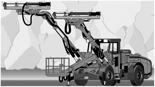
Drilling machines are a key element of mining production, especially in the mineral extracting process (see Figure 1). These machines are subject to degradation throughout their operating life; this reduces production rates, with a resulting negative economic effect. In addition, because drilling machines are used in underground mines, they are subjected to a harsh working environment, thereby accelerating degradation. A key question for mining companies is when to replace the drilling machines to minimise cost and maximise profit.

Figure 1. Drilling machine.

As operating and maintenance costs are the main contributing factors to the total cost, researchers concerned with cost optimisation are especially interested in the optimum replacement time of production and repairable equipment, defined as the time at which the total cost is minimised [1]. For example, Ahmadi and Kumar [2] developed a cost rate function to identify the optimum interval and frequency of inspection and restoration of an aircraft’s repairable but ageing components whose failures are hidden. Wijaya et al. [3] proposed a robust-optimum multi-attribute age-based replacement policy. A model for estimating the lifetime of mill liners was developed by Dandotiya and Lundberg [4] based on the properties of the ore used. Their proposed lifetime model is combined with a replacement interval model to determine the optimum replacement interval for the mill liners; it considers process parameters of multiple ore types.

Some researchers have considered the optimal lifetime of capital equipment using economic theories and vintage capital models, represented mathematically by non-linear Volterra integral equations with unknown limits of integration [5–8]. Others have used the theory of dynamic programming to consider technological changes under finite and infinite time horizons [9–12]. For instance, Yatsenko and Hritonenko [13] studied the lifetime optimisation of capital equipment using integral models; they designed a general investigation framework for optimal control of the models. Hartman and Murphy [14] suggested a dynamic programming approach to the finite time-horizon equipment replacement problem with stationary cost. Their model considers the relationship between the infinite time-horizon solution (continuous replacement of equipment at the end of its economic lifetime) and the finite time-horizon solution. Hritonenko and Yatsenko [15] constructed a computational algorithm to solve a nonlinear integral equation; the solution helps determine the optimal policy of equipment replacement given the technological advances. Finally, Kärri [16] considered the optimal replacement time of an old machine by modelling the costs of the old machine with simple linear functions. The resulting optimisation model minimises the machine cost and maximises the profit. It can handle capacity expansion and replacement situations.

The artificial neural network (ANN) has been widely touted as solving many forecasting and maintenance decision modelling problems. For example, Gebraeel et al. [17] proposed a set of neural network models using exponential approximations to estimate the remaining life of thrust ball bearings in real time. Later, Wu et al. [18] developed an integrated neural network-based decision support system for predictive maintenance of rotational equipment. The integrated system is platform-independent and is aimed at minimising the expected cost per unit operational time. Jafar et al. [19] used an application of ANN to model the failure rate and estimate the optimal replacement time for individual pipes in an urban water distribution system.

Other researchers have studied the remaining life predictions of various components using ANN [20–22]. For example, Ahmadzadeh and Lundberg [23] developed a method which predicts the remaining useful life of grinding mill liners. Using this method, there is no need to stop the mill, enter it and measure the liners’ wear to make appropriate maintenance decisions, leading to enormous monetary savings.

Although many studies have estimated the optimal lifetime of equipment considering the possibility of technological change, more practical methods of ORT prediction are required. It is well known that ANNs are able to model easily any type of parametric or non-parametric process and automatically transform the input data into optimal and accurate outputs, in this case, the ORT of a drilling machine. In addition, using a neural network gives a clear picture of the relative importance of the input variables and suggests how variations in inputs will affect the ORT. Finally, because the neural network can be represented by a series of basic weight and response functions, the results can be made available to any engineer without the need for complicated software.

The present study develops an ANN-based optimisation model using available cost data to estimate the ORT of a drilling machine. The available cost data are the machine purchase price, maintenance costs and operating costs. The production loss cost of machine downtime is not considered due to the availability of a spare drilling machine in the case study. The overall goal of model development is to minimise costs in the mining industry.

2. Data collection

Four years of cost data were collected in a Maximo computerised maintenance management system. Since drilling is not a continuous process, the operating cost can be estimated by considering the utilisation of the machine. Data include corrective maintenance costs (CM), preventive maintenance costs (PM) and repair time. The corrective and preventive maintenance costs comprise spare parts costs (SP) and labour costs (LC), calculated as real costs without inflation.

3. Optimal replacement time prediction using ANN

ANNs can perform nonlinear modelling without prior information and are able to learn complex relationships between inputs and outputs; the process is also fast. One of the first successful applications of ANNs in forecasting was reported by Zhang et al. [24]; these researchers designed a feedforward ANN to accurately simulate a chaotic series. In general, feedforward ANNs trained with the back propagation algorithm have been found to perform better than classical autoregressive models for trend prediction in a nonlinear time series [25,26].

In this study, ANN is applied to find nonlinear or linear relationships between inputs (costs) and outputs (ORT) for a drilling machine. The proposed ANN model combines multi-layer perceptions with the back-propagation Levenberg-Marquardt algorithm. In function approximation problems, this algorithm is considered to have the fastest convergence and is one of the most powerful learning algorithms [25,27].

The analyses are based on three cases, increasing purchase price (IPP), decreasing operating cost (DOC) and decreasing maintenance cost (DMC), each represented by a MATLAB code. The resulting ORT is fed as input to ANN and the results translated into a relatively simple equation. The equation is transformed to an Excel spreadsheet to make ORT estimation quick and easy for any engineer to apply.

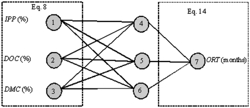
As noted above, the proposed model has three inputs: the increased purchase price (IPP (%)), decreased operating cost (DOC (%)) and decreased maintenance cost (DMC (%)). A hidden layer with three neurons and a nonlinear transfer function allows the network to learn nonlinear and linear relationships between input and output variables. The number of neurons in the output layer is constrained to one, as the output only requires one parameter, in this case, the ORT of the drilling machine.

The number and size of layers between network inputs and the output layer are determined by testing several combinations of numbers of layers and various numbers of neurons in each layer. Each of the selected combinations is tested with several different initial conditions to guarantee the proposed model is the best solution. The structure of the optimal ANN model is shown in Figure 2.

Figure 2. Optimal structure of ANN model.

4. Calculation of the ANN inputs

The optimal value for costs is required to obtain the ORT using ANN, so the following optimisation model is developed to find the replacement time (RT) that minimises the total cost value (), as shown in Equation (6(6) ). The term ‘total cost value’ is defined as the summation of the machine purchase price (PP), operating cost (OC), maintenance cost (MC) and resale value S (t) over a long period, with replacements occurring at intervals of n periods. Therefore,(1)

(2) (3)

(4)

where a represents the percentage that is multiplied by the machine purchase price to represent the machine’s value on the first day of use. During discussions, a group of experts agreed the machine’s purchase price decreases by 10% at this time. The depreciation rate that allows for full depreciation by the end of the planned lifetime of the machine is modelled by Equation (5(5) ) [28]:(5) (6)

where(7)

MATLABTM^TM software is used to enable a variation of the parameter RT of Equation (6(6) ) for the optimisation time horizon in order to identify the ORT of a drilling machine that minimises. The results show that the lowest possible can be achieved by replacing the machine every 96 months.

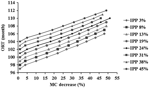
When MATLAB codes are used to identify the effect of IPP, DOC and DMC on the optimal age of replacement, in all cases, the purchase price increases while the operating and maintenance costs decrease (e.g. Figure 3). Case one represents the effect of IPP from (1–50)% with DOC and DMC at different percentages. Case two represents the effect of DOC from (1–50)% with DMC and IPP at different percentages. Case three represents the effect of DMC from (1–50)%, with IPP and DOC at different percentages. For greater clarity, part of case three is selected (Figure 3) to show the simultaneous production of (1–50)% DMC and 7% DOC and IPP at different percentages. For this case alone, 400 different input data for ANN are considered. The procedure is repeated for all cases, producing 6150 data-sets.

Figure 3. Producing 400 input data for ANN as part of case three.

The produced data-sets (6150 data) from these codes are treated as inputs for the proposed ANN model to predict the ORT of the drilling machine at any percentage of IPP or DMC and DOC.

5. Training and testing the proposed ANN model

Pre-processing data by scaling improves the training of the neural network. To avoid a slow rate of learning, specifically near the end points of the output range (due to the property of the sigmoid function, which is asymptotic to values 0 and 1), the input and output data are scaled between the interval 0.1 and 0.9 [29]. It should be noted that any new input data should be scaled before being presented to the network and the corresponding predicted values should be un-scaled before use [30]. The linear scaling equation is expressed by:(8)

where X_s represents the scaled value of input variables and X represents the un-scaled value of input variables. The input variables are IPP, DOC and DMC. Equation (8(8) ) is used here for an IPP, DOC and DMC between minimum increasing or decreasing percentage 1% (X_min) and maximum increasing or decreasing percentage 50% (X_max), such that

(9)

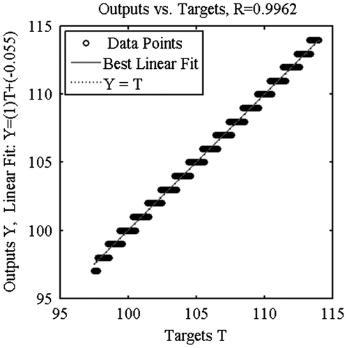
From the 6150 scaled data, 90% are used in the training of the neural network; see Figure 4. The model shown in Figure 4 has very high values of R² = 0.9962 for ANN. However, as also shown in the figure, the neural network model yields outputs very close to the desired targets with high accuracy.

Figure 4. Learning capability: Output of the proposed ANN for seen data.

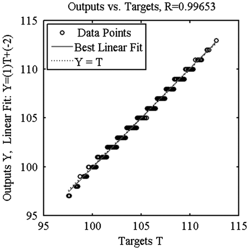
After the training is completed, the network is tested for its learning and generalisation capabilities. Its learning ability is tested by examining its ability to produce outputs for the set of inputs (seen data) used in the training phase. Its generalisation ability is tested by investigating its ability to respond to the input sets (unseen data) not included in the training process; thus, 10% are used for tests with the obtained network (Figure 5). As evident in Figure 5, the model has very high values of R² = 0.99653 for ANN. However, the neural network model also yields outputs very close to the desired targets with high levels of certainty.

Figure 5. Generalisation capability: Output of the proposed ANN for unseen data.

6. Results and discussion

The proposed ANN model is used to design a formula to calculate the ORT of a drilling machine. The structure of the optimal ANN model is shown in Figure 2; its connection weights and threshold levels are summarised in Table 1.

Table 1. Weights and threshold levels for the proposed ANN.

Hidden layer nodes	wii weights from node ith input layer to node jth hidden layer			Hidden threshold (θj)
	i = 1	i = 2	i = 3
j=4	−0.0648	−0.03030	−0.1297	10.4780
j=5	−2.6814	−0.78166	−2.1337	0.18142
j=6	−1.2496	−0.8258	−2.3112	5.023854
Output layer nodes	wij weights from node ith hidden layer to node jth output layer			Output threshold (θj)
	i = 4	i = 5	i = 6
j=7	7.795	−5.3591	−10.801	2.919081

The equation length depends on the number of nodes in the hidden layer. Adopting three nodes gives an accuracy of 99%. The small number of connection weights of the neural network enables the ANN model to be translated into a relatively simple formula, in which the predicted ORT can be expressed as follows:

(10)

where ORT_s represents the scaled ORT derived from the ANN model, θ_j represents the output threshold and w_ij represents the weight from node i in the hidden layer to node j in the output layer. Hence,

(11) (12) (13)

Note that before using Equations (10(10) –13(13) ), all input variables need to be scaled between 0.1 and 0.9 using Equation (8(8) ). It should also be noted that the predicted ORT_s obtained from Equation (10(10) ) is scaled between 0.1 and 0.9; however, in order to obtain the actual value of ORT, it must be re-unscaled using the following formula:(14)

Equation (14(14) ) is obtained by solving Equation (8(8) ), considering the input variable (X) as unknown and the output variable (X_s) as known. An Excel spreadsheet can be used as a substitute for fast and accurate calculation of the ORT. Equation 15(15) is applied to estimate the actual value of the ORT of the drilling machine as follows:(15)

where ORT_max and ORT_min represent the maximum and minimum values of ORT derived from the optimisation model.

6.1. Study of relative importance of input parameters

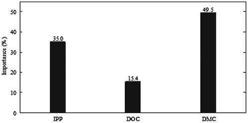
The method of partitioning weights, proposed by Garson [31] and adopted by Goh [32], is now used to determine the relative importance of the various input parameters; see Figure 6.

Figure 6. Relative importance of the variables affecting the ORT of the drilling machine.

As evident in Figure 6, the most important parameter influencing the ORT of the drilling machine is the DMC, followed by the IPP. The DOC has the least influence. The design for reliability and maintainability should be adapted to reduce the maintenance cost, thus increasing the ORT of the drilling machine.

6.2. Study of variables influencing the ORT of the drilling machine

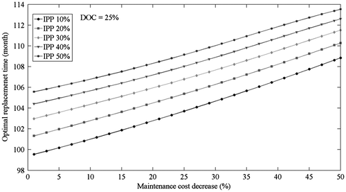
With applying Equation 15(15) , the ORT of drilling machine is calculated for different variables, including IPP, DOC and DMC, to see the influence of these variables. The DMC is the most important factor, as shown in Figure 6. Generally, the ORT increases with a decrease in maintenance cost, compatible with the results shown in Figures 7 and 8.

Figure 7. Effect of IPP and DMC for 25% OC decrease.

Figure 8. Effect of DOC and DMC for 25% PP increase.

6.3. Effect of increasing machine purchase price

As Figure 6 shows, the second most influential variable on the ORT is the machine’s IPP. The correlation of IPP and DMC when the cost of operating is reduced by 25% is shown in Figure 7. As is evident, both IPP and DMC have a positive effect on increasing the ORT.

6.4. Effect of decreasing machine operating cost

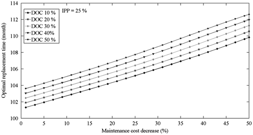
Figure 8 shows the correlation of DOC and DMC for a given 25% increase in PP. Clearly, both DOC and DMC have a positive effect on increasing the ORT.

7. Conclusions

The main advantage of the proposed neural network model is its ability to produce acceptable results: the correlation between input and output variables is very high and the accuracy is more than 99%. Moreover, the model’s performance is very consistent for data used for training (seen) and testing (unseen). Therefore, it is very effective in estimating and predicting the ORT of a mining drilling machine. Further, because the ANN model uses a series of basic weight and response functions, it does not require expensive and sophisticated equipment for data recording and analysis.

The predicted ORT from the ANN model indicates that increasing the purchase price and decreasing the operating and maintenance costs will increase the ORT of the drilling machine. Results also show that the maintenance cost has the largest impact on the ORT, followed by the purchase price and operating cost. Hence, the manufacturer must make a greater effort to improve the reliability and maintainability of the drilling machine to reduce the costs associated with maintenance and increase the ORT.

This study presents a comprehensive and very practical approach using ANN which can provide the economic replacement time of a drilling machine with higher levels of certainty. It helps engineers and decision-makers determine when it is best to economically replace an old machine with a new one without using complicated software. Because of its effectiveness and simplicity, the model can be extended to more general applications in the mining industry. The dynamic nature of the proposed methodology opens up future studies of economic lifetime prediction for different categories of mining equipment.

Notations
ORT	=	optimal replacement time (months)
ANN	=	artificial neural network
CM	=	corrective maintenance cost (CU)
CU	=	currency unit
PM	=	preventive maintenance cost (CU)
IPP	=	increase purchase price (%)
DOC	=	decrease operating cost (%)
DMC	=	decrease maintenance cost (%)
RT	=	replacement time (months)
TCvalue	=	total cost value (CU)
PP	=	purchase price (CU)
OC	=	operating cost (CU)
MC	=	maintenance cost (CU)
S(t)	=	resale value (CU)
SPc	=	spare part cost for corrective maintenance (CU)
LCc	=	labour cost for corrective maintenance (CU)
SPp	=	spare part cost for preventive maintenance (CU)
LCp	=	labour cost for preventive maintenance (CU)
Dr	=	depreciation rate
t	=	machine lifetime (months)
SV	=	scrap value (CU)
BV1	=	booking value on first day of operation (CU)
L	=	planned lifetime (month)
N	=	number of machine replacements
T	=	optimisation time horizon (120 months)
Xs	=	scaled value of input variables
∆	=	difference between maximum and minimum values of input variables
X	=	unscaled value of input variables
Xmax	=	maximum value of input variables
Xmin	=	minimum value of input variables
θj	=	output threshold
wij	=	weight from node i in the hidden layer to node j in the output layer

Acknowledgement

The authors would like to thank Boliden AB, Atlas Copco for supporting this research. Special appreciation is extended to the operating and maintenance engineers at Boliden AB for sharing their valuable knowledge, experience and data to improve this study. The authors would also like to thank Majid Al-Gburi, Alireza Ahmadi for their help.

References

- A.K.S. Jardine and A.H.C. Tsang, Maintenance, Replacement, and Reliability Theory and Applications, Taylor & Francis Group, New York, 2006.
- A. Ahmadi and U. Kumar, Cost based risk analysis to identify inspection and restoration intervals of hidden failures subject to aging, IEEE Trans. Reliab. 60 (2011), pp. 197–209.10.1109/TR.2011.2104530
- A.R. Wijaya, J. Lundberg, and U. Kumar, Robust-optimum multi-attribute age-based replacement policy, J. Qual. Maint. Eng. 18 (2012), pp. 325–343.10.1108/13552511211265910
- R. Dandotiya and J. Lundberg, Economic model for maintenance decision: a case study for mill liners, J. Qual. Maint. Eng. 18 (2012), pp. 79–97.10.1108/13552511211226201
- R. Boucekkine, M. Germain, and O. Licandro, Replacement echoes in the vintage capital growth model, J. Econ. Theory. 74 (1997), pp. 333–348.10.1006/jeth.1996.2265
- T.F. Cooley, J. Greenwood, and M. Yorukoglu, The replacement problem, J. Monetary Econ. 40 (1997), pp. 457–499.10.1016/S0304-3932(97)00055-X
- N. Hritonenko and Y. Yatsenko, Applied Mathematical Modeling of Engineering Problems, Massachusetts: Kluwer Academic Publishers, 2003.10.1007/978-1-4419-9160-7
- N. Hritonenko, Optimization analysis of a nonlinear integral model with applications to economics, Nonlinear Stud. 12 (2005), pp. 59–72.
- R. Bellman, Equipment replacement policy, J. Soc. Ind. Appl. Math. 3 (1955), pp. 133–136.
- E.J. Elton and M.J. Gruber, On the optimality of an equal life policy for equipment subject to technological improvement, J. Oper. Res. Q. 27 (1976), pp. 93–99.10.1057/jors.1976.9
- G. Bethuyne, Optimal replacement under variable intensity of utilization and technological progress, Eng. Econ. 43 (1998), pp. 85–105.10.1080/00137919808903191
- N. Hritonenko and Y. Yatsenko, The dynamics of asset lifetime under technological change, Oper. Res. Lett. 36 (2008), pp. 565–568.10.1016/j.orl.2008.04.003
- Y. Yatsenko and N. Hritonenko, Optimization of the lifetime of capital equipment using integral models, J. ind. manage. optim. 1 (2005), pp. 415–432.10.3934/jimo
- J.C. Hartman and A. Murphy, Finite-horizon equipment replacement analysis, IIE Trans. 38 (2006), pp. 409–419.10.1080/07408170500380054
- N. Hritonenko and Y. Yatsenko, Integral equation of optimal replacement: Analysis and algorithms, Appl. Math. Model. 33 (2009), pp. 2737–2747.10.1016/j.apm.2008.08.007
- T. Kärri, Timing of Capacity Change: Models for Capital Intensive Industry, Lappeenranta: Lappeenrannan teknillinen yliopisto/Lappeenranta University of Technology, 2007.
- N. Gebraeel, M. Lawley, and R. Liu, Vibration-based condition monitoring of thrust bearings for maintenance management, Intell. Eng. Syst. Artif. Neural Networks 12 (2002), pp. 543–551.
- S. Wu, N. Gebraeel, M.A. Lawley, and Y. Yih, A neural network integrated decision support system for condition-based optimal predictive maintenance policy, IEEE Trans. Syst. Man Cybern. Part A Syst. Humans 37 (2007), pp. 226–236.10.1109/TSMCA.2006.886368
- R. Jafar, I. Shahrour, and I. Juran, Application of Artificial Neural Networks (ANN) to model the failure of urban water mains, Math. Comput. Model. 51 (2010), pp. 1170–1180.10.1016/j.mcm.2009.12.033
- C.S. Byington, M. Watson, and D. Edwards, Data-driven neural network methodology to remaining life predictions for aircraft actuator components, IEEE Aerosp. Conf. Proc. 6 (2004), pp. 3581–3589.
- M. Mazhar, S. Kara, and H. Kaebernick, Remaining life estimation of used components in consumer products: Life cycle data analysis by Weibull and artificial neural networks, J. Oper. Manage. 25 (2007), pp. 1184–1193.10.1016/j.jom.2007.01.021
- F. Ahmadzadeh and J. Lundberg, Application of multi regressive linear model and neural network for wear prediction of grinding mill liners, Int. J. Adv. Comput. Sci. Appl. 4 (2013), pp. 53–58.
- F. Ahmadzadeh and J. Lundberg, Remaining useful life prediction of grinding mill liners using an artificial neural network, Minerals Eng. 53 (2013), pp. 1–8.10.1016/j.mineng.2013.05.026
- G. Zhang, B. Eddy Patuwo and M.Y. Hu, Forecasting with artificial neural networks, Int. J. Forecast. 14 (1998), pp. 35–62.10.1016/S0169-2070(97)00044-7
- S. Hykin, Neural Networks: A Comprehensive Foundation, 2nd ed., New Jersey: Printice-Hall, 1999.
- R. Yam, P. Tse, L. Li, and P. Tu, Intelligent predictive decision support system for condition-based maintenance, Int. J. Adv. Manuf. Technol. 17 (2001), pp. 383–391.10.1007/s001700170173
- G.P. Zhang and M. Qi, Neural network forecasting for seasonal and trend time series, Eur. J. Oper. Res. 160 (2005), pp. 501–514.10.1016/j.ejor.2003.08.037
- B. Luderer, V. Nollau, and K. Vetters, Mathematical formulas for economists, Berlin: Springer Heidelberg, 2010.10.1007/978-3-642-04079-5
- A.W.C. Oreta, Simulating size effect on shear strength of RC beams without stirrups using neural networks, Eng. Struct. 26 (2004), pp. 681–691.10.1016/j.engstruct.2004.01.009
- S.T. Yousif, Artificial neural network modeling of elasto-plastic plates, Ph.D. thesis, College of Engineering, Mosul University, 2007.
- G.D. Garson, Interpreting neural-network connection weights, Artif. Intell. 6 (1991), pp. 46–51.
- A. Goh, Back-propagation neural networks for modeling complex systems, Artif. Intell. Eng. 9 (1995), pp. 143–151.10.1016/0954-1810(94)00011-S