Exploring the capabilities of portable device photogrammetry for 3D surface roughness evaluation

ABSTRACT

The feasibility of using a portable photogrammetric device to digitalise rock surface roughness is investigated. Structured light 3D scanner, terrestrial LiDAR scanner, and portable photogrammetry device are used to scan precast different roughness lab-scale specimens. The reconstructed 3D surface is evaluated for accuracy using point cloud distance, joint roughness coefficient, and 3D roughness parameters. Results show that the portable device can reconstruct a 3D model comparable in accuracy to a structured light 3D scanner in 15 minutes. The proposed method is applied to laboratory-scale model reconstruction, with the potential to scan rock surfaces efficiently and economically in a mine.

KEYWORDS:

• Surface roughness
• photogrammetry
• point cloud

1. Introduction

Rock surface characteristics significantly affect rockmass behaviour and properties, such as their strength, stability, and deformability, as well as joint frictional properties, shear and bond strengths. Accurate measurement of surface roughness on rocks is important for assessing geotechnical stability, rock quality, and the effectiveness of surface treatment. It also provides valuable insights into rock formation processes and assists in modelling and predicting the interaction between rocks and other materials, such as water. Several techniques to measure and quantify the rock surface roughness have been developed, such as profilometers [1], 3D laser scanners [2–5], and photogrammetry [6,7].

The rock joint roughness coefficient (JRC) [8] is widely used to quantify rock joint roughness when assessing the shear strength of rock discontinuities. JRC is two-dimensional and subjective to user interpretation [9]. The JRC values are typically estimated by visual comparison against ten Barton’s standard profiles [8]. The visual comparison against Barton’s standard profiles has been enhanced by measuring the roughness from digitised profiles [1,10,11]. Several scholars have developed algorithms to automate the JRC calculation supported by parameters obtained from digitised profiles. Parameters such as Z₂ [12], R_p [13], and ${\theta }_{max}^{\hspace{0.17em}}/\left(C+1\right)$ [14] have achieved the best results for JRC calculation. JRC has also been applied for quantifying the roughness of 3D surfaces [14–16]. One way of achieving this is by obtaining several equally-spaced line profiles along a specific direction of the surface, determining the JRC of each line profile and averaging the values to represent the JRC of the surface. Such a JRC value only represents the roughness of the specific surface direction. Another way of determining the JRC of 3D surfaces is by extracting line profiles at certain degree intervals using the centre of the surface as the circle centre and then calculating the average value as the JRC of the whole surface [14,17]. These methods are still constrained by the 2D surface line profile and Barton’s standard profiles.

Grasselli [18] proposed a new 3D roughness parameter ${\theta }_{max}^{\hspace{0.17em}}/C$, to assess the roughness of a surface, and then improved to ${\theta }_{max}^{\hspace{0.17em}}/\left(C+1|\right)$ by Tatone [19]. They considered the contact area and dip angle of the shear interface and assumed that only the contact area facing the shear direction provides the shear strength. The value of ${\theta }_{max}^{\hspace{0.17em}}/\left(C+1\right)$ ranges from 0 for a completely smooth surface to ${\theta }_{max}^{\hspace{0.17em}}$ for a saw tooth surface with an inclination between 0${ }^{\circ }$ to 90${ }^{\circ }$.

Different imaging technologies, such as 3D laser or structured light 3D scanners [3,20,21], have been recently used for digitising 2D surface line profiles or 3D surfaces. However, the expensive cost, limited portability, and complicated setup process of 3D scanners contributed to increased costs and complexities in operation. Although LiDAR scanners [5,22,23] have been applied in many field-scale industrial engineering applications, they do not typically offer a millimetre-level accuracy for a relatively large area. While digitalising rock surfaces has been relatively extensively studied, limited attention has been paid to evaluating the smartphone photogrammetric technique capacity, a cost-effective method to digitalise surfaces, for computing surface roughness.

The photogrammetry technique is used to collect high-resolution datasets. These datasets generate a point cloud of rock surface to produce a 3D model, which can be coupled with textural information. The structure from motion (SfM) algorithm [24] is widely used for producing 3D models from high-resolution photogrammetric datasets. SfM is more efficient and flexible than traditional matching algorithms [7]. It rebuilds 3D models with a fixed workflow: aligning images, building dense point clouds, meshing, and texturing, which has been proven to rebuild accurate models on laboratory and field scales [4,24–26].

With the advancement of photography technology, portable photographic equipment, such as smartphones, are now equipped with high-resolution lenses and powerful processors that can provide high-quality images for photogrammetric measurements. Researchers used smartphones to acquire high-resolution geomorphological data in fieldwork [27–29]. Jaud et al. [30] demonstrated that smartphone photogrammetry has the potential for coastal monitoring. An et al. [31] and Fang et al. [32] applied smartphone photogrammetry for the measurement of rock surface and particle size. Furthermore, they developed a multismartphone measurement system for slope and landslide model tests [33,34]. An et al. [7] tested several smartphones to obtain images of rock specimens. They compared the photogrammetric models with those obtained by a laser scanner and concluded that the accuracy of the smartphone photogrammetric method was comparable to that of the laser scanner on a laboratory scale [19]. Such high-quality images are used to directly generate point clouds or 3D mesh files using different specialised applications, such as Polycam (Polycam Inc.), which generates a 3D model by a circle of photos taken from the object [4,35]. Compared with traditional computer software, such as PhotoModeler Premium [36], Metashape [31], and Meshroom [37], Polycam relies on cloud computing to dramatically reduce the time required to create 3D models, often generating them in less than 20 minutes.

3D point cloud comparison has been used to measure surface changes and track the evolution of natural surfaces in surveying techniques. The multiscale model-to-model cloud comparison (M3C2) algorithm [38] is broadly used to assess the difference between two point clouds and evaluate complex topography. It is particularly valuable in applications such as 3D surface reconstruction and shape analysis. It assesses surface changes by measuring the orthogonal distance between point clouds [4,7,38]. It avoids meshing or gridding the point clouds and adapts to missing data or variation in point density. M3C2 has been applied to compute topography changes for natural scenes, such as bedrock gorges, moraines, and rock glaciers [24,39–41].

Smartphones, as common portable devices, have been explored for their application in digitising rock surfaces and quantifying roughness. Previous methods involved capturing images with a smartphone and transferring them to a computer for 3D model construction, while consuming a significant amount of time during the transmission and modelling processes. This study directly utilised a smartphone application for photogrammetry and 3D model reconstruction of grout specimens with different roughness. Then, the reconstructed 3D surface was compared to those obtained by the structured light 3D scanner and terrestrial laser scanner (TLS), and the accuracy of photogrammetry was assessed in two aspects: the point cloud distance and quantitative parameters of surface roughness. It was found that smartphone photogrammetry not only significantly reduced the time required for image transfer and modelling but also achieved surface accuracy comparable to that of a structured light 3D scanner. The limitations of the methods are also discussed.

2. Materials and methods

2.1. Specimens

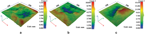
Three 100 mm × 100 mm surfaces with different roughnesses were used in this research, defined as smooth, intermediate, and rough surfaces based on their waviness, unevenness, and elevation. These surfaces were prepared based on natural rock joint surfaces scanned by a structured light 3D scanner, EinScan Pro 2X. Since a light source scanner was used for imaging, the scanning process was conducted indoors to avoid the impact of other light sources. Sets of the point cloud from the scanning data of original rock surfaces were generated, as shown in Figure 1. The noise points were removed from the datasets, and a 3D mesh was generated for each surface for roughness analysis.

Figure 1. Point cloud of original (a) smooth, (b) intermediate, (c) rough surfaces. Different colours represent the surface elevations; blue is the lowest location, and red is the highest part of the surface.

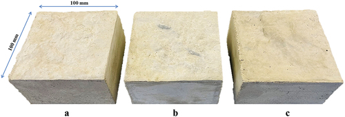
These datasets were then used to reproduce the three surfaces using cement-based grouts (water-cement ratio = 0.2), as shown in Figure 2 Flexible polyurethane resin materials were used to mould the surfaces, and 3D-printed frames were used to cast the specimens to ensure sufficient surface profile accuracy. The manufactured surface roughnesses were then verified by shear tests and back-calculating their JRCs [8].

Figure 2. (a) Smooth, (b) intermediate, (c) rough surface specimens.

2.2. Data collection

Different methods, as explained below, were used to acquire images from the grout specimen surfaces and create surface point clouds, which were used to investigate the photogrammetric method’s capacity to capture surface details. The grout specimens were also re-scanned after manufacturing as they potentially lost some details during sample preparation.

2.2.1. Structured light 3D scanner

The same handheld structured light 3D scanner (EinScan Pro 2X) was employed to obtain surface data points. Table 1 shows the scanner specifications provided by the manufacturer (SHINING 3D). Structured light is a system consisting of a projector and a camera. The camera captures the light after the projector projects specific light information onto the surface of an object and the background. The position and depth information of the object is calculated based on the changes in the light signal caused by the object, which in turn recovers the entire 3D space. Each grout specimen was placed on an automatic turntable and imaged using LED as the light source. All the output data points information was synced to a laptop through a cable simultaneously (Figure 3(a)). The entire process, which encompasses both the scanning and modelling stages, typically requires approximately 90 minutes to complete for each specimen.

Figure 3. Setup of (a) structured light 3D scanner, (b) iPhone 12 Pro Max, (c) terrestrial LiDAR scanner.

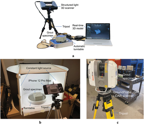
Table 1. The specifications of the structured light 3D scanner.

Scanning parameters	Specifications
Scan accuracy	.04 mm (single shot)
Scan speed	Single scan < 1s
Point distance	.16 mm
Single scan range	150 × 120 mm − 250 × 200 mm
Depth of field	100 mm
Working distance	400 mm
Light source	LED

2.2.2. Terrestrial LiDAR scanner

LiDAR scanners on portable devices, such as Apple iPhone 12 Pro Max smartphone, can scan large objects and generate rough textures. However, the specifications and performances of these LiDAR sensors are lower than survey-grade LiDAR tools in terms of resolution, i.e. points per square metre, maximum operational range, or noise characteristics [28]. No official technical specifications related to iPhone’s LiDAR sensor have been released by Apple. However, several scholars pointed out that the point cloud generated by iPhone/iPad has centimetric accuracy [42,43]. Therefore, the LiDAR on Apple iPhone 12 Pro Max cannot achieve the millimetre-level accuracy required for small objects, such as 100 mm × 100 mm specimens used in this study.

An industrial-grade TLS was used to acquire the point cloud data of grout specimens. The scanner can detect rock and ground support movements with an accuracy of 0.4 mm and is commonly used for underground monitoring [44]. It obtains high-density point cloud data in near real-time. The scanner was installed on a tripod (Figure 3(c)), and the minimum distance between the objects and the scanner was 0.5 m.

2.2.3. Portable device photogrammetry

The advances in photographic technology have enabled photogrammetry with portable devices equipped with high-resolution cameras, such as smartphones. Apple iPhone 12 Pro Max smartphone, with a 12 megapixels camera released in 2020, was used in this study as a portable photogrammetry device. Because the iPhone 12 Pro Max’s flash cannot provide a stable continuous light source, the entire photographic measurement process was carried out in a dark room with two stable light sources on both sides of the specimen.

The images taken from several different perspectives are used to reconstruct 3D models using Polycam (Polycam Inc.) software, which requires a minimum of 20 images from different perspectives and then upload to the cloud platform to reconstruct a 3D model. Polycam currently offers four different modes for users to choose from. In the Polycam application, users cannot adjust the focal length or specify a focus point as they would in the system camera. Only 1× and 2.5× focal lengths are available for selection. After securing the iPhone on a tripod, the angle and the distance between the camera and the specimen were adjusted to achieve a clear image on the screen. The turntable was rotated to capture images of the specimen from different angles. The software applies the SfM algorithm to overlapped close-range images to generate the 3D model of specimens [45]. The time needed to create the 3D model depends on the number of images and the size of the objects. It can regenerate a 3D model from 20 images within 1 minute. In cases where a larger number of images, say 250, are captured from various angles and positions, it can reconstruct a highly-detailed 3D model in less than 15 minutes. The generated model is not only the actual scale but also is located in a coordinate whose original point is the same as the object’s centre. A set of point cloud data and mesh files were exported directly from the model for further processing and analysis.

In the setup of portable device photogrammetry, the specimen was placed at the centre of the turntable. Similar to the 3D optical scanning process, the iPhone 12 Pro Max was fixed on a tripod to avoid the impact of shaking. The ‘photo’ mode and ‘manual’ shooting were selected in the Polycam application. The initial focal length was set to 2.5×, the initial shooting angle was set to 45°, and the distance between the camera and the sample was 300 mm (Figure 3(b)). After setting up the shooting parameters, the images were captured while rotating the turntable. A total of 120 photos were taken in this round of shooting. Then, the shooting angle was adjusted to 30, 60, and 75 degrees gradually, and another complete round of images was taken at each angle. A total of 250 images were captured for each specimen during the image acquisition process. Next, the ‘upload and processing’ step was entered, with the ‘Raw’ detail and ‘Use Object Masking’ options being checked. The ‘Upload & Process’ button was clicked to commence the 3D model reconstruction. The reconstruction process took approximately 15 minutes. The point cloud data of the reconstructed model was directly exported to CloudCompare for further processing.

2.3. Assessment of photogrammetric measurement accuracy

The 3D point cloud models generated by different scanning methods were processed to extract only the specimen surfaces for roughness quantification analysis. Three parameters, multiscale model-to-model cloud comparison (M3C2) [38], JRC, and the 3D roughness parameter [46] were used to evaluate the accuracy of the photogrammetry method. The open-source FSAT toolbox [17] was applied as a computation method to calculate the JRC and 3D roughness parameter from the point cloud data of the specimen surfaces. This method loads the raw irregular point cloud data and regenerates a uniform mesh grid with height information. Surfaces are split in different directions and disassembled in single profiles to calculate roughness parameters. The 2D line profiles extracted from the meshed point clouds were plotted and compared. Shear tests were conducted to back-calculate the JRC in the shear direction to quantify the surface roughness physically. Considering the model reconstructed by a structured light 3D scanner as the benchmark, the M3C2 distances between the structured light 3D scanner and smartphone photogrammetry models were calculated. The distance distributions mostly followed a normal distribution and were used to evaluate the accuracy of the portable device photogrammetric model.

2.3.1. M3C2

Lague et al. [38] introduced M3C2 for point cloud comparison in 3D, which is included in the CloudCompare open-source software (www.danielgm.net/cc). Compared with traditional distance calculation algorithms that calculate the nearest neighbour point distance, the M3C2 algorithm was developed to calculate the orthogonal distance between two point clouds in 3D, which avoids meshing steps and mitigates the impact of point uncertainty. At its core, the M3C2 algorithm compares corresponding points between two point cloud models and quantifies the geometric differences. It operates by dividing the point clouds into smaller local patches and calculating the optimal transformation that aligns each patch to its corresponding patch in the reference model.

In the M3C2 method, in the reference point cloud, the given core point j is the centre of the sphere, the normal scale D is the diameter, and ${\vec{N}}_j$is the normal vector of the fitted plane for all points in the sphere. The normal vector is oriented positively to the compared point cloud. Then, the normal vector is used to project j onto each point cloud at a projection scale d that defines the average positions of each cloud in the vicinity of the core point. A cylinder of diameter d whose axis goes through j and along the normal vector is created. Two point subsets are generated at the intersection of each cloud with the cylinder. Projecting each subset on the cylinder’s axis gives two distributions of distances. The average positions $j_1,j_2$ of each cloud are the mean of the distribution, and the standard deviations present the estimation of point cloud roughness. Finally, the local distance between the two clouds is the distance between $j_1$ and $j_2$ [7,38]. By analysing the differences in local distance, the algorithm produces a colour-coded map that represents the spatial deviations between the point clouds. The resulting map provides valuable information about the overall alignment and registration quality of the point clouds. Regions with significant deviations are visualised with distinct colours, making it easy to identify areas of discrepancy or potential errors in the data.

2.3.2. JRC

The statistical parameter $Z_2$ was computed for JRC analysis in this study. It is used to numerically calculate the JRC from the line profiles and avoid the subjectivity of JRC estimation [12]. $Z_2$ is highly sensitive to the sampling interval, and different empirical equations are used to calculate JRC for different sampling intervals. In this study, a sampling interval of 0.1 mm was adopted to $Z_2$ and JRC calculation. The related equation was proposed by Jang et al. [47].

(1) $Z_2={\left[\frac{1}{M{(Dx)}^2}\sum _{i=1}^M{\left(y_{i+1}-y_i\right)}^2\right]}^{\frac{1}{2}}$(1)

(2) $JRC=54.47\times Z_{2}0.394-19.13$(2)

where $M$ is the number of intervals along the profile length, $Dx$ is the point interval and $\mathrm{\Delta }y=y_{i+1}-y_i$, is the difference between two adjacent points.

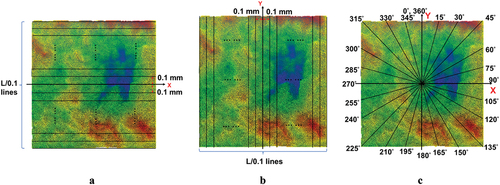
The point intervals of the structured light 3D scanner and portable device photogrammetry models were not uniform. The point cloud data was thus reassembled with a fixed interval of 0.1 mm. A matrix was generated to save the height information of points. The matrix size varied depending on the analysed surface dimension and specified interval. Missing data points caused by surface extraction were eliminated by replacing them with not a number (NaN), especially in the edge sections. The 2D profiles were extracted at 0.1 mm spacing from each model in X and Y directions. Then, the JRC of each profile was calculated using Equations (1) and (2). The anisotropic characteristics of the JRC were accounted for by calculating JRC in different directions, as shown in Figure 4. The average value of JRC was considered to represent the whole surface roughness.

Figure 4. Profiles selected on the smooth surface with a sampling interval of 0.1 mm, (a) X direction, (b) Y direction, (c) different directions were selected at the interval of 15°.

For JRC back-calculation, shear tests were conducted along the Y-axis direction on the grout specimens, and sister grout specimens were prepared for the compressive and plane shear test to obtain the unconfined compressive strength (UCS) and basic friction angle, ${\phi }_b$. Specimens preparation and all experimental procedures complied with the Australian Standard AS 1012. The empirical relationship between peak shear strength and JRC is described by [48]:

(3) $\tau ={\sigma }_n\cdot tan\left[JRC\cdot lo{g}_{10}(JCS/{\sigma }_n)+{\phi }_b\right]$(3)

hence the JRC can be back-calculated by:

(4) $JRC=\frac{\text{arctan}\frac{\tau }{{\sigma }_n}-{\phi }_b}{lo{g}_{10}(JCS/{\sigma }_n)}$(4)

where $\tau$ is peak shear strength, ${\sigma }_n$ is effective normal stress, $JCS$ is joint wall compressive strength, which can be considered UCS for unweathered joints [8].

The JRC error, which was used to assess the capacity of the photogrammetry method in JRC estimation [7], is defined as:

(5) $\begin{array}{c}erro{r}_{JRC}=\frac{JR{C}_2-JR{C}_1}{JR{C}_1}\\ \end{array}$(5)

where $JR{C}_1$ is the benchmark, calculated from the structured light 3D scanner model and $JR{C}_2$ is obtained from the portable device photogrammetry model.

2.3.3. 3D roughness parameter

During shear under low normal stress, the morphology of the fracture surface is considered the most significant geometrical boundary [17]. Grasselli [46] proposed a 3D roughness parameter to quantify the morphology of the 3D surface, which Tatone and Grasselli [14] later improved. The shear resistance is mainly developed by the areas facing the shear direction, and a steeper contact area develops stronger resistance. Grasselli [46] used the apparent dip angle to describe the activated area during shearing and extended it to a 3D triangulated unregular surface. Each triangle $i$ is expressed by its normal vector ${\vec{n}}_i$, and the projection of ${\vec{n}}_i$ on horizontal shear surface is ${\vec{n}}_{i0}$. The dip angle of each triangle ${\theta }_i$ can be calculated as:

(6) $cos{\theta }_i=\frac{{\overrightarrow{n}}_i{\overrightarrow{n}}_{i0}}{\left|{\overrightarrow{n}}_i\right|\left|{\overrightarrow{n}}_{i0}\right|}$(6)

For different shear direction $\vec{s}$, the azimuth ${\alpha }_i$ can be calculated as [49]:

(7) $\begin{array}{c}cos{\alpha }_i=\frac{\vec{s}{\vec{n}}_{i0}}{\left|\vec{s}\right|\left|{\vec{n}}_{i0}\right|}\\ \end{array}$(7)

The apparent dip of each triangle ${\theta }_i^{\ast }$ under shear direction $\vec{s}$ can be described as:

(8) $tan{\theta }_i^{*}=-cos{\alpha }_i\cdot tan{\theta }_i$(8)

A maximum apparent dip ${\theta }_{max}^{\ast }$ can be found from all triangles on the surface. The requirement $tan{\theta }_i^{\ast }>0$ can filter out the triangles facing the shear direction. The maximum possible contact area $A_0$ and potential contact area $A_{{\theta }^{\ast }}$ for threshold inclination ${\theta }^{\ast }$ have the empirical relationship expressed as:

(9) $A_{\theta *}=A_0\left(\frac{{\theta }_{max}^{*}-\theta *}{{\theta }_{max}^{*}}\right)C$(9)

where $C$ is the empirical roughness coefficient [46]. The 3D roughness parameter in the form of ${\theta }_{max}^{\ast }/\left(C+1\right)$ [14] has been widely used to measure roughness [49–51]. The Delaunay triangulation, a commonly used method to obtain a closed surface from discrete points [17,50], was used in this study. In this method, each point connects to adjacent points, so that generated triangle does not overlap with the others. The sampling interval affects the ${\theta }_{max}^{\ast }/{\left(C+1\right)}_{2D}$ proposed by Tatone and Grasselli [14], however, its impact on the ${\theta }_{max}^{\ast }/{\left(C+1\right)}_{3D}$ is currently unclear. Therefore, a sampling interval of 0.2 mm, as used by Chen et al [52,53], was employed to investigate the 3D roughness parameter in this study.

3. Results and analysis

3.1. Reconstructed 3D surface models

Three reconstructed 3D models were obtained from each surface by (i) the structured light 3D scanner (the benchmark), (ii) the portable device photogrammetry, and (iii) the terrestrial LiDAR scanner. Only the surface part of each specimen was retained for analyses and comparisons. Figure 5 illustrates the topography of the reconstructed models. Table 2 provides the details of the reconstructed surface models. It shows that the total number of points and average point density of the TLS is considerably lower than the other two methods. The TLS’s topography neither accurately represents the surface roughness (Figure 5(c)) nor can it be used to quantify the roughness precisely due to the scattering of points and difficulties in removing its noises.

Figure 5. The reconstructed 3D surfaces from (a) structured light 3D scanner, (b) portable device photogrammetry, (c) terrestrial LiDAR scanner.

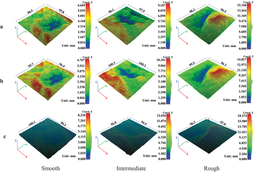
Table 2. Information of reconstructed 3D surface models.

Scanning Method	Surface Roughness	Size			Number of Points	Average Point Density (points/mm^2)
		X (mm)	Y (mm)	Z (mm)
Structured light 3D scanner	Smooth	95.8	98.5	6.7	198,553	21
	Intermediate	97.9	98.3	9.2	193,919	20
	Rough	96.5	98.3	15.2	205,183	21
Portable device photogrammetry	Smooth	96.4	99.7	6.8	372,694	38
	Intermediate	100.3	100.4	10.4	508,993	50
	Rough	96.3	99.5	14.8	474,086	49
Terrestrial LiDAR scanner	Smooth	96.2	100.1	8.2	28,454	3
	Intermediate	6.0	94.4	12.7	24,251	3
	Rough	97.0	96.3	18.3	25,722	3

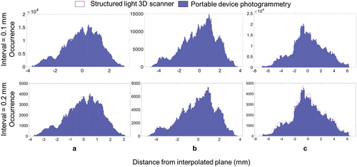
A uniformly distributed grid surface and a fitted plane by interpolating points were generated from the point clouds. As mentioned in section 2.3, line profile data extraction and point interval spacing were set to 0.1 mm for JRC calculation and 0.2 mm for 3D roughness parameter calculation. The height information of points was stored in a matrix. The distribution of distances from the generated grid points to the interpolated plane is shown in Figure 6.

Figure 6. The distance distribution from generated grid points to the interpolated (a) smooth, (b) intermediate, (c) rough surface (relative height).

The initial assessment of the point cloud data indicated that the TLS’s results failed to meet expectations in this study because the TLS produced a point cloud that was an order of magnitude less dense than the other two methods and contained many noise points. Its sparse point clouds could not be used for high-accuracy mesh generation and quantification of surface roughness. Low-density point clouds could not retain sufficient details to produce surface triangulation. This is because the TLS used in this experiment was designed for relatively large-scale industrial applications and could not provide satisfactory results for lab-scale specimens. Portable photogrammetric devices, such as iPhone 12 Pro Max used in this study, and structured light 3D scanners provide more data points and details at this scale, as presented in Table 2.

Scanning dark (black) objects is challenging for the structured light 3D scanner because the black colour does not reflect light to the sensors. In this study, the grey colour of the specimens and constant indoor light sources highly assisted in scanning the surface. Fixing the scanner avoided errors caused by vibration when operated by hand. These measures ensure accuracy but limit their potential for field-scale applications. Rocks are heterogeneous with different colours and maintaining light constantly in practice is not readily achievable, especially in underground excavation engineering. Data transfer and supplying power are other challenges associated with structured light 3D scanners. As shown in Figure 6 and Table 2, portable photogrammetric devices, such as smartphones used in this study, can capture roughness details of lab-scale specimens with relatively comparable accuracy to structured scanners by obtaining images at close distances. The light source requirements of such portable photogrammetric devices are not as limiting as optical scanners. Although no attempts have been made to scan and analyse large-scale rock surfaces with portable photogrammetric devices here, their portability, affordability, and demonstrated accuracy at the lab scale show their potential for industrial applications.

3.2. Comparison and assessment

Figure 7 shows the distribution and occurrence of cloud-to-cloud distance (M3C2) between benchmark and photogrammetry point clouds for each surface. The difference significantly appears at the surface’s edge, and the height difference at the centre is not apparent. The occurrences were fitted into a normal distribution, and their means, standard deviations, and root mean square error (RMSE) were obtained (Table 3). The accuracy of the portable device photogrammetry model is represented by RMSE [54]. As noted, TLS could not provide high-quality data for lab-scale specimens, so TLS’s data were not used for further analysis. Although the same capturing and scanning methods were employed for each roughness specimen, the M3C2 results for the reconstructed surface varied, indicating that the texture of the specimens influences the accuracy of reconstructed 3D models An et al. [7].

Figure 7. Distribution and occurrence of the cloud-to-cloud distance of the point clouds, (a) smooth, (b) intermediate, (c) rough surface.

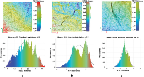
Table 3. The cloud-to-cloud distance between the structured light 3D scanner model and the portable device photogrammetry model.

	Mean (mm)	Standard deviation (mm)	RMSE (mm)
Smooth	0.30	0.59	0.66
Intermediate	0.32	0.72	0.79
Rough	−0.34	0.51	0.62

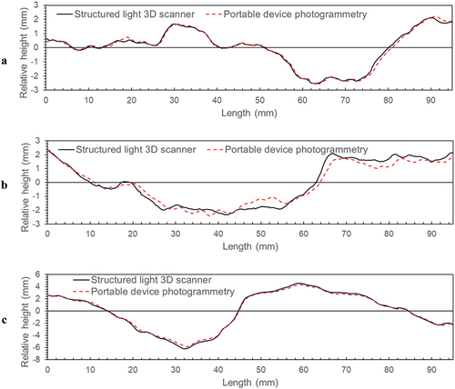
The 3D surfaces can theoretically yield a profile at any position on the surface for computational analysis. Figure 8 demonstrates line profile comparisons along the X-axis centre line of the three different roughness models constructed by the structured light 3D scanner and portable device photogrammetry.

Figure 8. Comparison of the line profiles from the structured light 3D scanner and portable device photogrammetry images at the surface centre along the X-axis. a smooth, b intermediate, and c rough surface.

The interval and height information of each line profile $\left(L_1\right)$ was extracted, and the $Z_2$ parameter and JRC of each profile were calculated by Equations (1) - (2). The JRC of the entire surface along the X and Y directions were then computed by averaging the JRC of line profiles parallel to $L_1$, which were spaced at 0.1 mm intervals (Figure 4(a,b)), and the results are provided in Table 4. Considering the anisotropic characteristics of JRC, a polar coordinate system was established with the centre of the surface, and line profiles were extracted at 15° intervals (Figure 4(c)). Similarly, their average value was calculated as the JRC of the whole surface [15,17,55]. The results are shown in Table 4, and Figure 9 shows the anisotropic distributions of JRC for different surfaces.

Figure 9. Anisotropic distribution of average JRC values for (a) smooth, (b) intermediate, and (c) rough surface.

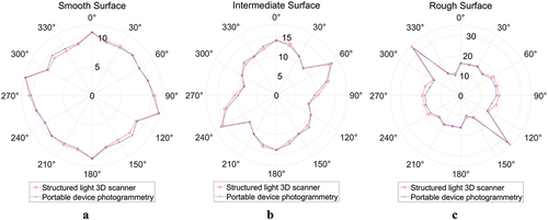
Table 4. Comparison of JRC values for different surfaces.

Surface	Direction	Structured light 3D scanner		Portable device photogrammetry	ErrorJRC	Back-calculated JRC
Smooth	X		9.50	9.33	−1.79%
	Y		8.82	8.66	−1.81%	9.58
	Anisotropy		9.71	9.77	0.62%
Intermediate	X		10.78	11.12	3.15%
	Y		11.73	11.48	−2.19%	11.10
	Anisotropy		11.83	12.10	2.28%
Rough	X		17.43	16.40	−5.92%
	Y		12.39	11.97	−3.42%	\
	Anisotropy		17.66	16.90	−4.31%

Six UCS tests and two plane shear tests were conducted on the sister specimens. The UCS of the grout specimen was 42.73 MPa and ${\phi }_b$ was 34.35°. Table 4 also provides the average of JRC back-calculated from the shear tests using equation (4). The shear direction was the same as the positive direction of the Y-axis. The experimental JRC of the rough surface could not be obtained because there was a large area of height difference in the centre of the rough specimens that interlocked during the shear test leading to inaccurate experimental results. The considerable height difference also can be observed in Figures 5 and 9, where the JRC of the 135°-315° profile is over 20.

An et al. [7] indicated that the SfM photogrammetry tends to underestimate the JRC of the rock joint surfaces, however, this circumstance did not occur in this study. For all three surfaces in this study, the entire surface JRC along the X- and Y-axis directions were smaller than the average anisotropic JRC of the entire surface. Because when calculating the JRC for the entire surface, the surface undulations in other directions may be more prominent. The profiles have the most significant fluctuations along 105–285° direction for the smooth surface. The largest waviness occurs at 60–240° for the intermediate surface and 135–315° for the rough surface. Minor differences were observed in the JRC values calculated from portable device photogrammetry models and the benchmark structured light 3D models and back-calculated JRC values. However, the JRC values were in the same range, with almost less than 5% in most cases. This again demonstrates the extraordinary capacity of portable device photogrammetry, smartphones, in capturing the roughness details.

Furthermore, the 3D roughness parameter ${\theta }_{max}^{\hspace{0.17em}}/\left(C+1\right)$ proposed by Tatone and Grasselli [14], which represents the topography of surfaces, was calculated for each surface (Figure 10). Table 5 and Figure 10 show that portable device photogrammetry could achieve fairly consistent results with benchmark data. The distribution shape of the smooth surface approximates a circle, indicating that the undulations are about the same in each direction. The data distribution on intermediate and rough surfaces is approximately elliptical, with the major axis along the Y- and X-axes, respectively. It indicates that the intermediate surface has a relatively higher undulation along the Y-axis than on the X-axis. The rough surface has a relatively higher undulation along the X-axis. These are consistent with the constructed 3D surfaces shown in Figure 5.

Figure 10. Distribution of 3D roughness parameter for a smooth, b intermediate, and c rough surface.

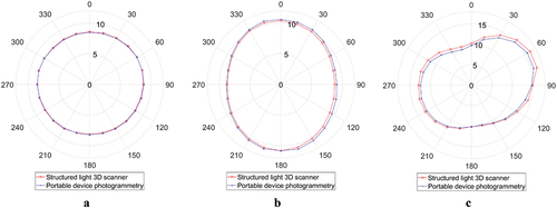
Table 5. Comparison of 3D roughness parameter $\frac{{\theta }_{max}^{\ast }}{C+1}$.

Surface	Structured light 3D scanner	Portable device photogrammetry	$Erro{r}_{\frac{{\theta }_{max}^{\ast }}{C+1}}$
Smooth	8.51	8.50	−0.12%
Intermediate	9.66	9.90	2.48%
Rough	12.53	12.05	−3.83%

4. Discussion

Overall slight differences were found by comparing the M3C2 distance, JRC, and the 3D roughness parameter of the reconstructed surfaces from portable device photogrammetry and the benchmark data. These minor differences or errors could have occurred during the imaging and surface digitalisation. After comparing multiple smartphones and different shooting angles, An et al. [7] also concluded that the accuracy of surface reconstruction using smartphone photogrammetry is comparable to that of 3D laser scanners for laboratory-sized surfaces. It is still worth noting that more joint surfaces, more types of rock, more lighting conditions, and scale effects should be considered for further verification of the applicability of portable device photogrammetry in future.

The shooting angle and the light source can cause the object to appear in shadow in some areas. Although the specimens were grey and indoor consistent light was used for imaging, there could still be the possibility of some dark regions to which the structured light scanner is not sensitive, which could cause errors. Further research is needed to investigate the influence of specular reflection on smartphone photogrammetric measurements caused by smooth-textured rocks or rock joints in the presence of liquids. The requirements of light intensity for different textured rocks need to be tested, which can be quantitatively expressed by lux and measured by luminance metres.

The camera’s specifications, such as resolution and focal length, can lead to various photogrammetric measurement results. Higher resolution generally provides greater detail and accuracy with larger file sizes, and higher computational resource requirements. A longer focal length narrows the field of view and can result in a higher level of detail for objects located at a distance. On the other hand, a shorter focal length provides a wider field of view but may result in reduced detail for distant objects. When applying this technique to large-scale rock masses in engineering, theoretically, a shorter focal length should be used to capture the overall topography, while a longer focal length should be used to capture local details. However, optimal operation guidelines need to be established in further research.

While the Polycam application is capable of reconstructing high-precision 3D models within 15 minutes, its efficiency relies on cloud computing. This means that during the reconstruction process, the smartphone must be connected to the internet to upload the images to the cloud for model reconstruction. In the process of surface digitisation, the analysed surfaces were extracted from the entire 3D models. Due to a large amount of noise at the model’s edges, the extraction process resulted in different dimensions of the analysed surfaces. The value of normal scale $D$ and projection scale $D$ have an impact on the surface normal orientation for M3C2 distance calculations [38]. Some pre-set parameters in the FSAT toolbox can cause errors. For example, the grid spacing chosen impacts the density of the point cloud. Larger grid spacing means a sparse rebuilt mesh with less height information stored. When selecting the grid spacing, consideration should be given to the density of the original point cloud. Using a small grid spacing on a sparse point cloud can result in a large number of random points, and their elevation information may not align with the actual measurement results. On the other hand, using a large grid spacing on a dense point cloud can lead to the loss of valuable point cloud data, thereby reducing measurement accuracy. Variation in grid spacing consequently changes $Z_2$, JRC and 3D roughness parameters.

5. Conclusion

Despite the wide range of techniques available for digitising rock surfaces, a reliable technique that strikes a balance between accuracy, cost-effectiveness, and efficiency does not still exist. The utilisation of a smartphone equipped with a high-quality lens and powerful processor offers a cost-effective solution for photogrammetric applications. To evaluate the feasibility of portable device photogrammetry for digitising rock surface roughness, three different scanning devices, a structured light 3D scanner, a smartphone, and a TLS, were used to scan lab-scale grout specimens with different surface roughness.

The results showed that the density of the point cloud obtained by the TLS was much lower than the other two methods, whose results contain lots of noise points that needed to be removed manually. This lack of point density hindered further quantitative surface roughness analysis. The mean cloud-to-cloud distance was determined using the M3C2 algorithm and compared with the point clouds generated by a structured light 3D scanner and a portable photogrammetry device, which showed that the mean distances were 0.30 mm, 0.32 mm, and −0.34 mm for smooth, intermediate, and rough surfaces, respectively. The open-sourced FSAT toolbox was employed to calculate the reconstructed surfaces’ JRC and 3D roughness parameters. The errors of JRC and 3D roughness parameter generally increased with the surface roughness but were less than 5%, except for the JRC of the rough surface along the X-axis direction.

Overall, the results suggest that portable device photogrammetry technology can produce relatively reliable estimations of JRC and Grasselli’s 3D roughness parameter for the three different surfaces used in this study, comparable to structured light 3D scanners. The smartphones’ high-quality lenses produce high-resolution images, and their advanced processors allow for processing images and reconstructing 3D models faster than most laser scanners, a highly-detailed 3D model for lab-scale specimen can be constructed within 15 minutes. The smartphones’ cost-effectiveness, portability, and efficiency make them a viable alternative to traditional photogrammetry systems with the potential for industrial application to large rock joint surfaces. However, for applying photogrammetry to measure roughness on a large scale, limitations and potential variations in scale that may arise due to the device’s technical specifications, such as the resolution and focal length, need to be considered. Assessing the suitability of the length represented by single pixel point in calculating roughness is necessary. Therefore, future studies to assess their feasibility in industrial applications are recommended.

Acknowledgments

The work was supported by the Australian Coal Industry Research Program (ACARP) under Grant C29025. Special thanks to Mr Kanchana Gamage, Mr Mark Whelan, and Mr Gabriel Graterol Nisi from UNSW Sydney for their assistance in laboratory tests.

Disclosure statement

No potential conflict of interest was reported by the author(s).

Additional information

Funding

The work was supported by the Australian Coal Industry’s Research Program [C29025].

References

- J.P. Monticeli Roughness characterization of discontinuity sets by profilometer and scanner images, ISRM Regional Symposium-8th South American Congress on Rock Mechanics, Buenos Aires, Argentina, OnePetro, 2015.
- V.P. Cantarella, JRC estimation with 3D laser scanner images – SBMR 2016, Brazilian Symposium on Rock Mechanics, Belo Horizonte, Minas Gerais, Brazil, 2016.
- N. Fardin, Q. Feng, and O. Stephansson, Application of a new in situ 3D laser scanner to study the scale effect on the rock joint surface roughness, Int. J. Rock Mech. Min. 41 (2) (2004), pp. 329–335. https://doi.org/10.1016/S1365-1609(03)00111-4.
- G. Luetzenburg, A. Kroon, and A.A. Bjørk, Evaluation of the Apple iPhone 12 Pro LiDAR for an application in geosciences, Sci. Rep. 11 (1) (2021), pp. 22221. https://doi.org/10.1038/s41598-021-01763-9.
- Y.A. Asmare, L.D. Stetler, and Z.J. Hladysz, A New Method for Estimating 3D Rock Discontinuity Roughness from a Terrestrial LiDAR Data using Slope Angles of Triangular Facets, 48th U.S. Rock Mechanics/Geomechanics Symposium, Minneapolis, Minnesota, United States, 2014.
- J. Sirkiä, Photogrammetric calculation of JRC for rock slope support design, Proceedings of the 8th International Symposium on Ground Support in Mining and Underground Construction, Luleå, Sweden, 2016.
- P. An, K. Fang, Q. Jiang, H. Zhang, and Y. Zhang, et al., Measurement of rock joint surfaces by using smartphone structure from motion (SfM) photogrammetry, sensors 21 (3) (2021), pp. 922. https://doi.org/10.3390/s21030922.
- N.B.V. choubey, The Shear Strength of Rock Joints in Theory and Practice, Rock Mech. 10 (1–2) (1977), pp. 1–54. https://doi.org/10.1007/BF01261801.
- A.J. Beer and J.S. Coggan, Technical note estimation of the joint roughness coefficient (JRC) by visual comparison, Rock Mech. Rock Eng 35 (1) (2002), pp. 65–74. https://doi.org/10.1007/s006030200009.
- G. Weissbach, A new method for the determination of the roughness of rock joints in the laboratory, Int. J. Rock Mech. Rock Eng 15 (3) (1978), pp. 131–133. https://doi.org/10.1016/0148-9062(78)90007-4.
- P. Alameda-Hernández, J. Jiménez-Perálvarez, J.A. Palenzuela, R. El Hamdouni, C. Irigaray, M.A. Cabrerizo, and J. Chacón, Improvement of the JRC calculation using different parameters obtained through a new survey method applied to rock discontinuities, Rock Mech. Rock Eng 47 (6) (2014), pp. 2047–2060. https://doi.org/10.1007/s00603-013-0532-2.
- R. Tse and D. Cruden, Estimating joint roughness coefficients, Int. J. Rock Mech. Min. Sci. Geomech. Abstr. 16 (5) (1979), pp. 303–307. Elsevier. https://doi.org/10.1016/0148-9062(79)90241-9.
- N.H. Maerz, J.A. Franklin, and C.P. Bennett, Joint roughness measurement using shadow profilometry, Int. J. Rock Mech. Min. Sci. Geomech. Abstr. 27 (5) (1990), pp. 329–343. Elsevier. https://doi.org/10.1016/0148-9062(90)92708-M.
- B.S. Tatone and G. Grasselli, A new 2D discontinuity roughness parameter and its correlation with JRC, Int. J. Rock Mech. Min. Sci. 47 (8) (2010), pp. 1391–1400. https://doi.org/10.1016/j.ijrmms.2010.06.006.
- H. Bao, Geometrical heterogeneity of the joint roughness coefficient revealed by 3D laser scanning, Eng. Geol. 265 (2020), pp. 105415. https://doi.org/10.1016/j.enggeo.2019.105415.
- C.-C. Xia, New Peak Shear Strength Criterion of Rock Joints Based on Quantified Surface Description, Rock Mech. Rock Eng. 47 (2) (2013), pp. 387–400. https://doi.org/10.1007/s00603-013-0395-6.
- T. Heinze, S. Frank, and S. Wohnlich, FSAT – A fracture surface analysis toolbox in MATLAB to compare 2D and 3D surface measures, Comput. Geotech. 132 (2021), pp. 103997. https://doi.org/10.1016/j.compgeo.2020.103997.
- G. Grasselli, P. Egger, Constitutive law for the shear strength of rock joints based on three-dimensional surface parameters, Int. J. Rock Mech. Min. Sci. 40 (1)(2003), pp. 25–40. https://doi.org/10.1016/S1365-1609(02)00101-6.
- B.S. Tatone, Quantitative Characterization of Natural Rock Discontinuity Roughness In-situ and in the Laboratory, University of Toronto, Toronto, Canada, 2009.
- Q. Jiang, B. Yang, F. Yan, C. Liu, Y. Shi, L. Li, New Method for Characterizing the Shear Damage of Natural Rock Joint Based on 3D Engraving and 3D Scanning, Int. J. Geomech. 20 (2), (2020), https://doi.org/10.1061/(ASCE)GM.1943-5622.0001575.
- Q. Jiang, Y. Yang, F. Yan, J. Zhou, S. Li, B. Yang, and H. Zheng, et al., Deformation and failure behaviours of rock-concrete interfaces with natural morphology under shear testing, Constr. Build. Mater. 293 (2021), pp. 123468. https://doi.org/10.1016/j.conbuildmat.2021.123468.
- J.D. Aubertin and D.J. Hutchinson, Scale-dependent rock surface characterization using LiDAR surveys, Eng. Geol. 301 (2022), pp. 301. https://doi.org/10.1016/j.enggeo.2022.106614.
- M. Lato, M.S. Diederichs, D.J. Hutchinson, and R. Harrap, et al., Optimization of LiDAR scanning and processing for automated structural evaluation of discontinuities in rockmasses, Int. J. Rock Mech. Min. Sci. 46 (1) (2009), pp. 194–199. https://doi.org/10.1016/j.ijrmms.2008.04.007.
- M.J. Westoby, S.A. Dunning, J. Woodward, A.S. Hein, S.M. Marrero, K. Winter, and D.E. Sugden, Interannual surface evolution of an Antarctic blue-ice moraine using multi-temporal DEMs, Earth Surf. Dynam. 4 (2) (2016), pp. 515–529. https://doi.org/10.5194/esurf-4-515-2016.
- K. Kingsland, Comparative analysis of digital photogrammetry software for cultural heritage, Digit. Appl. Archaeol. Cult. Heritage 18 (2020), pp. e00157. https://doi.org/10.1016/j.daach.2020.e00157.
- Y. Han, S. Wang, D. Gong, Y. Wang, Y. Wang, and X. Ma, State of the art in digital surface modelling from multi-view high-resolution satellite images, ISPRS Ann. Photogramm. Remote Sens. Spatial Inf. Sci. 2 (2020), pp. 351–356. https://doi.org/10.5194/isprs-annals-V-2-2020-351-2020.
- A. Corradetti, T. Seers, M. Mercuri, C. Calligaris, A. Busetti, and L. Zini, et al., Benchmarking different SfM-MVS photogrammetric and iOS LiDAR acquisition methods for the digital preservation of a short-lived excavation: A case study from an area of sinkhole related subsidence, Remote Sens. 14 (20) (2022), pp. 5187. https://doi.org/10.3390/rs14205187.
- S. Tavani, A. Billi, A. Corradetti, M. Mercuri, A. Bosman, M. Cuffaro, T. Seers, and E. Carminati, et al., Smartphone assisted fieldwork: Towards the digital transition of geoscience fieldwork using LiDAR-equipped iPhones, Earth-Sci. Rev. 227 (2022), pp. 2022. 227. https://doi.org/10.1016/j.earscirev.2022.103969.
- N. Micheletti, J.H. Chandler, and S.N. Lane, Investigating the geomorphological potential of freely available and accessible structure‐from‐motion photogrammetry using a smartphone, Earth Surf. Process. Landforms 40 (4) (2015), pp. 473–486. https://doi.org/10.1002/esp.3648.
- M. Jaud, M. Kervot, C. Delacourt, and S. Bertin, et al., Potential of smartphone SfM photogrammetry to measure coastal morphodynamics, Remote Sens. 11 (19) (2019), pp. 2242. https://doi.org/10.3390/rs11192242.
- P. An, K. Fang, Y. Zhang, Y. Jiang, and Y. Yang, et al., Assessment of the trueness and precision of smartphone photogrammetry for rock joint roughness measurement, measurement 188 (2022), pp. 110598. https://doi.org/10.1016/j.measurement.2021.110598.
- K. Fang, J. Zhang, H. Tang, X. Hu, H. Yuan, X. Wang, P. An, and B. Ding, et al., A quick and low-cost smartphone photogrammetry method for obtaining 3D particle size and shape, Eng. Geol. 322 (2023), pp. 107170. https://doi.org/10.1016/j.enggeo.2023.107170.
- K. Fang, P. An, H. Tang, J. Tu, S. Jia, M. Miao, and A. Dong, et al., Application of a multi-smartphone measurement system in slope model tests, Eng. Geol. 295 (2021), pp. 106424. https://doi.org/10.1016/j.enggeo.2021.106424.
- K. Fang et al, Comprehensive assessment of the performance of a multismartphone measurement system for landslide model test, Landslides. 20 (2023), pp. 845–864. https://doi.org/10.1007/s10346-022-02009-z.
- R.N. Gillihan. Accuracy Comparisons of iPhone 12 Pro LiDAR Outputs, University of Colorado, Denver, CO, United States, 2021.
- Y. Ge, K. Chen, G. Liu, Y. Zhang, and H. Tang, et al., A low-cost approach for the estimation of rock joint roughness using photogrammetry, Eng. Geol. 305 (2022), pp. 106726. https://doi.org/10.1016/j.enggeo.2022.106726.
- A. Paixão, J. Muralha, R. Resende, and E. Fortunato, Close-range photogrammetry for 3D rock joint roughness evaluation, Rock Mech. Rock Eng 55 (6) (2022), pp. 3213–3233. https://doi.org/10.1007/s00603-022-02789-9.
- D. Lague, N. Brodu, and J. Leroux, Accurate 3D comparison of complex topography with terrestrial laser scanner: Application to the Rangitikei canyon (NZ), ISPRS J. Photogramm. Remote Sens. 82 (2013), pp. 10–26. https://doi.org/10.1016/j.isprsjprs.2013.04.009.
- V. Zahs, L. Winiwarter, K. Anders, J.G. Williams, M. Rutzinger, and B. Höfle, et al., Correspondence-drivenplane-based M3C2 for lower uncertainty in 3D topographic change quantification, ISPRS J. Photogramm. Remote Sens. 183 (2022), pp. 541–559. https://doi.org/10.1016/j.isprsjprs.2021.11.018.
- A.R. Beer, J.M. Turowski, and J.W. Kirchner, Spatial patterns of erosion in a bedrock gorge, J. Geophys. Res. Earth Surf. 122 (1) (2017), pp. 191–214. https://doi.org/10.1002/2016JF003850.
- V. Zahs, M. Hämmerle, K. Anders, S. Hecht, R. Sailer, M. Rutzinger, J.G. Williams, and B. Höfle, Multi‐temporal 3D point cloud‐based quantification and analysis of geomorphological activity at an alpine rock glacier using airborne and terrestrial LiDAR, Permafr. Periglac. Process. (2019), https://doi.org/10.1002/ppp.2004.
- A. Spreafico, F. Chiabrando, L. Teppati Losè, and F. Giulio Tonolo, The ipad pro built-in lidar sensor: 3d rapid mapping tests and quality assessment, Int. Arch. Photogramm. Remote Sens. Spatial Inf. Sci. 43 (2021), pp. 63–69. https://doi.org/10.5194/isprs-archives-XLIII-B1-2021-63-2021.
- P. Chase, K. Clarke, A. Hawkes, S. Jabari, and J. Jakus, Apple IPhone 13 Pro Lidar Accuracy Assessment for Engineering Applications, Transforming Construction with Reality Capture Technologies: The Digital Reality of Tomorrow, August 23–25, 2022, Fredericton, New Brunswick, Canada, 2022. https://doi.org/10.57922/tcrc.645
- L.-P. Gelinas, Advanced geotechnical monitoring technology to assess ground support effectiveness, Ground Support 2019: Proceedings of the Ninth International Symposium on Ground Support in Mining and Underground Construction, Perth, WA, Australia, 2019. pp. 59–74. https://doi.org/10.36487/ACG_rep/1925_02_Gelinas.
- R. Eker, 3d Modelling of a Historic Windmill: Ppk-Aided Terrestrial Photogrammetry Vs Smartphone App. The International Archives of the Photogrammetry, Int. Arch. Photogramm. Remote Sens. Spatial Inf. Sci. XLIII-B2-2022 (2022), pp. 787–792. https://doi.org/10.5194/isprs-archives-XLIII-B2-2022-787-2022.
- G. Grasselli, J. Wirth, and P. Egger, Quantitative three-dimensional description of a rough surface and parameter evolution with shearing, Int. J. Rock Mech. Min. Sci. 39 (6) (2002), pp. 789–800. https://doi.org/10.1016/S1365-1609(02)00070-9.
- H.-S. Jang, S.-S. Kang, and B.-A. Jang, Determination of Joint Roughness Coefficients Using Roughness Parameters, Rock Mech. Rock Eng. 47 (6) (2014), pp. 2061–2073. https://doi.org/10.1007/s00603-013-0535-z.
- N. Barton, Review of a new shear-strength criterion for rock joints, Eng. Geol. 7 (4) (1973), pp. 287–332. https://doi.org/10.1016/0013-7952(73)90013-6.
- L. Song, Q. Jiang, L.-F. Li, C. Liu, X.-P. Liu, and J. Xiong, An enhanced index for evaluating natural joint roughness considering multiple morphological factors affecting the shear behavior, Bull. Eng. Geol. Environ 79 (4) (2020), pp. 2037–2057. https://doi.org/10.1007/s10064-019-01700-1.
- N. Babanouri and S. Karimi Nasab, Proposing Triangulation-Based Measures for Rock Fracture Roughness, Rock Mech. Rock Eng 50 (4) (2016), pp. 1055–1061. https://doi.org/10.1007/s00603-016-1139-1.
- L. Ban, W. Du, C. Qi, and C. Zhu, et al., Modified 2D roughness parameters for rock joints at two different scales and their correlation with JRC, Int. J. Rock Mech. Min. Sci. 137 (2021), pp. 104549. https://doi.org/10.1016/j.ijrmms.2020.104549.
- X. Chen, A Simplified form of Grasselli’s 3D Roughness Measure θ*max/(C + 1), Rock Mech. Rock Eng. 54 (8) (2021), pp. 4329–4346. https://doi.org/10.1007/s00603-021-02512-0.
- X. Chen, The physical meaning of Grasselli’s morphology parameters and its correlations with several other 2D fracture roughness parameters, Int. J. Rock Mech. Min. Sci. 145 (2021), pp. 104854. https://doi.org/10.1016/j.ijrmms.2021.104854.
- American Society for Photogrammetry and Remote Sensing (ASPRS), ASPRS Positional Accuracy Standards for Digital Geospatial Data, Photogramm. Eng. Remote Sensing. 81 (2015), pp. A1–A26.
- A. Zhang, A simulation study on stress-seepage characteristics of 3D rough single fracture based on fluid-structure interaction, J. Pet. Sci. Eng. 211 (2022), pp. 110215. https://doi.org/10.1016/j.petrol.2022.110215.