Simultaneous shovel allocation and grade control decisions for short-term production planning of industrial mining complexes – an actor-critic approach

ABSTRACT

Short-term planning typically involves optimising different mining complex components individually, preventing unlocking value from intercorrelated activities. This paper proposes an integrated framework that defines diglines and shovel allocation decisions to improve the operation’s financial performance. This involves a clustering approach, defining diglines and material destination; a simulator of the mining complex operations, forecasting the material flow from benches to processors; and an actor-critic reinforcement learning approach, assigning shovels to mining areas given operating requirements. A case study at a copper mining complex shows 27% cash flow improvements compared to a non-adaptive baseline approach provided by recent advances in the field.

KEYWORDS:

• grade control
• shovel allocation
• spatially constrained clustering
• industrial mining complexes
• actor-critic

1. Introduction

Short-term production planning of industrial mining complex attempts to maximise the financial performance of a mining operation while complying with long-term guidelines and incorporating operational requirements [1–4]. Typically, short-term planning decisions are individually optimised [2,5]. Initially, the extraction sequence and material destination are defined, and later the mining fleet is allocated. After collecting blasthole data, grade control is performed [6–8], and diglines are defined, composed of material with the same destination. From an industrial mining complex perspective, these planning decisions are interconnected and must be addressed simultaneously to unlock hidden values coming from existing synergies [9–15]. Additionally, dynamic interactions between different equipment and processes can modify the mining complex status; for example, equipment breakdowns or underperformance of processors can delay production. Approaches based on mathematical programming models cannot quickly respond to these changes since they may require to be reoptimised if the mining complex status is changed. This situation requires smart and adaptive production scheduling decisions as provided by reinforcement learning (RL) frameworks [16], which have shown excellent and fast adaptive performances in nonlinear environments [17–21]. This also includes applications related to short-term mine planning [22–27].

An industrial mining complex is a data-rich environment where incoming information can be obtained from different activities through the use of sensors installed in various equipment [28–32] or standard grade control sampling practices [7]. This data can update uncertainty models, such as the simulations of geological attributes [24,33–36]. Updated knowledge can change previously optimised decisions, which means that the production schedule should be adapted to improve the financial outcome of the operation. Recent research has focused on updating short-term planning decisions more efficiently. Policy-gradient RL approaches are presented to enhance material destination decisions given different operational configurations [23,24]. These studies present a simulator of the mining operations based on discrete event simulation [37] and system dynamics [38] that forecasts the material flow from the mine to the processors based on the destination decision. These approaches assume a fixed extraction sequence, which biases the method in knowing the material’s characteristics to be mined subsequently. Thus, the RL agents must be retrained if the extraction sequence changes. Kumar and Dimitrakopoulos [39] address this by jointly defining extraction sequence and material destination decisions in a framework based on policy gradient and Monte Carlo tree search [17]. A limitation of this method is that the output space grows quickly as more mining areas and destinations are incorporated into the model, which makes the learning step more challenging. Additionally, this prevents the approach from directly incorporating mining equipment into the framework. De Carvalho and Dimitrakopoulos [27] introduce an actor-critic approach with two RL agents linked by a single reward function. One agent allocates shovels, defining the extraction sequence, and the other establishes the material destination and the number of trucks required. However, additional spatial awareness must be incorporated into the RL agents to define feasible actions at different locations. Besides these recent advances, several mining complex activities still need to be integrated.

Blasthole samples are an example of incoming information affecting production planning. State-of-the-art grade control practices use these data to simulate a set of orebody model realisations. Then, these simulations are used to define destination decisions by maximising profits or minimising losses [6–8,40–43]. Such approaches output block-based destinations, whereas mining equipment requires larger areas to operate. Therefore, mining blocks are merged based on grade control destinations to generate diglines, which may incur ore loss and dilution. Sari and Kumral [44] propose a method that provides squared-shaped diglines based on a mixed-integer programming model that maximises cash flow. Due to the challenge of defining complex geometric configurations, the approach is limited to two destinations and one mineral element, while geological uncertainty is not included. Other approaches address this through heuristics, such as simulated annealing, minimising losses or maximising expected profits [45–49]. Additionally, these methods assess the financial forecast based on the economic block value, ignoring the nonlinear impact of blended materials.

Generally, uncertainties from multiple sources are not considered by standard equipment allocation approaches based on mathematical programming [50–54]. Not accounting for uncertainty related to geological attributes [55–58] and equipment performance [5,59,60] can lead to deviations from production targets. Recent efforts have included uncertainty from different sources in short-term planning. Upadhyay and Askari-Nasab [59] propose a goal programming model to assign shovels to mining benches while maximising production and minimising deviations from targets and shovel movement. The model is coupled with a discrete event simulator that assesses the solution considering uncertainty in operational parameters. A stochastic integer programming (SIP) formulation was proposed to minimise operating costs and maximise shovel production while addressing uncertainties in geological attributes and fleet capacities [60]. This model was extended to include multiple pits and improve horizontal accesses [61]. Both and Dimitrakopoulos [62] propose a nonlinear SIP model to optimise the short-term planning of industrial mining complexes, where extraction sequence, destination policy and processing stream decisions are simultaneously defined.

This paper contributes a single framework that combines an adaptive short-term planning model and grade-control decisions. First, a grade control digline algorithm based on a minimum loss function that considers the impact of processing blended material is presented. Next, an adaptive short-term planning approach is proposed, in which the RL agent provides shovel allocation decisions in response to different requirements of the mining complex. The clusters are considered feasible allocations for the shovels and, given incoming blasthole data, the simulated orebody models are updated using the ensemble Kalman filter (EnKF) approach [33,63]; doing so triggers the grade-control decisions to be updated using the clustering algorithm method presented. Subsequently, a case study at a copper mining complex outlines the method’s ability to make informed decisions and improve the operation’s financial performance, while blasthole data is incorporated into uncertain orebody models. Conclusions and future work follow.

2. Method

The framework described herein integrates stochastic grade control updating into short-term production scheduling of industrial mining complexes. The clustering algorithm is presented in the ‘Clustering algorithm based on the minimum loss function’ section, where spatially connected mining blocks are generated to minimise the loss function. The output provides diglines and destinations for the material scheduled by the short-term planning. The section ‘Actor-critic approach to short-term planning considering shovel allocation and grade control decisions’ describes the actor-critic RL model that defines shovel allocation given different configurations of a mining complex.

2.1. Clustering algorithm based on the minimum loss function

The proposed clustering approach generates diglines by aggregating mining blocks, $x_i\in \mathcal{B}$, with a similar performance at the associated destination. This similarity is provided through loss function minimisation, which is used as the distance metric for merging mining blocks with the related clusters. Spatial constraints are embedded into the algorithm that controls which blocks can be candidates for merging in order to ensure the operational constraints associated with the equipment assignment. Each block $x_i$ is characterised by the geological variable $Z_{a,s}\left(x_i\right)$, where $a\in \mathcal{A}$ represents the attributes, such as metal and deleterious content, hardness, and others that can impact the downstream processes. The stochastic scenarios are indexed $s\in {\mathcal{S}}_{geo}$ and obtained by geostatistical simulation methods [64–66].

The clustering method herein is adapted from agglomerative hierarchical approaches [67], where the clusters $c_j\in \mathcal{C}$ start from pre-selected mining blocks, defined as cluster references, and grow until mineable shapes are formed. First, this section presents the distance function used to aggregate similar mining units, followed by the clustering procedure.

2.1.1. Distance metric based on the minimum loss function

The distance metric $dist\left(x_i;c_k\right)$ is defined as the minimum loss function [6–8] applied to the potential cluster $c_j{\cup }^{x_i}$, which consists of the initial cluster $c_k$ and block $x_i$, as presented in Equation. 1.

(1) $dist\left(x_i;c_k\right)=Loss\left(c_k\cup x_i\right)$(1)

The $Loss\left(c_j\right)$ defined as the minimum loss value obtained when processing the whole cluster $c_j$. This is calculated by taking the difference between the potential financial value to be recovered by processing the whole cluster $c_j$, taking into account each stochastic scenario $s$, and the actual recovered value as shown in Equation. 2:

(2) $Loss\left(c_j\right)=potential\_value-recovered\_valueLoss\left(c_j\right)=\frac{1}{\left|{\mathcal{S}}_{geo}\right|}\sum _{s\in {\mathcal{S}}_{geo}}\left[v\left(c_j,s,d^{\text{*}}\left(c_j,s\right)\right)-v\left(c_j,s,d_{final}\left(c_j\right)\right)\right]$(2)

Equation 2 describes the $Loss\left(c_j\right)$ as the expectation over all scenarios $s\in \mathcal{S}$. This comprises the difference between the economic value $v\left(c_j,s,d^{\ast }\left(c_j,s\right)\right)$ obtained by processing $c_j$ at destination $d^{\ast }\left(c_j,s\right)$, which maximises the profit for each stochastic scenario $s$, and the value $v\left(c_j,s,d_{final}\left(c_j\right)\right)$ that accounts for the destination $d_{final}\left(c_j\right)$ that minimises the losses over all possible destinations $d\in \mathcal{D}$:

(3) $d_{final}\left(c_j\right)=\underset{d}{\min }\frac{1}{\left|{\mathcal{S}}_{geo}\right|}\sum _{s\in {\mathcal{S}}_{geo}}\left[v\left(c_j,s,d^{\text{*}}\left(c_j,s\right)\right)-v\left(c_j,s,d\right)\right]$(3)

The financial value $v\left(c_j,s,d\right)$ is defined as:

(4) $v\left(c_j,s,d\right)=\frac{1}{to{n}_{c_j}}\left(\sum _{a\in \mathcal{A}}\left[v_a\cdot rec\left(d,a,c_j,s\right)\cdot at{t}_{a,c_j,s}-dev\left(at{t}_{a,c_j,s},d\right)\right]-pc\left(c_j,d\right)\right)$(4)

where $v_a$ is the selling price of attribute $a\in \mathcal{A}$ present in the orebody model. $rec\left(d,a,c_j,s\right)$ is the recovery function applied, which can vary given the attributes $a$ of the cluster $c_j$, under scenario $s$ and at destination $d$, which can be nonlinear. $at{t}_{a,c_j,s}$ is the quantity of attribute $a$, present in $c_j$ and scenario $s$, as illustrated by Equation. 5. This highlights the ability to account for multiple elements. $pc\left(c_j,d\right)$ is the processing cost and $dev\left(at{t}_{a,c_j,s},d\right)$ is the penalty cost for deviating from target requirements associated with attribute $a$ or surpassing limits of deleterious elements. Finally, Eq. 4 is divided by the total tonnage $to{n}_{c_j}$ of $c_j$, so loss values of clusters with different sizes can be compared.

(5) $at{t}_{a,c_j,s}=\sum _{x_i\in c_j}{Z}_{a,s}\left(x_i\right)$(5)

Note that the computation cost associated with calculating the financial value provided by Equation. 4 can increase substantially if many stochastic scenarios or geological attributes are used. Concerning the number of stochastic realisations to use, some authors [68,69] have suggested that somewhere between 10 and 15 realisations are sufficient to represent the change of support from mining blocks to feed material and generate consistent results. Regarding the geological attributes, only a limited amount of elements is traditionally included in cash flow calculations or penalised at the processing plant. Since each of these indexes likely hover around the tens, calculating Eq. 5 should be tractable in most cases.

2.1.2. Hierarchical agglomerative clustering with spatial constraints

Initially, the clusters are composed of pre-selected mining blocks named cluster references, where ${\mathcal{B}}_{fix}$ represents the set containing all these blocks. Each cluster reference $x_j\in {\mathcal{B}}_{fix}$ is associated with $c_j$. These cluster references can be defined based on different criteria. Herein, they are equally spaced over the mining bench and spaced $n_x$ and $n_y$ block units between each other. The requirement for the cluster’s mineability is based on its size and depends on the shovel’s manoeuvrability. A minimum of $N_{min}$ mining blocks is required, and when a maximum of $N_{max}$ is reached, the cluster $c_j$ is not considered anymore for further merging. Therefore, small $n_x$ and $n_y$ values may prevent some clusters from having at least $N_{min}$ blocks. In contrast, large values will cause many mining blocks to be merged into a single cluster and assigned to the same destination, increasing loss and dilution. The number of clusters, $\left|\mathcal{C}\right|$, depends on the bench area and the operational requirements of the mining equipment, represented by the spacing parameters $n_x$ and $n_y$. Thus, the total number of cluster references is equal to the number of clusters, $\left|{\mathcal{B}}_{fix}\right|=\left|\mathcal{C}\right|$. The cluster references can also be offset over rows or columns, which may provide more flexibility for the merging process. In the example presented below, the rows are offset by $[\frac{n_x}{2}]$ blocks.

A standard agglomerative clustering approach can begin with all units representing their own cluster. Therefore, these units are merged, one at a time, based on a distance function. The merging stops after a certain criterion is met [67], which defines the final number of clusters. Here, this method is modified such that the amount of clusters is defined beforehand by the operational requirements mentioned above. The idea is that each remaining mining block is merged into one of the cluster references. The merging criterion is based on the loss function-based distance $d\left(x_i;c_j\right)$. Iteratively, a mining block will be merged with an adjacent cluster in order to minimise the loss function $Loss\left(c_j\cup x_i\right)$.

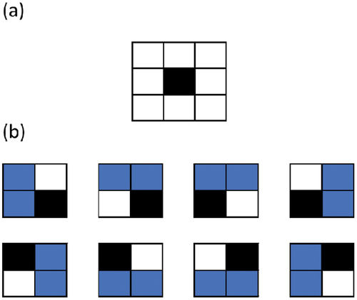
Only the blocks resulting in operationally feasible shapes are considered candidates during the clustering procedure. Thus, a candidate block must be adjacent to at least two blocks that belong to the same cluster, as illustrated by Figure 1. The exception to this constraint is when clusters are composed of just the block reference. In this case, the neighbours in the four main directions (up, down, left, right) are considered.

Figure 1. Illustration of a potential (a) block candidate, in black, where at least one of the options (b) of neighbours belonging to the same (blue) cluster is required for a block to be a candidate.

Each cluster $c_j$ has a set ${\mathcal{P}}_j$ of candidate blocks $x_i\in {\mathcal{P}}_j$ available for merging, and $\mathcal{P}$ is the set containing all candidate blocks. Thus, the block $x_m$ incurring the smallest loss will be selected to merge with the related cluster $c_k$:

(6) $x_m=\underset{x_i\in P_k{P}_k\in P}{\min }Loss\left(c_k\cup x_i\right)$(6)

A priority queue is created to keep the loss values ordered to avoid searching the entire list of possible candidates at every step, facilitating the search. The clustering algorithm generating diglines, illustrated in Figure 2, is defined as follows:

Table

Clustering algorithm
Input
Simulated orebody models ${\mathcal{S}}_{geo}$ Cluster reference $x_j\in B_{fix}$ Initial clusters $c_j\in \mathcal{C}$, associated with $x_j$
Output
Final clusters $c_j\in \mathcal{C}$
Procedure
(1)	Get the initial set of block candidates $x_i\in {\mathcal{P}}_j$
(2)	Get the loss function-based distance $\left(x_i;c_j\right),\hspace{0.17em}\mathrm{\forall }{x}_i\in {\mathcal{P}}_j,$ $\mathrm{\forall }{c}_j\in \mathcal{C}$. Create a sorted queue for all $d\left(x_i;c_j\right)$ values
(3)	While there are blocks to be merged
(3.1)	Merge the block $x_i$ with cluster $c_j$ having the smallest loss value.
(3.2)	Remove $x_i$ from ${\mathcal{P}}_j$ and $\mathcal{P}$ and update the candidates ${\mathcal{P}}_j$ associated with $c_j$.
(3.3)	If $\left|c_j\right|=N_{max}$:
(3.3.1)	Remove $c_j$ from the set of eligible clusters.
(3.4)	Else:
(3.4.1)	Recalculate all loss function-based distances $d\left(x_{i{ }^{\mathrm{\prime }}};c_j\right)$ associated with $c_j$, $\mathrm{\forall }{x}_{i{ }^{\mathrm{\prime }}}\in {\mathcal{P}}_j$
(4)	For $c_j\in \mathcal{C}$:
(4.1)	If $\left|c_j\right|<N_{min}:$
(4.1.1)	Post-process the model to achieve the minimum size requirement.

Figure 2. Illustration of the clustering algorithm at different steps (a)-(d) and destination decisions (e).

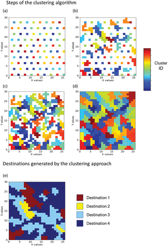
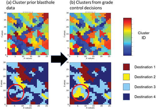
When blasthole data is available, the ensemble Kalman filter method (EnKF) [33,35,63] is applied to update the set of simulated orebody models. This modifies the current knowledge about the spatial distribution of grades over the related area, modifying the destination decisions obtained with the clustering algorithm. These are now the grade control decisions obtained with blasthole data. Note that the number of clusters is constant as the cluster references are fixed, even though the diglines can be rearranged in space. Figure 3 shows an example of incorporating data from the area highlighted by the red circle. This can modify locally the digline definitions.

Figure 3. Local updating of the spatial clusters given the blasthole information incorporated into the orebody model.

2.2. Actor-critic approach to short-term planning considering shovel allocation and grade control decisions

The proposed actor-critic method consists of an RL agent [16] and a simulator of the mining complex operations based on discrete event simulation [37] and system dynamics [38]. The RL agent is responsible for defining shovel allocation and, consequently, extraction sequence while obtaining classification and digline definitions from grade control. The mining complex environment emulates the mining operations, such as loading, transportation and processing, which result from the shovel allocation decisions taken by the RL agent. A reward score associated with the operation’s financial performance is also provided by the simulator of the mining complex, which is used to train the RL agent. The following subsections describe the main aspects of the RL agent applied to the short-term planning of mining complexes, the associated environment and the learning algorithm.

2.2.1. Reinforcement learning agent architecture

The RL agent is responsible for assigning shovels to benches in the mines of a mining complex. During the shovel allocation, operational requirements are of extreme importance. Therefore, the clustering algorithm provides mineable shapes to be used as inputs by the actor-critic method. Then, denote $s{h}_{h,c_j,t}$ as the action associated with shovel $h\in \mathcal{H}$ mining the cluster $c_j$ at time step $t\in \mathbb{T}=\left\{1,2,\dots ,\mathcal{T}\right\}$. The RL agent is composed of an actor that outputs the policy function $\pi \left(s{h}_{h,c_j,t}|Stat{e}_t,\theta \right)$, providing probabilities associated with each action given the state $Stat{e}_t\in \mathbb{S}$ and neural network parameters $\theta$. This policy function is represented in Figure 4.

Figure 4. Architecture of neural network representing the RL agent.

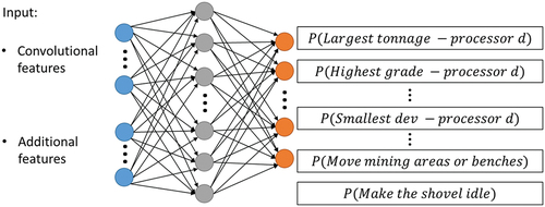
The inputs shown in Figure 4 represent the state $Stat{e}_t$ at time step $t$ observed by the RL agent, which is a numerical description of the mining complex. There are two types of inputs: a convolutional part and some additional features. The convolutional inputs consider the three-dimensional spatial configuration of the orebody model and selected attributes. These features are 0–1 coded values related to the mined and exposed blocks, the trajectory of the shovel in consideration and the current locations of other shovels. For additional features, general aspects regarding the mining complex are included:

• Grade control features: encompass the simulated grade values associated with the available digline clusters. The values are divided by the maximum grade to keep values between 0 and 1. The total tonnage is also a feature standardised between 0 and 1.

• Mining complex features: consider the past performance of the mining complex, such as past daily tonnages extracted per mine, head grades feeding the different processors, and tonnage throughput at the crushers and processors.

• Different shovel features: comprise grades of the mining blocks being extracted by all shovels, except the one requesting a new assignment. It is also inputted the processor destination provided by the digline cluster, using the one-hot-encoding strategy, and how many blocks still need to be extracted by these shovels.

• Equipment features: relate to current equipment capacities.

• Downstream features: contain information about the current performance of the mining complex regarding the quantity being processed, targets, head grades, and grade requirements for deleterious elements.

To fully describe the output space of the RL agent, denote each mine as $m\in \mathcal{M}$, being $\mathcal{M}$ the set containing all mines. m can be subdivided into mining areas and working benches $m_{r,l}$. $r$ denotes the mining areas provided by short-term planning assumptions, and $l$ is used to index the associated benches. The processors considered are defined by $d\in \mathcal{D}$. The output of the neural network, illustrated in Figure 4, is described as the digline presenting the following:

• Largest tonnage feeding the processor $d$ in $m_{r,l}$;

• Largest metal content feeding processor $d$ in $m_{r,l}$;

• Largest metal grade feeding processor $d$ in $m_{r,l}$;

• Smallest deviation associated with element $a\in \mathcal{A}\hspace{0.17em}$feeding processor $d$ in $m_{r,l}$;

• Closest digline cluster in $m_{r,l}$ from the accessing ramp and feeding the processor $d$;

• Smallest tonnage feeding the waste dump $d$ in $m_{r,l}$;

• Smallest metal content feeding the waste dump in $m_{r,l}$;

• Smallest metal grade feeding the waste dump in $m_{r,l}$;

There is also a critic designed to approximate the state value function $v\left(Stat{e}_t,\omega \right)$, given neural network parameters $\omega$, that estimates the expected cumulative reward, as shown in Equation. 7:

(7) $v\left(S_t,\omega \right)\approx E_{\pi }\left[R_t|Stat{e}_t\right]$(7)

The architecture of the critic is almost identical to the actor $\pi \left(s{h}_{h,c_j,t}|Stat{e}_t,\theta \right)$, except by the last layer, where the critic only outputs one value.

Choosing one of the actions mentioned above implies that the shovel is going to be assigned to a specific cluster $c_j$. The same cluster may be associated with more than one action. When a shovel finishes an assignment, it requests a new destination decision to be provided by the RL agent. Moving to distant regions incurs production losses, and the allocation policy must balance the desirability to mine profitable areas and moving costs. Only feasible actions are allowed; thus, the following constraints are respected:

• Each cluster can be mined only once and by one shovel:

  (8) $\sum _{t\in \mathbb{T}}\sum _{h\in \mathscr{H}}s{h}_{h,c_j,t}\le 1,\forall c_j\in \mathcal{C}$(8)

• The cluster must be exposed regarding the vertical predecessors:

  (9) $s{h}_{h,c_j,t}\le \sum t\prime =0t-1\sum _{h\in \mathscr{H}}shh,cj\prime ,t,\forall cj\prime \in VertPred\left(c_j\right);t\in \mathcal{T};h\in \mathscr{H}$(9)

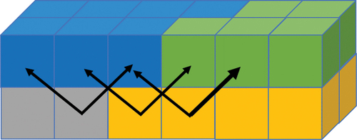
where $VertPred\left(c_j\right)$ is the set of vertical predecessors of the cluster $c_j$, comprising all blocks lying above the related cluster given slope requirements. Figure 5 illustrates these vertical constraints. They are very similar to traditional slope constraints. The only additional aspect is that the cluster configuration can require angles that are smaller than the one required by a single block. All predecessor blocks must be accessible to extract a certain cluster. Since these predecessors may belong to different clusters, all these clusters must be entirely mined to expose the below one. The example in Fig. Figure 55 shows the case where both the green and blue clusters are predecessors of the orange cluster, while the grey one has only the blue cluster as a predecessor.

Figure 5. Illustration of the vertical constraints applied to clusters.

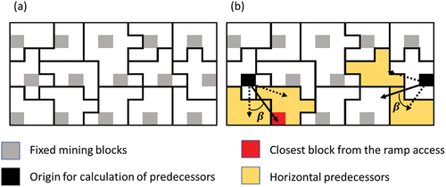
• The cluster must be exposed regarding the horizontal predecessors:

(10) $s{h}_{h,c_j,t}\le \sum _{h\in \mathscr{H}}\sum t\prime =0t-1shh,cj\prime ,t,\forall cj\prime \in HorzPred\left(c_j\right);t\in \mathcal{T};h\in \mathscr{H}$(10)

where $HorzPred\left(c_j\right)$ is the set of horizontal predecessors of $c_j$, based on [61]. The related blocks are obtained based on the direction from the cluster reference towards the ramp access and given a horizontal angle, as shown in Figure 6.

Figure 6. Illustration of clusters’ (a) geometries and (b) set of predecessors obtained from the related cluster reference towards the ramp access.

2.2.2. Simulator of mining complex operations

The learning process associated with the actor-critic method described in the next section requires that the agent observes different states and rewards. Thus, this section briefly describes a simulator of the mining complex operations to forecast the material flow from the mining benches to the related mineral processor. This simulator is modelled based on discrete event simulation [37] and emulates daily operations such as extraction, haulage, and processing activities. Thus, for every simulated day of operation day $p\in \left\{1,\dots ,N_{days}\right\}$, the simulator forecasts the associated material flow given the allocation decisions provided by the RL agent. $N_{days}$ represents the number of days simulated, which is referred as episode herein.

Many mining operations are characterised by uncertainties, summarised here in terms of equipment performance. The set of realisations representing equipment uncertainty is denoted by ${\mathcal{S}}_{equip}$. Thus, the productivity of each shovel $h\in \mathcal{H}$ and crusher $k\in \mathcal{K}$ is denoted by $pro{d}_{h,s_e,p}$ and $pro{d}_{k,s_e,p}$, respectively. The destination decision of the material from the benches is defined by the grade control clustering algorithm, which will also associate an available crusher to the shovel. Then, ${\mathcal{H}}_k$ denotes the set of shovels associated with crusher $k$. Given the configuration of the mining complex, as described in the ‘Case study’ section, each crusher can be associated with processor destinations $d\in \mathcal{D}$. Thus, $\mathcal{K}$ denotes the set of crushers that can send material to destination $d$. The production of each destination is expressed by $pro{d}_{d,s_e,p}$ and its maximum capacity by $ca{p}_d$. Additionally, it is assumed that each processor has a stockpile associated with stabilising production, whose amount of material is defined by $stk{p}_{d,s_e,p}$. Thus, a summary of the simulation associated with these mining operations is described below for every day represented by $p$:

Table

Simulate daily operations algorithm
Input
Current period $p$ Simulated equipment capacities ${\mathcal{S}}_{equip}$ Simulated orebody models ${\mathcal{S}}_{geo}$ Shovel allocation decisions $s{h}_{h,c_j,t}\mathrm{\forall }h\in \mathcal{H}$
Output
Shovel and crusher capacities, $pro{d}_{h,s_e,p}$ $\mathrm{\forall }h\in \mathcal{H}$ and $pro{d}_{k,s_e,p}$ $\mathrm{\forall }k\in \mathcal{K}$ Destination throughput $pro{d}_{d,s_e,p}\mathrm{\forall }d\in \mathcal{D}$ Stockpile material $stk{p}_{d,s_e,p+1}$ And associated material quality at the destinations
Procedure
(1)	Sample equipment scenario $s_e\in {\mathcal{S}}_{equip}$, defining $ca{p}_{h,s_e,p},\hspace{0.17em}\mathrm{\forall }h\in \mathcal{H}$ and $ca{p}_{k,s_e,p},\hspace{0.17em}\mathrm{\forall }k\in \mathcal{K}$.
(2)	If $\left({\sum }_{h\in {\mathcal{H}}_k}pro{d}_{h,s_e,p}\right)\ge pro{d}_{k,s_e,p}$:
(2.1)	$pro{d}_{h,s_e,p}=pro{d}_{h,s_e,p}\cdot \frac{pro{d}_{k,s_e,p}}{{\sum }_{h\in {\mathcal{H}}_k}pro{d}_{h,s_e,p}},\hspace{0.17em}\mathrm{\forall }h\in {\mathcal{H}}_k;k\in \mathcal{K}$
(3)	Else:
(3.1)	$pro{d}_{k,s_e,p}={\sum }_{h\in {\mathcal{H}}_k}pro{d}_{h,s_e,p},\hspace{0.17em}\mathrm{\forall }k\in \mathcal{K}$.
(4)	If $\sum _{k\in {\mathcal{K}}_d}pro{d}_{k,s_e,p}\ge ca{p}_d:$
(4.1)	$pro{d}_{d,s_e,p}=ca{p}_d,\hspace{0.17em}\mathrm{\forall }d\in \mathcal{D}$.
(4.2)	$stk{p}_{d,s_e,p+1}=stk{p}_{k,s_e,p}+\left({\sum }_{k\in {\mathcal{K}}_d}pro{d}_{k,s_e,p}-ca{p}_d\right)$.
(5)	Else:
(5.1)	If $\left({\sum }_{k\in {\mathcal{K}}_d}pro{d}_{k,s_e,p}+stk{p}_{d,s_e,p}\right)\ge ca{p}_d:$
(5.1.1)	$pro{d}_{d,s_e,p}=ca{p}_d,\hspace{0.17em}\mathrm{\forall }d\in \mathcal{D}$.
(5.1.2)	$stk{p}_{d,s_e,p+1}=stk{p}_{d,s_e,p}-\left(ca{p}_d-{\sum }_{k\in {\mathcal{K}}_d}pro{d}_{k,s_e,p}\right)$.
(5.2)	Else:
(5.2.1)	$pro{d}_{d,s_e,p}=stk{p}_{d,s_e,p}+{\sum }_{k\in {\mathcal{K}}_d}pro{d}_{k,s_e,p},\mathrm{\forall }d\in \mathcal{D}$.
(5.2.2)	$stk{p}_{d,s_e,p+1}=0$.

Since the position of the shovel equipment is known and it is linked to mining blocks $x_i$, the characteristics and quantities of the material extracted by shovel $h$ can be calculated.

As mentioned earlier, it is considered that the mining complex incorporates blasthole information. These data are received at fixed time steps, and the simulated orebody model is updated based on the EnKF approach. This updating step is embedded in the mining complex simulator such that it also influences the mining complex state.

2.2.3. Actor-critic reinforcement learning approach

During an episode representing the simulation of the mining operations, a shovel can request allocation decisions, where each one defines a time step $t\in \mathbb{T}=\left\{1,2,\dots ,\mathcal{T}\right\}$, given the observation of the state of the mining complex $Stat{e}_t\in \mathbb{S}$ described in the ‘Reinforcement learning agent architecture’ section. After each allocation decision, a reward score is calculated and used in the learning procedure so that the agent can differentiate between good and bad actions. This reward $r_t$ is defined as the temporal difference between two consecutive utility function values:

(11) $r_t=u\left({\tau }_{t+1}\right)-u\left({\tau }_t\right)$(11)

where ${\tau }_t$ is the trajectory since the initial time step $t=0$ and the related changes in the mining complex space:

(12) ${\tau }_t=\left(\left(Stat{e}_0,s{h}_{h,c_j,0},r_1\right),\left(Stat{e}_1,s{h}_{h,c_j,1},r_2\right),\dots ,\left(Stat{e}_{t-1},s{h}_{h,c_j,t-1},r_t\right)\right)$(12)

The utility function is then calculated as follows:

(13) $u\left({\tau }_t\right)=\sum t\prime =1t\sum d\in D\frac{1}{\left|S\right|}\sum s\in S_{geo}\sum a\in Arevd,a,s,t\prime -devd,a,s,t\prime -proc\_costd,t\prime -min\_costt\prime -pen\_shov\_movt\prime$(13)

where $re{v}_{d,a,s,t}$ is the revenue obtained by selling the product related to geological attribute $a\in \mathcal{A}$ under the stochastic scenario $s\in {\mathcal{S}}_{geo}$ processed by destination $d\in \mathcal{D}$ at time $t$. $de{v}_{d,a,s,t}$ is the penalty applied for deviating from the production targets associated with element $a$. This is calculated by the absolute difference between the daily target and the related attribute calculated for the blend material at processor $d$. This absolute value is multiplied by a user-defined positive cost factor to prioritise different targets and to compare attributes with different units. $proc\mathrm{\_}cos{t}_{d,t}$ is the processing cost in destination $d$. $min\mathrm{\_}cos{t}_t$ is the mining cost that considers the loading and hauling activities. Finally, $pen\mathrm{\_}shov\mathrm{\_}mo{v}_t$ is the penalty applied due to lost tonnes from relocating shovels to distant locations. This penalty is calculated by multiplying the shovel relocation time by its productivity and by a user-defined cost factor to compare this value with the other financial components of Equation. 13. Then, the cumulative reward $R_t$ is defined as:

(14) $R_t=\sum t\prime =\text{t}T\gamma t\prime -trt\prime$(14)

where $\gamma$ is the discounting factor that gives smaller weights to rewards in the distant future. The RL approach focuses on maximising the expected cumulative reward $R_t$:

(15) $\begin{array}{c}\underset{s{h}_{h,c_j,t}}{max}{E}_{\pi }\left[R_t|Stat{e}_t\right]\end{array}$(15)

The outcome of each decision made by the RL agent, meaning the related material flow from the benches to the processors, is forecasted according to the ‘Simulator of mining complex operations’ section, respecting the related operational constraints. Given the reward received from this forecast, the critic guides the actor to make improved decisions through the calculation of the advantage function:

(16) $\mathcal{A}\left(Stat{e}_t,Stat{e}_{t+1},\omega \right)=r_t+\gamma \cdot v\left(Stat{e}_{t+1},\omega \right)-v\left(Stat{e}_t,\omega \right)$(16)

which is used to update the neural network weights from both actor and critic through gradient descent and backpropagation:

(17) ${\theta }_{k+1}\leftarrow {\theta }_k+{\alpha }_{\theta }\mathcal{A}\left(Stat{e}_t,Stat{e}_{t+1},{\omega }_k\right)\nabla \ln \left(\pi \left(s{h}_{c_j,t,h}|Stat{e}_t,{\theta }_k\right)\right)$(17)

(18) ${\omega }_{k+1}\leftarrow {\omega }_k+{\alpha }_{\omega }\mathcal{A}\left(Stat{e}_t,Stat{e}_{t+1},{\omega }_k\right)\nabla v\left(Stat{e}_t,{\omega }_k\right)$(18)

where ${\alpha }_{\theta }$ and ${\alpha }_{\omega }$ are the learning rate of the actor and critic, respectively. Future work can investigate different architectures and techniques to enhance the convergence and generalisation of the proposed approach. The algorithm is summarised as follows:

Table

Actor critic algorithm for short-term mine planning
Input
Simulated orebody models ${\mathcal{S}}_{geo}$ at point and block support Simulated blasthole data at point support ${\mathcal{S}}_{gc}$ Initial shovel allocations $s{h}_{h,c_j,-1}\mathrm{\forall }h\in \mathcal{H}$ Number of training iterations $N_{training}$
Output
Trained shovel allocation policy $\pi \left(s{h}_{h,c_j,t}|Stat{e}_t,{\theta }_t\right)$
Procedure
(1)	Run the Clustering algorithm presented in the “Clustering algorithm based on the minimum loss function” section.
(2)	Randomly initialise the parameters $\theta$ and $\omega$ of the RL agent.
(3)	Halve the set ${\mathcal{S}}_{geo}$ into (${\mathcal{S}}_{geo}^{train},{\mathcal{S}}_{geo}^{test}$) and ${\mathcal{S}}_{gc}$ into (${\mathcal{S}}_{gc}^{train},{\mathcal{S}}_{gc}^{test}$).
(4)	For $0\le ep\le$ $N_{training}$ do:
(4.1)	Sample one $s_{gc}\in {\mathcal{S}}_{gc}^{train}$
(4.2)	For $0\le t\le N_{days}$ do:
(4.2.1)	Run the Simulate daily operations, presented in the Simulator of mining complex operations section
(4.2.2)	If a shovel $h$ requests a new allocation:
(4.2.2.1)	Get $s{h}_{h,c_j,t}$from $\pi \left(s{h}_{h,c_j,t}|Stat{e}_t,{\theta }_t\right)$.
(4.2.2.2)	Store $v\left(Stat{e}_t,{\omega }_t\right)$ and $v\left(Stat{e}_{t+1},{\omega }_t\right)$, the obtained reward $r_t$ (Equations. 11 and 13) and the log probability $log\left(\pi \left(s{h}_{h,c_j,t}|Stat{e}_t,{\theta }_t\right)\right)$.
(4.2.2.3)	If a subset of $s_{gc}$ is assumed available:
(4.2.2.3.1)	Use EnKF to locally update${\mathcal{S}}_{geo}^{train}$ at the point-support
(4.2.2.3.2)	Upscale the updated orebody simulations to block-support
(4.2.2.3.3)	Run the Clustering algorithm locally on the updated blocks
(4.3)	Get the cumulative reward $R_t$, according to Eq. 14
(4.4)	Update the neural network parameters according to Equations 16, 17 and 18

Additionally, Figure 7 presents a schematic diagram illustrating how the clustering and the reinforcement learning applied to short-term planning methods are connected. Each method could be applied sequentially. However, the framework presented proposes to update the clusters given incoming grade-control data within the short-term planning model. This approach aims to capitalise on new information that can change short-term decision making and presents an adaptive framework that can propose the extraction sequence, destinations, and shovel allocation decisions in response.

Figure 7. Workflow of the proposed method.

3. Case study

3.1. Overview of the industrial mining complex

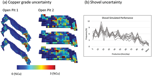
The proposed actor-critic method is applied to an operating copper mining complex whose configuration is presented in Figure 8. The materials are extracted from two open-pit mines and can feed different mills, leach pads or sent to the waste dump. A crusher circuit is necessary to deliver the proper comminution requirements size for selected processing routes. The main goal of the mining operation is to maximise profit by improving copper production. The uncertainty and variability associated with this geological attribute are modelled by the sequential direct block-support Gaussian simulation method [70,71]. Thus, 10 stochastic simulations characterise the spatial distribution of the copper grades in each mine, as illustrated in Figure 9a. The whole operation also considers 17 shovels with different capacities and performances. Fourteen shovels operate in Open Pit 1, and the remaining three in Open Pit 2. The associated uncertainty of these attributes is represented by 50 simulations obtained from historical data [61], illustrated in Figure 9b. Crusher capacities are also sampled from historical data, describing the uncertainty related to this equipment.

Figure 8. Diagram of the copper mining complex.

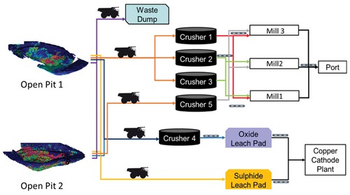
Figure 9. Different sources of uncertainty characterising the copper mining complex.

3.2. Defining grade control diglines

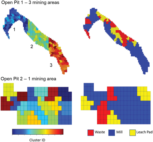
Open Pit 1 is organised in three mining areas, while Open Pit 2 has only one, as illustrated in Figure 10. Also, the clustering approach is applied individually to each mining area, where operational equipment requirements are respected.

Figure 10. Grade control algorithm applied to initial simulations associated with open pit 1 and open pit 2.

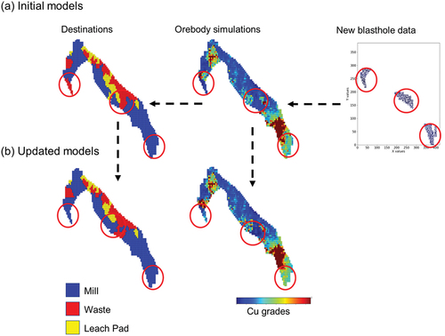
Blasthole data arrives at the end of every week. These data are mapped into the orebody model and used to update the uncertainty associated with the geological attributes using EnKF, as illustrated in Figure 11a. Next, this updated orebody model is inputted into the clustering algorithm, which, in turn, updates locally the digline definitions and destination decisions, as shown in Figure 11b. This process is embedded in the simulator of the mining complex operations, discussed in the ‘Simulator of mining complex operations’ section.

Figure 11. Illustration of the updating approach, where the blasthole data are mapped in the orebody model (a), and then, the orebody models and the diglines are updated (b).

3.3. Adaptive scheduling decisions and production forecast

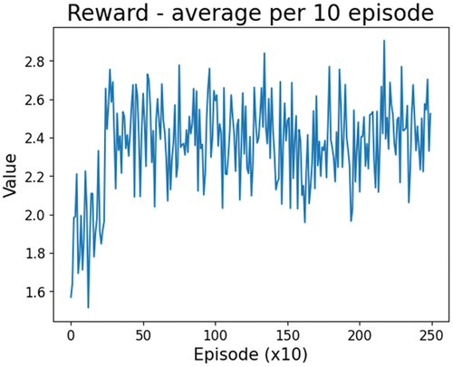
In the actor-critic framework proposed, each episode emulates 30 days of operations using the simulator of the mining complex. These episodes are repeated 2500 times and are used to train the RL agent. This required approximately 24 hours on an Intel® Xeon® CPU E5–2650 v4 with 2.20 GHz, running Oracle Linux Server 7.9 and with an NVIDIA Tesla P100 PCIe 12GB GPU. The RL agent’s complete architecture is presented in the Appendix for additional information. Figure 12 shows the learning curve displaying the cumulative reward per episode averaged every 10 episodes. As a general trend, the curve shows a quick increase for the first 500 iterations and reaches a plateau afterwards. Some oscillation occurs, which is typical of actor-critic approaches, and probably enhanced by the different sources of stochasticity of the mining complex and also due to the large state space the RL agent perceives. Herein, the choice for training for 2500 episodes is due to the stabilisation of the cumulative reward value after a quick drop around 1500 episodes. Future work should focus on improving the architecture of the RL agent and related parameters to improve this learning behaviour.

Figure 12. Cumulative reward averaged at every 10 episodes.

After the training, one additional episode of the mining complex model is triggered; the results regarding the extraction sequence and shovel allocation strategy are shown below. The results obtained with the proposed actor-critic approach are referred to as the RL case. For comparison, a sequential optimisation approach is used as a baseline, which is composed of three parts. First, the extraction sequence is provided by the previous advancement in the field [39]. This previously optimised extraction sequence generates results showing financial improvements over a conventional short-term plan applied by the mine. This original approach does not include grade control, nor it is capable of directly allocating multiple shovels. Then, the proposed grade-control cluster algorithm is applied and the diglines are defined. Next, the forecast of the baseline case is assessed by the simulator of mining complex operations presented in the ‘Simulator of mining complex operations’ section. Then, every time a shovel requests a new assignment, the baseline case applies a heuristic approach that minimises shovel movement between scheduled diglines.

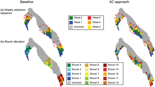
Figure 13 compares the extraction sequence obtained by the baseline and the RL approach. Initially, there are four, five and five shovels in areas 1, 2 and 3, respectively. The baseline schedule presents a more practical allocation strategy because the shovels are assigned to the closest location after finishing their tasks. Conversely, the RL case allows shovels to move between areas according to the current mining complex requirements, which results in very different extraction sequences. Some differences are related to the period in which the material is extracted, exemplified in mining area 1. But the more important ones are due to the preference for extracting material from different locations, as observed in mining areas 2 and 3. The red circles in Figure 13 highlight these major differences. Additionally, the RL and baseline cases extract a similar amount of material from mining areas 1 and 3, but the volume extracted in mining area 2 is significantly different. The RL approach assigns more shovels to increase production in this region. This illustrates the model’s flexibility, allowing the shovels to move according to different needs.

Figure 13. Weekly extraction sequence (a) and shovel allocation decisions (b) for open pit 1 obtained by the baseline and RL approaches. The red circles highlight the differences in both schedules.

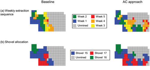
Figure 14 presents similar results for Open Pit 2. As this pit has only one mining area, the shovel allocation from both strategies results in similar and practical schedules. Even in this more constrained configuration, there are large differences in the schedules obtained, confirming the proposed method’s ability to adapt decisions when facing uncertainty and incoming information.

Figure 14. Weekly extraction sequence (a) and shovel allocation decisions (b) for open pit 2 obtained by the baseline and RL approaches.

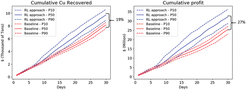
To assess the production forecast at different destinations, 10 episodes of the simulator of the mining complex operations are repeated. The results are presented below in terms of P10, P50 and P90, representing the 10^th, 50^th and 90^th percentile. Figure 15 shows the ore throughput at Mill 1 and Mill 3 and the amount of material sent to the waste dump obtained with the baseline and RL approaches. Concerning mill throughout, both approaches can process a similar ore quantity, where the capacity is nearly always reached. But more importantly, the copper profile shows interesting differences, as shown in Figure 16. The RL case forecasts substantially more metal being recovered over the 30 days of simulated operation. This suggests that the RL agent learns to adapt the production plan given the change in destination decisions provided by the updates in the digline definitions. Regarding the waste dump, the baseline approach extracts more waste than the RL case. This difference can be explained by the reward function maximising the overall profit; thus, recovering more metal is more important than satisfying tonnage targets. The result is a policy more concerned with the quality of material feeding the processors. Nonetheless, the RL approach still mines a good portion of waste, which is important to expose ore in future periods. Considering all the above aspects, the RL approach generates 27% more cash flow than the baseline, demonstrating a great improvement for short-term planning, as illustrated in Figure 16.

Figure 15. Forecast of the ore throughput for Mill 1 and Mill 3 and tonnages at the waste dump obtained using the baseline and RL approaches.

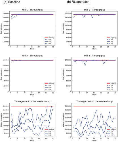
Figure 16. Cumulative copper profile recovered by all processors and the associated cumulative profit.

4. Conclusions

This paper presents a new actor-critic RL approach providing adaptive short-term planning decisions by defining shovel allocation while accounting for digline definitions obtained from a spatial clustering algorithm. The clustering algorithm presented determines groups of spatially connected mining blocks with similar processing performances. The algorithm uses loss functions as the distance metric to be minimised. Once blasthole data arrives, the algorithm updates decisions defining grade control diglines. This considers the impact of simultaneously processing blended materials. The generated diglines are assumed to provide feasible shovel allocations. Concerning the proposed actor-critic reinforcement learning framework, an RL agent is represented by a neural network architecture that provides allocation decisions given the current requirements and configuration of the mining complex. Each allocation decision associates a shovel to a certain digline location. Also, a simulator of the mining complex operations is proposed, as required by the RL approach. Given the shovel allocation decisions, it forecasts the material flow from mining benches to processors. The uncertainties associated with metal grades and equipment performance are incorporated. Additionally, the orebody model updating and clustering approaches are embedded into the simulator of the mining complex operations.

A case study at a copper mining complex, composed of two open pit mines, four mining areas, three processing mills, leaching pads, a waste dump, crushers and seventeen shovels, is investigated. The results of the proposed method are compared with a baseline approach, where the schedule was obtained from a previous short-term planning approach. The production is forecasted by the simulator of the mining complex operations presented, and the shovel allocation is defined by a heuristic approach minimising shovel movement. The results show that the proposed approach can adapt to different mining complex configurations and incoming blasthole data, illustrated by the differences in extraction sequences. However, the most important differences are observed when analysing the copper profile, where the RL approach produces substantially more copper. This provides cash flow earlier to the operation, increasing it by 27% at the end of 30 days of the simulated operations.

Future work should focus on studying different output and input space architectures of the RL agent. The idea is to decrease the model size and speed up the learning process. Another aspect to be considered is a major integration of reinforcement learning approaches and mathematical programming models. For example, including RL adaptive approaches in the long-term simultaneous stochastic optimisation of mining complexes. This would allow more operational aspects to be incorporated into the long-term simultaneous stochastic production planning framework.

Acknowledgments

The work in this article was supported by the National Sciences and Engineering Research Council of Canada (NSERC) under CDR Grant 500414-16 and NSERC Discovery Grant 239019; the mining industry consortium members of McGill’s COSMO Stochastic Mine Planning Laboratory (AngloGold Ashanti, AngloAmerican, BHP, De Beers, IAMGOLD, Kinross, Newmont, and Vale); and the Canada Research Chairs Program.

Disclosure statement

No potential conflict of interest was reported by the authors.

Appendix

Appendix

Figure A1 presents the complete neural network architecture of the RL agent in the actor-critic, which is described in the ‘Reinforcement learning agent architecture’ section and is applied in the ‘Case study’ section. Since the case study considers two open pits, the neural network presented considers three types of inputs, convolutional features of Open Pit 1, convolutional features of Open Pit 2 and additional features. The input sizes of the convolutional layers are related to the size of the mining benches considered. For example, Open Pit 1 has a three-dimensional structure of 88 × 77x2 blocks. There are two benches and a rectangular shape of 88 × 77 blocks on each level. The blocks already mined out previously were padded with zeros concerning all attributes. The output layer is associated with the possible shovel allocation decisions described previously.

Figure A1. Neural network architecture related to the RL agent.

No pre-trained layers were used during the training process. Still, the field of transfer learning should be investigated in future studies as this has the potential to speed up the training part and improve the generalisation capacity of the RL agent. The kernel size was selected considering the number of mining benches and a small number of blocks of x and y directions that would approximate the number of blocks present in a cluster. Dropout layers were selected through trial and error. Note that future work can focus on improving the architecture of the RL agent using a grid search approach, as these parameters can impact both solution and convergence time.

References

- K. Fytas and P.N. Calder, A computerized model of open pit short and long range production scheduling, 19th Application of Computers and Operations Research In the Mineral Industry, State College, USA, 1986, pp. 109–119.
- M. Blom, A.R. Pearce, and P.J. Stuckey, Short-term planning for open pit mines: A review, Int. J. Mining, Reclam. Environ 33 (5) (2019), pp. 318–339. doi:10.1080/17480930.2018.1448248.
- W.A. Hustrulid, M. Kuchta, and R.K. Martin, Open Pit Mine Planning & Design, 3rd ed.CRC ed., Press, London, UK, 2013.
- G. L’Heureux, M. Gamache, and F. Soumis, Mixed integer programming model for short term planning in open-pit mines, Trans. Institutions Min. Metall. Sect. A Min. Technol 122 (2) (2013), pp. 101–109. doi:10.1179/1743286313Y.0000000037.
- A.M. Afrapoli and H. Askari-Nasab, Mining fleet management systems: A review of models and algorithms, Int. J. Mining, Reclam. Environ 33 (1) (2019), pp. 42–60. doi:10.1080/17480930.2017.1336607.
- N. Schofield and P. Rolley, Optimisation of ore selection in mining: Method and case studies, in Proceedings of the Mining Geology Conference, AusIMM, Launceston, TAS, Australia, 1997, pp. 93–97.
- M.E. Rossi and C.V. Deutsch, Mineral Resource Estimation, Springer Netherlands, Dordrecht, 2014. doi:10.1007/978-1-4020-5717-5.
- R. Dimitrakopoulos and M. Godoy, Grade control based on economic ore/waste classification functions and stochastic simulations: Examples, comparisons and applications, Min. Technol. 123 (2014), pp. 90–106. doi:10.1179/1743286314Y.0000000062.
- R. Dimitrakopoulos and A. Lamghari, Simultaneous stochastic optimization of mining complexes - mineral value chains: An overview of concepts, examples and comparisons, Int. J. Mining, Reclam. Environ 36 (6) (2022), pp. 443–460. doi:10.1080/17480930.2022.2065730.
- L. Montiel and R. Dimitrakopoulos, Simultaneous stochastic optimization of production scheduling at Twin Creeks mining complex, Nevada, Min. Eng. 70 (2018), pp. 48–56. doi:10.19150/me.8645.
- R. Goodfellow and R. Dimitrakopoulos, Simultaneous stochastic optimization of mining complexes and mineral value chains, Math Geosci 49 (3) (2017), pp. 341–360. doi:10.1007/s11004-017-9680-3.
- M.F. Del Castillo and R. Dimitrakopoulos, Dynamically optimizing the strategic plan of mining complexes under supply uncertainty, Resour. Policy 60 (2019), pp. 83–93. 10.1016/j.resourpol.2018.11.019.
- A. Kumar and R. Dimitrakopoulos, Application of simultaneous stochastic optimization with geometallurgical decisions at a copper–gold mining complex, Min. Technol. 128 (2019), pp. 88–105. doi:10.1080/25726668.2019.1575053.
- C. Both and R. Dimitrakopoulos, Utilisation of geometallurgical predictions of processing plant reagents and consumables for production scheduling under uncertainty, Int. J. Mining, Reclam. Environ 37 (1) (2023), pp. 21–42. doi:10.1080/17480930.2022.2139350.
- R. Goodfellow and R. Dimitrakopoulos, Global optimization of open pit mining complexes with uncertainty, Appl. Soft Comput. 40 (2016), pp. 292–304. doi:10.1016/j.asoc.2015.11.038.
- R.S. Sutton and A.G. Barto, Reinforcement Learning : An Introduction, 2nd ed.MIT ed., Press, Cambridge, 2018.
- D. Silver, A. Huang, C.J. Maddison, A. Guez, L. Sifre, G. Van Den Driessche, J. Schrittwieser, I. Antonoglou, V. Panneershelvam, M. Lanctot, S. Dieleman, D. Grewe, J. Nham, N. Kalchbrenner, I. Sutskever, T. Lillicrap, M. Leach, K. Kavukcuoglu, T. Graepel, and D. Hassabis, Mastering the game of go with deep neural networks and tree search, Nature 529 (7587) (2016), pp. 484–489. doi:10.1038/nature16961.
- D. Silver, T. Hubert, J. Schrittwieser, I. Antonoglou, M. Lai, A. Guez, M. Lanctot, L. Sifre, D. Kumaran, T. Graepel, T. Lillicrap, K. Simonyan, and D. Hassabis, A general reinforcement learning algorithm that masters chess, shogi, and go through self-play, Science 362 (6419) (2018), pp. 1140–1144. doi:10.1126/science.aar6404.
- O. Vinyals, I. Babuschkin, W.M. Czarnecki, M. Mathieu, A. Dudzik, J. Chung, D.H. Choi, R. Powell, T. Ewalds, P. Georgiev, J. Oh, D. Horgan, M. Kroiss, I. Danihelka, A. Huang, L. Sifre, T. Cai, J.P. Agapiou, M. Jaderberg, A.S. Vezhnevets, R. Leblond, T. Pohlen, V. Dalibard, D. Budden, Y. Sulsky, J. Molloy, T.L. Paine, C. Gulcehre, Z. Wang, T. Pfaff, Y. Wu, R. Ring, D. Yogatama, D. Wünsch, K. McKinney, O. Smith, T. Schaul, T. Lillicrap, K. Kavukcuoglu, D. Hassabis, C. Apps, and D. Silver, Grandmaster level in StarCraft II using multi-agent reinforcement learning, Nature 575 (7782) (2019), pp. 350–354. doi:10.1038/s41586-019-1724-z.
- M. Hessel, J. Modayil, H. Van Hasselt, T. Schaul, G. Ostrovski, W. Dabney, D. Horgan, B. Piot, M. Azar, and D. Silver, Rainbow: Combining improvements in deep reinforcement learning, 32nd AAAI Conference on Artificial Intelligence, New Orleans, 2018, pp. 3215–3222. doi:10.1609/aaai.v32i1.11796.
- V. Mnih, K. Kavukcuoglu, D. Silver, A.A. Rusu, J. Veness, M.G. Bellemare, A. Graves, M. Riedmiller, A.K. Fidjeland, G. Ostrovski, S. Petersen, C. Beattie, A. Sadik, I. Antonoglou, H. King, D. Kumaran, D. Wierstra, S. Legg, and D. Hassabis, Human-level control through deep reinforcement learning, Nature 518 (7540) (2015), pp. 529–533. doi:10.1038/nature14236.
- C. Paduraru and R. Dimitrakopoulos, Adaptive policies for short-term material flow optimization in a mining complex, Min. Technol. 9009 (1) (2017), pp. 56–63. doi:10.1080/14749009.2017.1341142.
- C. Paduraru and R. Dimitrakopoulos, Responding to new information in a mining complex: Fast mechanisms using machine learning, Min. Technol. 128 (2019), pp. 129–142. doi:10.1080/25726668.2019.1577596.
- A. Kumar, R. Dimitrakopoulos, and M. Maulen, Adaptive self-learning mechanisms for updating short-term production decisions in an industrial mining complex, J Intell Manuf 31 (7) (2020), pp. 1795–1811. doi:10.1007/s10845-020-01562-5.
- A. Kumar and R. Dimitrakopoulos, Updating geostatistically simulated models of mineral deposits in real-time with incoming new information using actor-critic reinforcement learning, Comput Geosci 158 (2022), pp. 104962. doi:10.1016/j.cageo.2021.104962.
- J.P. De Carvalho and R. Dimitrakopoulos, Integrating production planning with truck-dispatching decisions through reinforcement learning while managing uncertainty, Minerals 11 (6) (2021), pp. 587. doi:10.3390/min11060587.
- J.P. De Carvalho and R. Dimitrakopoulos, Integrating short-term stochastic production planning updating with mining fleet management in industrial mining complexes: An actor-critic reinforcement learning approach, Appl. Intell. (2023). doi:10.1007/s10489-023-04774-3.
- S. Iyakwari, H.J. Glass, and S.E. Obrike, Discerning mineral association in the near infrared region for ore sorting, Int. J. Miner. Process. 166 (2017), pp. 24–28. doi:10.1016/j.minpro.2017.06.008.
- M. Dalm, M.W.N. Buxton, and F.J.A. van Ruitenbeek, Discriminating ore and waste in a porphyry copper deposit using short-wavelength infrared (SWIR) hyperspectral imagery, Miner. Eng. 105 (2017), pp. 10–18. 10.1016/j.mineng.2016.12.013.
- M. Dalm, M.W.N. Buxton, and F.J.A. van Ruitenbeek, Ore–waste discrimination in epithermal deposits using near-infrared to short-wavelength infrared (NIR-SWIR) hyperspectral imagery, Math Geosci 51 (7) (2019), pp. 849–875. doi:10.1007/s11004-018-9758-6.
- H. Knapp, K. Neubert, C. Schropp, and H. Wotruba, Viable applications of sensor-based sorting for the processing of mineral Resources, ChemBioeng Rev 1 (3) (2014), pp. 86–95. doi:10.1002/cben.201400011.
- M. Kern, L. Tusa, T. Leißner, K.G. van den Boogaart, and J. Gutzmer, Optimal sensor selection for sensor-based sorting based on automated mineralogy data, J. Clean. Prod. 234 (2019), pp. 1144–1152. doi:10.1016/j.jclepro.2019.06.259.
- J. Benndorf, Closed Loop Management in Mineral Resource Extraction, Springer International Publishing, Cham, 2020.
- T. Wambeke, D. Elder, A. Miller, J. Benndorf, and R. Peattie, Real-time reconciliation of a geometallurgical model based on ball mill performance measurements–a pilot study at the Tropicana gold mine, Min. Technol. Trans. Inst. Min. Metall 127 (3) (2018), pp. 115–130. doi:10.1080/25726668.2018.1436957.
- T. Wambeke and J. Benndorf, A simulation-based geostatistical approach to real-time reconciliation of the grade control model, Math Geosci 49 (1) (2017), pp. 1–37. doi:10.1007/s11004-016-9658-6.
- Á. Prior, R. Tolosana-Delgado, K.G. van den Boogaart, and J. Benndorf, Resource model updating for compositional geometallurgical variables, Math Geosci 53 (5) (2021), pp. 945–968. doi:10.1007/s11004-020-09874-1.
- J. Sturgul, Discrete Simulation and Animation for Mining Engineers, CRC Press, Boca Raton, USA, 2015.
- J.D. Sterman, Business Dynamics - Systems Thinking for a Complex World, Irwin/McGraw-Hill, Boston, USA, 2000.
- A. Kumar and R. Dimitrakopoulos, Production scheduling in industrial mining complexes with incoming new information using tree search and deep reinforcement learning, Appl. Soft Comput. 110 (2021), pp. 107644. doi:10.1016/j.asoc.2021.107644.
- A.G. Journel, Fundamentals of Geostatistics in Five Lessons, Stanford Center for Reservoir Forecasting, Stanford University, 1988. 10.1029/SC008
- R.M. Srivastava, D.R. Hartzell, and B.M. Davis, Enhanced metal recovery through improved grade control, 23rd Application of Computers and Operations Research in the Mineral Industry, Tucson, USA, 1992, pp. 243–249.
- A.G. Journel and P.C. Kyriakidis, Evaluation of Mineral Reserves: A Simulation Approach, Oxford University Press, New York, 2004.
- G. Verly, Grade control classification of ore and waste: A critical review of estimation and simulation based procedures, Math Geol 37 (5) (2005), pp. 451–475. doi:10.1007/s11004-005-6660-9.
- Y.A. Sari and M. Kumral, Dig-limits optimization through mixed-integer linear programming in open-pit mines, J Oper Res Soc 69 (2018), pp. 171–182. doi:10.1057/s41274-017-0201-z.
- K.P. Norrena, C.T. Neufeld, and C.V. Deutsch, An update on automatic dig limit determination, Cent. Comput. Geostatistics Annu. Rep 4 (2002), pp. 1–17.
- E. Isaaks, I. Treloar, and T. Elenbaas, Optimum dig lines for open pit grade control, Proceedings of 9th International Mining Geology Conference, Adelaide, Australia, 2014, pp. 425–432.
- Y.V. Vasylchuk and C.V. Deutsch, Optimization of surface mining dig limits with a practical heuristic algorithm, Mining. Metall. Explor 36 (4) (2019), pp. 773–784. doi:10.1007/s42461-019-0072-8.
- Y. Dagasan, P. Renard, J. Straubhaar, O. Erten, and E. Topal, Pilot point optimization of mining boundaries for lateritic metal deposits: Finding the trade-off between dilution and ore loss, Nat. Resour. Res. 28 (1) (2019), pp. 153–171. doi:10.1007/s11053-018-9380-9.
- A.J. Richmond and J.E. Beasley, Financially efficient dig-line delineation incorporating equipment constraints and grade uncertainty, Int. J. Surf. Mining, Reclam. Environ. 18 (2) (2004), pp. 99–121. doi:10.1080/13895260412331295376.
- M.J.F. Souza, I.M. Coelho, S. Ribas, H.G. Santos, and L.H.C. Merschmann, A hybrid heuristic algorithm for the open-pit-mining operational planning problem, Eur. J. Oper. Res. 207 (2010), pp. 1041–1051. doi:10.1016/j.ejor.2010.05.031.
- J. Elbrond and F. Soumis, Towards integrated production planning and truck dispatching in open pit mines, Int. J. Surf. Mining, Reclam. Environ. 1 (1) (1987), pp. 1–6. doi:10.1080/09208118708944095.
- J.W. White and J.P. Olson, Computer-based dispatching in mines with concurrent operating objectives, Min. Eng. 38 (1986), pp. 1045–1054.
- A.M. Afrapoli, S.P. Upadhyay, and H. Askari-Nasab, A fuzzy logic approach towards truck dispatching problem in surface mines, Int. J. Mech. Prod. Eng 6 (2018), pp. 79–84.
- M. Mohtasham, H. Mirzaei-Nasirabad, and B. Alizadeh, Optimization of truck-shovel allocation in open-pit mines under uncertainty: A chance-constrained goal programming approach, Min. Technol. (2) (2021), pp. 81–100. doi:10.1080/25726668.2021.1916170.
- P.A. Dowd, Risk assessment in reserve estimation and open-pit planning, Trans. Inst. Min. Metall 103 (1994), pp. 148–154. 10.1016/0148-9062(95)97056-O.
- P.J. Ravenscroft, Risk analysis for mine scheduling by conditional simulation, Trans. Inst. Min. Metall. Sect. A. Min. Ind. 101 (1993), pp. 104–108. 10.1016/0148-9062(93)90969-K.
- R. Dimitrakopoulos, Stochastic optimization for strategic mine planning: A decade of developments, J. Min. Sci. 47 (2) (2011), pp. 138–150. doi:10.1134/S1062739147020018.
- R. Dimitrakopoulos, C.T. Farrelly, and M. Godoy, Moving forward from traditional optimization: Grade uncertainty and risk effects in open-pit design, Min. Technol. 111 (2002), pp. 82–88. doi:10.1179/mnt.2002.111.1.82.
- S.P. Upadhyay and H. Askari-Nasab, Dynamic shovel allocation approach to short-term production planning in open-pit mines, Int. J. Mining, Reclam. Environ 33 (1) (2019), pp. 1–20. doi:10.1080/17480930.2017.1315524.
- M.E.V. Matamoros and R. Dimitrakopoulos, Stochastic short-term mine production schedule accounting for fleet allocation, operational considerations and blending restrictions, Eur. J. Oper. Res. 255 (3) (2016), pp. 911–921. doi:10.1016/j.ejor.2016.05.050.
- M. Quigley and R. Dimitrakopoulos, Incorporating geological and equipment performance uncertainty while optimising short-term mine production schedules, Int. J. Mining, Reclam. Environ 34 (5) (2020), pp. 362–383. doi:10.1080/17480930.2019.1658923.
- C. Both and R. Dimitrakopoulos, Joint stochastic short-term production scheduling and fleet management optimization for mining complexes, Optim. Eng. 21 (4) (2020), pp. 1717–1743. doi:10.1007/s11081-020-09495-x.
- G. Evensen, Data Assimilation: The Ensemble Kalman Filter 2nd, Springer, Berlin, Heidelberg, 2009. doi:10.1007/978-3-642-03711-5.
- P. Goovaerts, Geostatistics for Natural Resources Evaluation, Oxford University Press, New York, 1997.
- N. Remy, A. Boucher, and J. Wu, Applied Geostatistics with SGeMs, Cambridge University Press, Cambridge, 2009.
- G. Mariethoz and J. Caers, Multiple-Point Geostatistics: Stochastic Modeling with Training Images, Wiley, Hoboken, 2014.
- T. Hastie, R. Tibshirani, and J.H. Friedman, The Elements of Statistical Learning: Data Mining, Inference, and Prediction 2nd, Springer, New York, 2009. doi:10.1007/978-0-387-84858-7.
- L. Montiel and R. Dimitrakopoulos, A heuristic approach for the stochastic optimization of mine production schedules, J. Heuristics 23 (5) (2017), pp. 397–415. doi:10.1007/s10732-017-9349-6.
- F. Albor and R. Dimitrakopoulos, Stochastic mine design optimisation based on simulated annealing: Pit limits, production schedules, multiple orebody scenarios and sensitivity analysis, Min. Technol. IMM Trans. Sect. A 118 (2) (2009), pp. 79–90. doi:10.1179/037178409X12541250836860.
- M. Godoy, The effective management of geological risk in long-term production scheduling of open pit mines, Ph.D. Thesis, University of Queensland, Brisbane, Qld, Australia, 2003.
- A. Boucher and R. Dimitrakopoulos, Block simulation of multiple correlated variables, Math Geosci 41 (2) (2009), pp. 215–237. doi:10.1007/s11004-008-9178-0.
Appendix
presents the complete neural network architecture of the RL agent in the actor-critic, which is described in the ‘Reinforcement learning agent architecture’ section and is applied in the ‘Case study’ section. Since the case study considers two open pits, the neural network presented considers three types of inputs, convolutional features of Open Pit 1, convolutional features of Open Pit 2 and additional features. The input sizes of the convolutional layers are related to the size of the mining benches considered. For example, Open Pit 1 has a three-dimensional structure of 88 × 77x2 blocks. There are two benches and a rectangular shape of 88 × 77 blocks on each level. The blocks already mined out previously were padded with zeros concerning all attributes. The output layer is associated with the possible shovel allocation decisions described previously.