The development of a lithology prediction model using measurement while drilling data in a quartzite quarry

ABSTRACT

The paper outlines the development of an XGBOOST algorithm-based lithology prediction model using MWD data from blast hole drilling machines in a quartzite mine. The focus is on predicting shale layers to address quartzite quality issues caused by shale dilution. Initial data from 10 boreholes were used to construct a small database, progressively expanded with field observations and historical records then the best-performing model was selected. Sensitivity analysis identified key MWD parameters impacting the model, emphasising those with distinct characteristics on the lithologies. Overall, the XGBOOST algorithm proved effective, supporting the mine’s strategic goals for digital transformation and sustainable resource use.

KEYWORDS:

• Measure while drilling (MWD)
• extreme gradient boosting (XGBOOST)
• lithology
• classification
• quartzite
• SDG#12

1. Introduction

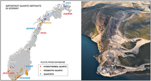
Norway stands as a primary producer of high-purity quartz, a fundamental raw material to produce silicon metal listed as a critical raw material by the European Union. The studied mine operated by ELKEM is in Tana, the Troms and Finnmark county in northern Norway (Figure 1). Elkem Tana mine is one of Europe’s largest quartzite mines, with annual production of one million tons. The production is carried out by drilling and blasting methods. The dilution of shale, the other main lithology in the mine, poses a significant challenge. Shale dilution adversely affects the quality of the quartzite, rendering it unsuitable for sale. As a result, this lower-quality quartzite is sent to waste rock dumps, leading to environmental effects, increased transportation and storage costs, and inefficient utilisation of the resources.

Figure 1. Elkem Tana quartzite mine.

Measurement while drilling (MWD) data has been routinely collected in the mine, as part of its digital transformation policy. It provides high-resolution information about the rock mass, offering a cost-effective alternative to conventional methods such as core drilling, geological mapping, and the analysis of drill cuttings [1]. In the studied mine, the collected MWD data has not been used as a decision-making tool yet. Various modelling techniques, including emerging machine learning (ML) models, have been deployed in open-pit and underground mines to extract valuable information from MWD. Leighton [2] modified blast design by considering the peaks in the MWD parameter, penetration rate, as an indication of weak zones. According to Segui and Higgins [3], MWD data may be utilised to enhance blast performance in mines. Regarding the data collected from MWD parameters, they suggested a different type and quantity of explosive can be utilised for each blast hole. Ghosh et al. [4], assessed the charge ability of the blast holes with drill monitoring data gathered from In-The-Hole (ITH) hammers. They calculated the fracturing parameter to get additional information about rock properties. Rodgers et al. [5] performed research on real-time assessment of unconfined compressive strength of rock while drilling a shaft utilising five monitored drilling parameters: torque, crowd, rotational speed, penetration rate, and bit diameter. Basarir [6] used MWD information from blast hole drilling machine to predict rock mass strength in an open pit lignite mine. Manzoor et al. [26] found that there is a strong correlation between fine and medium fragmented material with rock types classified using MWD data. This study aims at developing lithology prediction models using an emerging modelling algorithm, the Extreme Gradient Boosting (XGBOOST). Initially, a model (model #1) using a small-scale database composed of data from 10 boreholes was constructed. Geophysical measurements were conducted in the holes to label rock lithology as either quartzite or shale. MWD data was related to the labelled lithology using the model. The second model (model #2) was constructed using the expanded database by adding more data from 40 holes drilled in a production bench in the quartzite layer. More data was added to the second database through the inclusion of historical lidar face scans and corresponding MWD records. The third model (model #3) was constructed using the largest database. As in the usual case of earth sciences, the databases have different natures and challenges such as limited data and unbalanced data inclusion. Training models on datasets where the minority class is highly underrepresented often leads to classifiers that exhibit bias against the majority class, resulting in higher prediction accuracy for this class but poorer accuracy for the minority class. Rare cases or unbalanced class distributions are common in various real-world scenarios. Examples of such rare events in earth science include landslides, oil spills and hurricanes (Kubat et al. [24,25,29]). Dealing with these rare events challenges traditional methods of classification. However, it is concluded that XGBOOST is an effective algorithm in handling limited and unbalanced datasets. The performance of the models was evaluated using various classification metrics and the best performing model was selected. On the selected model, sensitivity analysis was conducted for model judgement and the parameters weighting assessment. The suggested model can be used as a practical tool for the mine to reduce shale dilution, minimise waste, and enhance the efficient use of the resources. By maximising resource utilisation and minimising waste, the model contributes to the efficient utilisation of mineral resources, promoting sustainable practices within the mining sector. This aligns with the Sustainable Development Goals (SDG) #12 set by the United Nations having the principal goal of achieving sustainable development by balancing economic growth with environmental protection and social responsibility.

The present study underscores an important caveat: its findings are tailored to the specific geological context in which it was conducted. While the insights gleaned from this research offer valuable guidance, it’s essential to recognise that every mine and ore deposit possesses its own distinct attributes and challenges. Consequently, the predictive models generated through this study may not be directly applicable to other mines or sites. Mining is inherently a complex interaction of geological and environmental factors, all of which contribute to the uniqueness of each site. From the composition of the ore to the geological formations surrounding the mine, numerous variables shape the mining process. Attempting to apply generalised models to diverse contexts can lead to inaccuracies and inefficiencies, potentially undermining the effectiveness of operations.

2. Field study

The field study involved a comprehensive approach that combined geophysical measurements in drill holes, field observations, and a review of historical face scans to label rock lithology and the collection of corresponding MWD data from drill holes.

Quartzite and shale are the two main lithologies in the mine. The quartzite appears in white to grey, brown, yellow, red, and pink colours, often with massive layers and occasional fractures. In contrast, the shale is presented in shades of grey, brown, and mostly black, with dry fractures and trace fossils. Radioactivity, particularly measurements of elements like potassium (K), thorium (Th), and uranium (U), also provides additional distinguishing characteristics, with the spectral gamma tool effectively differentiating between quartzite and shale.

In many earth science-related problems, the occurrences of events of interest are rare compared to the vast amount of normal or non-event data. Traditional statistical methods often struggle with such imbalanced datasets, where the rare events are overshadowed by the abundance of normal instances. However, machine learning techniques offer promising solutions to address this challenge. Three different databases were constructed through field studies for predictive model development to show the strength of modelling method selected modelling method in dealing with imbalances datasets.

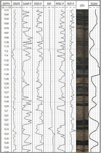
Database #1: This initial dataset was constructed using MWD and geophysical measurements from 10 drill holes strategically chosen in the mine. The geophysical measurements, including optical televiewer (OTV) and spectral gamma (SGAM) data, were employed to label the lithology passed through by each drill hole segment. SGAM measurement identifies the existence of radioactive material inside the borehole at each depth with the predefined sampling rate. The SGAM measurements include the amount of existing radioactive elements such as potassium (K), thorium (Th) and uranium (U). The spectral gamma tool measures the energy of the gamma emissions and counts the number of gamma emissions associated with each energy level. It gives quite efficient results in distinguishing quartzite and shale [7]. The OTV, which captures high-resolution images, is used to view each hole in 360 degrees.

Figure 2 presents OTV image and SGAM measurements with depth index for one of the boreholes. From the measurements it is possible to label each segment either quartzite (light grey in colour and low SGAM) or shale (black colour and high SGAM). The procedure was repeated for all holes and the database containing MWD data and labelled lithology was created.

Figure 2. SGAM measurements and OTV image for one borehole.

Database #2: Building upon Database #1, additional data from 40 blast holes drilled in a bench in quartzite layer (Figure 3) was incorporated to create Database #2.

Figure 3. Bench in quartzite layer.

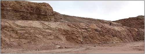
Database #3: Historical lidar radar face scans were reviewed to identify locations where blast holes passed through shale formations. These face scans visually revealed distinct layers of shale, white quartzite, and red quartzite. The contact line between shale and quartzite is indicated by the green line in Figure 4. MWD data belonging to the hole passing through that visible shale layer above the green contact line was extracted from the historical MWD archive. The new data was added to Database # 2 to create the largest database, Database #3.

Figure 4. Panoramic image from historical face scans showing shale, quartzite layers and contact line [28].

The MWD data included in Databases #1-#3 was recorded by the drill monitoring system of EPIROC – Smart Rock T40 drilling rig for each 5 cm intervals or so-called segments. The recorded parameters are; logging time, depth (metres), penetration rate (DRATE, m/min) at which the drill bit cuts through the rock mass, flush air pressure (FAP, bar) necessary to transport drill cuttings out of the borehole, percussion pressure (PERC-P, bar) emitted by the piston while pounding, feed pressure (FEED-P, bar) the amount of force required to lower the entire hammer, rotation pressure (ROT-P, bar) the amount of force required to lower the entire hammer and dampening pressure (DAMP-P, bar) the pressure that the drill rig absorbs to stop vibrations or unwanted movement inside the drill rig. The length of the 102 mm diameter boreholes ranged from 9 m to 23 m, resulting in varying numbers of data rows or segments per hole, ranging from 180 to 460.

By using multiple datasets with varying degrees of class imbalance, it is evaluated the robustness and generalisability of the XGBOOST model in different scenarios. Imbalanced datasets pose a significant challenge to traditional machine-learning algorithms. The diverse nature of these databases presented unique challenges, including limited data and unbalanced class distributions. In such datasets, the distribution of classes of interest is skewed, with one class significantly outnumbering the others. This can lead to biased models that prioritise the majority class, resulting in poor performance, especially when it comes to accurately predicting minority classes or rare events. These factors are taken into account during model development and evaluation, allowing a comprehensive evaluation of the model’s performance under various conditions and shedding light on the model’s ability to effectively handle imbalanced data.

3. Modelling

Machine learning (ML) serves as a powerful tool for building predictive models by leveraging available information to establish relationships between predictor and outcome variables. Similar to the other studies in the literature [8–10], the datasets created in the field study were divided into two subsets: a training dataset (comprising 80% of the data) used to train the model and a testing dataset (comprising 20% of the data) used to assess the trained model’s performance on unseen data.

Python programming [11], supported by the JupyterLab web-based user interface [12], and the scikit-learn package [13] was used to develop and fine-tune the models. In the training phase, k-fold cross-validation was used. The training phase included k-fold cross-validation, where the training dataset was randomly divided into k-folds. Of these, k-1 folds were used for model training, while the remaining fold was preserved for testing during training. This approach allowed the model to be updated k times of model parameter updates on various k-folds of data, reducing the risk of overfitting [14]. Overfitting occurs when a model learns to memorise training data rather than generalising it, leading to poor performance on unseen data. To deal with this issue in this study k-fold cross-validation method repeatedly training the model on different subsets of data and validating the unseen parts was used to ensure that the model does not become overspecialised for any subset of data. The used method learns patterns that are more likely to generalise to unseen data [15].

3.1. Data preprocessing

Before proceeding with the model development phase, the raw MWD data underwent preprocessing to filter out unrealistic and faulty data, which could potentially lead to misinterpretation. During drilling new rods are attached to the drilling string at the first 2.4 m and then at every 3.6 metres. Such pauses lead to some anomalies in the dataset. Thus, the data at these depths are removed from the dataset. After going through the filtering process, the datasets remain true to the integrity of the original data structure, ensuring that no deformation is triggered with a %10 to %15 change in mean and standard deviation values. The filtering process preserves the integrity of the data structure, ensuring that no important details are lost or misrepresented. Each observation in the datasets continues to accurately reflect the characteristics of the rock mass under study, including various geological features and environmental conditions. The study exclusively employs numerical-continuous values as inputs, conversely, the predicted lithology class represents a categorical variable, delineating distinct geological formations. Table 1 represents the summary statistics of three MWD datasets after rod change filtration. The table allows for a comprehensive comparison of the descriptive statistics across all three datasets, facilitating insights into the characteristics and distribution of each variable. It is anticipated that the DRATE will be lower in quartzites given that quartzite is characterised by its nature which is harder than shales. This is clearly seen in the average DRATE values presented in Table. As the quartzite ratio in the dataset increases, DRATE decreases, and the increase in the shale ratio corresponds to the increase in DRATE.

Table 1. Descriptive statistics of the three filtered datasets.

# of dataset		DRATE	PERC-P	FEED-P	FAP	ROT-P	DAMP-P
	Count	2684	2684	2684	2684	2684	2684
	Mean	1.51	184.16	48.67	6.45	56.50	58.86
	St. dev.	0.62	29.08	10.87	1.18	7.05	9.27
Dataset #1	Min	0.43	111.85	10.72	4.19	28.47	42.43
	25%	1.18	162.46	40.40	5.57	53.08	49.20
	50%	1.43	202.70	53.23	6.17	56.86	60.14
	75%	1.68	207.08	57.87	7.18	60.44	67.22
	Max	8.24	213.86	65.49	11.78	111.39	83.69
	Count	12810	12810	12810	12810	12810	12810
	Mean	1.28	189.87	52.15	5.87	52.56	62.18
	St. dev.	0.51	25.34	9.42	0.82	9.23	8.10
Dataset #2	Min	0.00	0.00	0.07	3.72	0.00	38.75
	25%	1.00	194.96	50.30	5.46	48.87	57.51
	50%	1.21	199.97	55.99	5.85	53.39	64.25
	75%	1.43	204.53	58.22	6.21	57.10	68.17
	Max	9.91	215.07	66.96	11.78	111.39	83.69
	Count	14163	14163	14163	14163	14163	14163
	Mean	1.32	187.16	50.94	5.76	53.28	61.11
	St. dev.	0.51	26.53	9.95	0.87	9.20	8.50
Dataset #3	Min	0.00	0.00	0.07	3.31	0.00	38.75
	25%	1.02	180.72	44.90	5.28	49.33	54.03
	50%	1.21	199.66	55.88	5.74	54.13	63.41
	75%	1.53	204.30	57.99	6.15	57.99	67.78
	Max	9.91	215.07	66.96	11.78	111.39	83.69

Following the filtering step, the data is labelled considering both the SGAM measurements and OTV images.

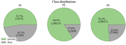
Datasets #1, #2 and #3 contain 2684, 12810, and 14,163 samples, respectively. Each sample represents five cm long segment in the borehole, the segment length was predefined by the selected sampling rate during the MWD data recording stage. Quartzite and shale distributions in the datasets differ as seen in the pie charts, in Figure 5. Quartzite and shale distributions are almost the same in the first dataset, whereas shale-to-quartzite ratios are approximately 1:5 and 1:3 in the second and third datasets, respectively. The datasets used in this study exhibited unbalanced class distributions, a common occurrence in geoscience-related problems. While various techniques such as synthetic minority over-sampling technique (SMOTE) [16], or generative adversarial nets (GANs) [17] can be employed to balance classes by generating synthetic data, it was decided to retain the original, unbalanced data for model generation. This choice allowed for a more realistic assessment of the modelling technique’s performance.

Figure 5. Quartzite and shale distributions in the datasets.

3.2. Extreme gradient boosting (XGBOOST) algorithm

The selected modelling algorithm for this study was the Extreme Gradient Boosting (XGBOOST). The algorithm was chosen for several reasons: its computational efficiency, ability to handle unbalanced datasets, and versatility in addressing both classification and regression problems. XGBOOST is an ensemble tree method and was created for the first time by Chen and He [18]. It is an implementation of gradient boosting by Friedman et al. [19]. It combines numerous weak learners to create a powerful learner by using decision trees as a base learner. The output of the base learners (i.e. trees) is used in the final prediction. XGBOOST repeatedly builds a collection of weak models, weighting each weak prediction in accordance with the effectiveness of the weak learner. Due to the parallel generation and processing of the boosted trees, it presents a trustworthy and quick model for various engineering simulations handling both classification and regression problems [20].

To gain a deeper understanding of how XGBOOST works, it’s essential to comprehend decision trees. Decision trees employ a series of nested yes/no questions to define decision boundaries. These trees are particularly effective when dealing with both numeric and ordinal variables. In a decision tree, the dataset is split into nodes based on specific variables, and the splitting algorithm examines potential splits at each node. The nodes become terminal nodes when most of the data within them belongs to a single class, at which point they are given a class label corresponding to the majority class.

In Figure 6, an example with a numeric variable (TI), an ordinal variable (PE), and outputs is given. It is clear that the linear model does not work well in the setting of boundaries [21].

Figure 6. Numeric, ordinal variables and outputs [21].

A decision tree for categorising the outputs mentioned in Figure 6 above is seen in Figure 7. The first node, or root, is divided based on the variable TI: situations for which TI > 5 follow the left branch and are all categorised as blue; cases for which TI < 5 travel to the right ‘child’ of the root node, where they are subject to further split tests. The splitting algorithm examines all the variables and potential splits at each new node. The nodes become ‘terminal’ nodes when most of the data entering a specific node belongs to a single class, at which point the node is no longer split and is given a class label corresponding to the majority class within it. To categorise a new observation, such as the white dot in Figure 7, one simply moves through the tree starting at the top (root), following the left branch when a split test condition is met and the right branch otherwise, until reaching a terminal node. The prediction is given as the terminal node’s class label [21].

Figure 7. An example for how decision tree works [21].

3.3. Performance metrics

The commonly used classification model performance metrics such as accuracy score, precision, recall and F1 score are calculated using the information from confusion matrix. Table 2 represents an example of a confusion matrix with two classes. Positive and negative classes are represented by 1 and 0, respectively. The diagonal values represent the number of true predictions, while the remaining values represent the number of false ones. The metrics consider the number of examples of a class that were correctly predicted to be positive (true positive), correctly predicted to be negative (true negative), and wrongly predicted classes (false negative or false positive) [22].

Table 2. Example confusion matrix with two classes [22].

Predicted Class	Actual Class
	Positive (1)	Negative (0)
Positive (1)	True Positive (TP)	False Positive (FP)
Negative (0)	False negative (FN)	True Negative (TN)

The formulas used for calculating performance indicators are given in Table 3. The overall correctness of predictions is measured by the accuracy. Precision measures the proportion of true positives to all positive predictions. Recall or sensitivity is used to measure the proportion of true positives among all actual positive instances. F1 score balances precision and recall, a high F1 score indicates that the model provides a good balance between precision and recall [22].

Table 3. Classification metrics and formulas [22].

Metric	Formula
Accuracy	(TN+TP)/(TN+FN+TP+TN)
Precision	TP/(TP+FP)
Recall	TP/(TP+FN)
False positive rate (FPR)	FP/(FP+TN)
F1 Score	(2(Precision×Recall)/(Precision+Recall))

Generally, the performance of a binary classification model on the positive class is illustrated in a graphic called as receiver operating characteristic (ROC) curve. An example ROC curve is shown in Figure 8. The model’s success is expressed by the calculation of the area under ROC curve (AUC-ROC). A classifier with a False Positive Rate (FPR) of 0 and a True Positive Rate (TPR) of 0 will generate a diagonal line if it lacks the ability to distinguish between positive and negative classifications. A diagonal line from the bottom left of the plot to the top right represents a model with no skill (random classifier) at each threshold and has an AUC-ROC of 0.5. The dashed line represents a model with perfect skill (ideal model). Lines A and B represent two different models with different skills. The success of these models lies between the random classifier and the ideal model [23].

Figure 8. An example ROC curve.

It might not be fair to use some of the performance indicators mentioned above for unbalanced datasets as in the case of many geoscience-related problems. When dealing with unbalanced datasets Precision-Recall (PR) curve is particularly useful. The area under PR curve (AUC-PR) provides an overall measure of a model’s ability to make correct positive predictions. An example PR curve is shown in Figure 9. The dashed line represents a model with perfect skill (ideal model). A curve that bows in the direction of the coordinate (1,1) is a good indicator of a good model. A horizontal line with precision will represent a no-skill classifier on the graph.

Figure 9. Example PR curve.

4. Results and discussion

The success of the XGBOOST algorithm is briefly compared with one of the traditional algorithms logistic regression. Logistic regression is a well-established and widely used statistical method for binary classification tasks, its performance may be limited in complex, nonlinear datasets such as those found in earth science. XGBOOST offers several advantages over logistic regression. Firstly, XGBOOST is capable of capturing complex relationships between input variables and output predictions through the use of decision trees, ensemble learning, and regularisation techniques. This allows XGBOOST to handle nonlinearity, interactions, and feature importance more effectively compared to logistic regression. The confusion matrices of the developed models for the test sets shown in Figures 10 and 11 were analysed to assess the models’ performance. In each model, shale, and quartzite lithologies were categorised as the positive and negative classes, respectively. The accuracy of each model on training and testing datasets is presented in Figure 12. XGBOOST algorithm for each dataset made more successful predictions in both the training and testing phases compared to the logistic regression model.

Figure 10. Confusion matrices of test data-XGBOOST models.

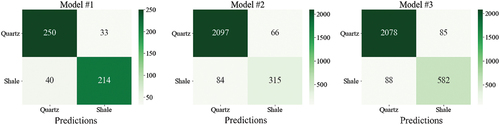
Figure 11. Confusion matrices of test data-logistic regression models.

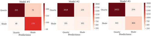
Figure 12. Accuracy of the XGBOOST (a) and logistic regression (b) models on train and test steps.

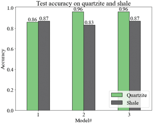
A more in-depth analysis of the XGBOOST model was then conducted to examine the success of the model on each class. Unbalanced class distributions had a minimal effect on the individual lithology prediction accuracy of the classification models #2 and #3 (Figure 13). Given shale’s detrimental impact on the ore quality, correctly predicting positive class or shale layers held a priority. The models’ success on the second and third datasets demonstrated that the prediction of shale, despite class imbalance, remained robust against the logistic regression model.

Figure 13. Accuracy of the XGBOOST models on test data based on classes.

Figure 14 shows ROC and PR curves used to visualise model success. ROC curve efficiently assesses models for balanced datasets however it may give an over-positive impression of a model’s effectiveness in the event of very unbalanced data sets. PR curves provide a more accurate representation when faced with highly imbalanced data sets. A big area under PR curve denotes both high recall and high precision [27].

Figure 14. ROC curve, UAC-ROC, PR curve, UAC-PR from models #1, #2 and #3.

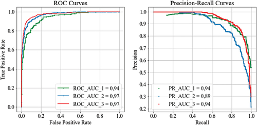
In Table 4, essential metrics including AUC-ROC, AUC-PR, precision, recall, and F1 score are presented. Model #3 exhibits the higher AUC-ROC than Model #1, highest precision and F1 score while maintaining a recall rate identical to that of Model #1. Given the paramount importance of correctly predicting shale, model #3’s high AUC-ROC, highest precision, and F1 score indication of balance between precision and recall, makes model #3 the preferred choice.

Table 4. Performance metrics of the models.

Model #	AUC-ROC	AUC-PR	Precision	Recall	F1 Score
1	0.94	0.94	0.84	0.87	0.85
2	0.97	0.89	0.79	0.83	0.81
3	0.97	0.94	0.87	0.87	0.89

Sensitivity analysis was conducted on the selected model (model #3), to find out the most significant MWD parameters or ‘discriminative features’ that the model used frequently when making predictions. The importance of MWD parameters for the model are shown in Figure 15. The most influential parameter is DAMP-P (29%) followed by FAP (21%) and DRATE (20%).

Figure 15. Feature importance of MWD parameters for the selected model #3.

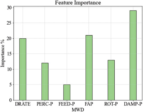
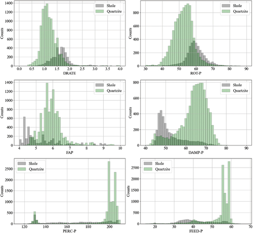
To justify the results of sensitivity analysis and thereby the selected model, the distributions of MWD parameters for shale and quartzite lithologies shown in Figure 16 are investigated. When the distributions of the most significant parameters or discriminative features such as DAMP-P, FAP and DRATE are considered, the clear difference between the modes or major modes of shale and quartzite distributions is noticed. Whereas the larger overlapping area is observed for other variables such as ROT-P, PERC-P and FEED-P. Although there are also intersection areas for DAMP-P, FAP and DRATE, there is a sharper difference between the areas where the data is concentrated for quartzite and shale. Moreover, the difference seems to be proportional to the significance of the parameters. For instance, the relatively lower dampening pressure (DAMP-P) and flush air pressure (FAP) observed in shale lithology is attributed to its relatively lower density and strength in comparison to quartzite. Additionally, the higher penetration rate (DRATE) associated with shale is indicative of its softer and less resistant nature compared to the stronger quartzite. These distinctions in MWD parameters directly correspond to the contrasting physical properties of the two lithologies and are integral to the accurate classification achieved by the model.

Figure 16. MWD data distribution based on the lithologies.

5. Conclusion

The developed lithology prediction models using the Extreme Gradient Boosting (XGBOOST) algorithm, based on measurement while drilling (MWD) data, have yielded promising results. Three different models were constructed using different databases and the best-performing model was selected considering performance metrics. The suggested model has demonstrated its effectiveness in addressing the specific challenges of the mine, where shale dilution affects the quality of produced ore quartzite. Through thorough sensitivity analysis, key MWD parameters playing a critical role in lithology prediction were assessed. It is concluded that the parameters, having distinctive differences between quartzite and shale, have been frequently used by the modelling algorithm in making accurate predictions. The suggested model can be used for reducing shale dilution, enhancing quartzite quality, and minimising waste. Therefore, the use of the model contributes to the sustainable and efficient management of mineral resources as suggested by the United Nations Sustainable Development Goal #12, focusing on the efficient production of resources.

Thanks to its ability to handle sparse and unbalanced data, XGBOOST offers a powerful solution for mining companies struggling with the complexity of geological datasets. Its robustness, flexibility, and ability to handle imbalanced datasets make it a valuable tool for researchers in earth sciences seeking to build accurate predictive models from unbalanced data. By accurately predicting lithology classes and identifying areas of potential shale dilution, the model empowers mining engineers and operators to make informed decisions that minimise waste and maximise resource use. Moreover, the proposed model serves as more than just a predictive tool; It represents a strategic asset to promote sustainable practices in the mining industry. The model enables proactive measures to reduce shale dilution and optimise resource extraction, contributing to the efficient use of natural resources and reducing environmental impact. As mentioned earlier, although the developed model cannot be used directly, the presented approach can be applied by different mines to achieve the overall goal of maximising resource utilisation. Integration of such advanced modelling approaches, as exemplified in this study, promises to revolutionise resource optimisation and environmental sustainability in the mining industry.

Using a machine learning framework to predict lithology classes from numerical inputs, this work advances the field of earth sciences by offering a data-driven approach to lithological interpretation. Additionally, the use of numerical-continuous values as input highlights the interdisciplinary nature of the research, bridging the gap between quantitative data analysis and geological interpretation. Implementing spatial interpolation techniques could help extrapolate lithology predictions between borehole locations, providing a more continuous representation of subsurface geology. Methods such as kriging or inverse distance weighting could be explored to fill in gaps between data points and generate seamless lithology maps. The data points or predicted lithologies by the improved XGB model can be used as input for spatial interpolation techniques for creating the overall geological model representing the mine field or part of it.

Computer code availability

Data sharing not applicable. However, the python script used in the training and testing stage of the models can be found at https://github.com/ozgeakyldz/.

Author’s contribution

Ozge Akyildiz 1: The author was involved in data collection and analysis, developing ideas, their interpretation and implementation as well as preparation of the manuscript.

Hakan Basarir 2: The author was involved in data collection and analysis, developing ideas, their interpretation and implementation, writing and revising of the manuscript.

Steinar Løve Ellefmo 3: The author made significant contributions to developing ideas and their [29]implementation and revising the manuscript.

All authors give the final approval of the manuscript to be submitted and any revised version of it.

Acknowledgments

This research is the outcome of a collaboration between the Geoscience and Petroleum Department, Norwegian University of Science and Technology (NTNU) and ELKEM ASA Tana. The authors acknowledge ELKEM ASA Tana for the data support and their valuable input and discussions.

Disclosure statement

No potential conflict of interest was reported by the author(s).

References

- H. Schunnesson, RQD predictions based on drill performance parameters, Tunnell. Undergr. Space Technol. 11 (1996), pp. 345–351. https://linkinghub.elsevier.com/retrieve/pii/0886779896000247.
- J. Leighton, Development of a Correlation Between Rotary Drill Performance and Controlled Blasting Powder Factors, University of British Columbia, Canada, (1982).
- J.B. Segui and M. Higgins, Blast design using measurement while drilling parameters, Int. J. Blast. Fragment. 6 (2002), pp. 287–299. doi:10.1076/frag.6.3.287.14052.
- R. Ghosh, A. Gustafson, and H. Schunnesson, Development of a geo-mechanical model for chargeability assessment of borehole using drill monitoring technique, Int. J. Rock Mech. Min. Sci. 109 (2018), pp. 9–18. doi:10.1016/j.ijrmms.2018.06.015.
- M. Rodgers, M. McVay, and D. Horhota, Assessment of rock strength from measuring while drilling shafts in Florida limestone, Can. Geotech. J. 55 (8) (2017), pp. 1154–1167. doi:10.1139/cgj-2017-0321.
- H. Basarir, Prediction of rock mass P wave velocity using blasthole drilling information, Int. J. Min. Reclam. Environ. 33 (1) (2019), pp. 61–74. https://www.tandfonline.com/doi/full/10.1080/17480930.17482017.11354960.
- D.V. Ellis and J.M. Singer, Well Logging for Earth Scientists, Springer, The Netherlands, 2007.
- M.A. Grima, P.A. Bruines, and P.N.W. Verhoef, Modeling tunnel boring machine performance by neuro-fuzzy methods, Tunnelling Underground Space Technology. 15 (3) (2000), pp. 259–269. doi:10.1016/S0886-7798(00)00055-9.
- H. Basarir, J. Wesseloo, and A. Karrech, The use of soft computing methods for the prediction of rock properties based on measurement while drilling data, Deep Mining 2017: Eighth International Conference on Deep and High Stress Mining, Perth, WA, (2017), pp. 537–551.
- A. Verma and T.N. Singh, A neuro-fuzzy approach for prediction of longitudinal wave velocity, Neural. Comput. Appl. 22 (7–8) (2013), pp. 1685–1693. doi:10.1007/s00521-012-0817-5.
- G.V. Rossum and F.L. Drake, Python 3 reference manual, CreateSpace, 100 enterprise way, suite A200, Scotts Valley, CA, 2009.
- T. Kluyver, B. Ragan-Kelley, and F. Pérez, Jupyter notebooks – a publishing format for reproducible computational workflows, 20th International Conference on Electronic Publishing Gothingen, Germany, (2016).
- F. Pedregosa, G. Varoquaux, and A. Gramfort, Scikit-learn: Machine learning in Python, J. Mach. Learn. Res. 12 (2011), pp. 2825–2830.
- E. Sadrossadat, H. Basarir, and A. Karrech, An engineered ML model for prediction of the compressive strength of Eco-SCC based on type and proportions of materials, Cleaner Mater. 4 (2022), pp. 100072. doi:10.1016/j.clema.2022.100072.
- G. James, D. Witten, T. Hastie, R. Tibshirani, and J. Taylor, An Introduction to Statistical Learning with Applications in Python, Switzerland: Springer, (2023).
- N.V. Chawla, K.W. Bowyer, and L.O. Hall, SMOTE: Synthetic minority over-sampling technique, J. Artif. Intell. Res. 16 (2002), pp. 321–357. doi:10.1613/jair.953.
- I.J. Goodfellow, J. Pouget-Abadie, and M. Mirza, Generative adversarial nets, NIPS’14: Proceedings of the 27th International Conference on Neural Information Processing Systems Vol 2 Montreal, Canada, (2014), pp. 2672–2680.
- T. Chen and T. He 13 August , XGBoost: A Scalable Tree Boosting System KDD ‘16: Proceedings of the 22nd ACM SIGKDD International Conference on Knowledge Discovery and Data Mining (2016), pp. 785–794. doi:10.1145/2939672.2939785.
- J. Friedman, T. Hastie, and R. Tibshirani, Additive logistic regression: A statistical view of boosting, Ann. Statist. 28 (2) (2000), pp. 337–407. doi:10.1214/aos/1016218223.
- J. Zhou, E. Li, and M. Wang, Feasibility of stochastic gradient boosting approach for evaluating seismic liquefaction potential based on SPT and CPT case histories, J. Perform. Constr. Facil. 33 (3) (2019), doi:10.1061/(ASCE)CF.1943-5509.0001292.
- G. Seni and A. Elder, Ensemble Methods in Data Mining: Through Combining Predictions, Morgan & Claypool Publishers, (2010).
- M. Sokolova and G. Lapalme, A systematic analysis of performance measures for classification tasks, Inf. Proc. Manag. 45 (4) (2009), pp. 427–437. doi:10.1016/j.ipm.2009.03.002.
- P. Branco, L. Torgo, and R. Ribeiro, A survey of predictive modelling on imbalanced domains ACM Computing Surveys 49 (2) (2016), pp. 1–50.
- Trafalis, T.B., Ince, H., Richman, M.B. Tornado Detection with Support Vector Machines. Sloot, P.M.A., Abramson, D., Bogdanov, A.V., Gorbachev, Y.E., Dongarra, J.J., Zomaya, A.Y. eds, Computational Science — ICCS 2003. ICCS 2003. Lecture Notes in Computer Science, vol 2660, Springer, Berlin, Heidelberg. (2003). https://doi.org/10.1007/3-540-44864-0_30
- Kubat M, Holte R C and Matwin S. (1998). Machine Learning, 30(2/3), 195–215. doi:10.1023/A:1007452223027
- Danielsson M, Söderström E, Schunnesson H, Gustafson A, Fredriksson H, Johansson D and Manzoor S. (2022). Predicting rock fragmentation based on drill monitoring: A case study from Malmberget mine, Sweden, J. S. Afr. Inst. Min. Metall., 122(3), 1–11. doi:10.17159/2411-9717/1587/2022
- H. He and E.A. Garcia, Learning from imbalanced data, IEEE Trans. Knowl. Data Eng. 21 (9) (2009), pp. 1263–1284. doi:10.1109/TKDE.2008.239.
- Minnaard, Cornelis (Koen) W.). (2022). 4D Geomodelling using Lidar scans and MWD data analysis, Master Thesis. Trondheim, Norway: Departmnet of Geosceince and petroleum, NTNU.
- Van Den Eeckhaut M, Hervás J, Jaedicke C, Malet J, Montanarella L and Nadim F. (2012). Statistical modelling of Europe-wide landslide susceptibility using limited landslide inventory data, Landslides. 9(3), 357–369. doi:10.1007/s10346-011-0299-z