Influence of water level duration on dike breach triggering, focusing on system behaviour hazard analyses in lowland rivers

ABSTRACT

Hazard analysis is a crucial step in flood risk management, and for large rivers, the effects of breaches need to be taken into account. Hazard analyses that incorporate this overall “system behaviour” have become increasingly popular in flood risk assessment. Methods to perform such analyses often focus on high water levels as a trigger for dike breaching. However, the duration of high water levels is known to be another important failure criterion. This study aims to investigate the effect of including this duration dependency in system behaviour analyses, using a computational framework in which two dike breach triggering methods are compared. The first triggers dike breaches based on water levels, and the second one based on both water-level and duration. The comparison is made for the Dutch Rhine system, where the dike failure probabilities are assumed to conform to the new Dutch standards of protection. The results show that including the duration as a breach triggering variable has an effect on the hydraulic loads and overall behaviour in the system, therefore influencing the risk. Although further work is required to fully understand the potential impact, the study suggests that including this duration dependency is important for future hazard risk analyses.

KEYWORDS:

• System behaviour
• dike breaches
• protection standards

1. Introduction

Risk analysis is vital for the flood risk management of lowland river systems. It requires the analysis of hazard, exposure and vulnerability at a system level (Vorogushyn et al. 2017). To assess hazards, extreme value analysis of peak discharges is often used, from which flood frequency distributions can be generated. However, as noted by Apel, Merz, and Thieken (2009), the extrapolation to extreme events used in this analysis may fail to consider processes not present in recorded data, such as out-of-bank flows. Furthermore, extreme value analysis is applicable only to the location from which the observations are drawn, and cannot be applied to an entire system. Due to these deficiencies, system behaviour analyses have become increasingly popular in flood hazard estimation.

Hydrodynamic system behaviour considers the behaviour of the river system when out-of-bank flows are included, and is most often used in the estimation of extreme flows in low-land or delta river systems. The concept has, has in recent literature, been called “river system behaviour” (van Mierlo et al. 2007), “load interdependencies” (Klerk 2013; De Bruijn, Diermanse, and Beckers 2014; Dupuits et al. 2016) or simply “system behaviour” (Bachmann et al. 2013). Various studies (including those mentioned above) have demonstrated its importance in the Netherlands (De Bruijn, Diermanse, and Beckers 2014, 2016), and its relevance internationally has grown with studies in Germany (Vorogushyn et al. 2010; Falter et al. 2016), U.S.A (Dunn, Baker, and Fleming 2016) and Japan (Assteerawatt et al. 2016).

Studies of this type are often in relation to protected systems, where out-of-bank flows are primarily due to defence failures such as dike breaching. The temporal and spatial occurrence of dike breaches are highly uncertain and therefore probabilistic approaches to assess flood risk have been proposed by Apel, Merz, and Thieken (2009), Vorogushyn et al. (2010), De Bruijn, Diermanse, and Beckers (2014) and van Mierlo et al. (2007) amongst others. In each of these approaches, a Monte Carlo framework is used to sample variables such as loads, dike strengths and potential impacts for various locations on the river. Hydrodynamic simulations of a schematised area are then run multiple times and output variables (such as hydraulic loads, damages and system risks), can be inferred from the results. In these frameworks, sampled dike strengths will determine the conditions under which a dike breach is initiated or “triggered” in a simulation. The geotechnical complexity of this breach triggering and growth process usually requires a number of simplifications to be made.

One common simplification is to assume the triggering of a dike breach is due to water level alone, as done by Apel, Merz, and Thieken (2009), De Bruijn et al. (2016), Assteerawatt et al. (2016) and various others. The prevalence of this approach is partly due to the availability of “fragility curves” in many countries, which relate water level to probability of failure for a dike section, according to various failure mechanisms. A consequence of using water level from the curves as a breaching trigger is that breaching within a simulation can only occur before (or directly at), the peak of the floodwave. Although this approach is reasonable for overtopping, other dominant failure mechanisms such as piping and macrostability have been shown to have a strong dependency on the duration of the floodwave (i.e. the period of time the water level is above certain thresholds) as well as the water level itself.

This paper attempts to investigate the effect of floodwave duration in flood hazard analyses that include system behaviour, for the case study of the lower Rhine River in the Netherlands. The paper starts with a short review of existing system behaviour approaches and their application to the lower Rhine, as well as an overview of the mechanics of breaching. The methodology, results and conclusions are given in the proceeding sections.

2. Existing approaches

2.1. System behaviour

The studies on system behaviour mentioned above are primarily academic, and rarely used directly in Flood Risk Management (FRM), policy making. One of the main reasons for this is the difficulty in validating the analyses against the extreme events that they attempt to model. In the Netherlands, the newly introduced national risk standards (Kok et al. 2017) require flood fatality to be assessed at a national level. This policy has precipitated more detailed studies that can account for assessments at the national scale, and thus system behaviour analyses have become more relevant.

An assessment of the expected hydraulic loads coming into the Netherlands from the Rhine and Meuse is given by the “Generator of Rainfall and Discharge Extremes” (GRADE, Hegnauer et al. 2014). This study is an example of accounting for system behaviour, as the distributions of hydraulic variables for the Rhine resulting from this study (such as water level and discharge) take into account potential dike breaches upstream of the Dutch border. However, these breaches were considered in a deterministic way, occurring when certain water level thresholds related to overtopping were surpassed. Despite this simplification, the discharge and wave-shape distributions have been used in both legal policies and research on the Dutch Rhine, for example in the “Legal safety assessment 2017” (Slomp 2016).

The VNK2 project (Jongejan et al. 2011) gives quantitative risk estimates for each dike ring within the Netherlands, accounting for uncertainties relating to loading conditions, resistances, and physical models. Within the VNK2 project, sections of dike on the dikerings were defined in such a way that breaches anywhere along these sections are likely to cause similar inundation extents. However, the possibility of hydraulic system behaviour between the dike rings was not accounted for.

System behaviour research related to specific regions of dikerings in the Netherlands has been performed by Courage et al. (2013) and Klerk (2013), whereas analyses for simplified/hypothetical dikerings have been done by van Mierlo et al. (2007) and Dupuits et al. (2016). For the downstream boundary conditions in the Rhine delta, sea level distributions that include tidal variability have been used in system behaviour research by Diermanse et al. (2014). National-scale system behaviour analyses for the Netherlands have been applied to flood fatality risk (De Bruijn, Diermanse, and Beckers 2014), and to hydrodynamic behaviour (De Bruijn et al. 2016). However, these studies assumed breach triggering based on high water levels alone. As explained below, this simplification is unrealistic in relation to known breaching mechanisms.

2.2. Dike failure

The system behaviour studies mentioned above all utilise the concept of the reliability or limit-state equation; Z = R – S. Failure is said to occur when Z < 0, i.e. when the load or solicitation, (S) is greater than the strength or resistance, (R). In the case of a dike, the resistance is related to its composition and geometry whereas the loads relate to the hydraulic variables such as water-level, duration and discharge. For probabilistic failure analyses, both the strength and load variables are given in terms of distributions of these variables.

Distributions of dike strength are usually expressed in terms of their failure probability according to various mechanisms. A non-exhaustive list of failure mechanisms including liquefaction and collision is proposed by Vrijling (2001), and this is reduced to the principle mechanisms of overtopping, piping, slope failure and erosion by van Mierlo et al. (2003). Of these mechanisms, slope erosion and inner and outer slope failure are often grouped under the title macro-stability, leading to the system behaviour analysis of De Bruijn, Diermanse, and Beckers (2014) which focuses on piping, overtopping and macrostability. A dependence on the water level duration for each of these mechanisms is described by Sellmeijer et al. (2011), (piping), Van, Koelewijn, and Barends (2005), (macrostability) and Vorogushyn et al. (2010), (overtopping). Van et al. noted significant movement of a test dike after being exerted to high pore pressures for about two days, while Sellmeijer et al. observed critical heads leading to piping failure in a test dike after effects after 30–60 h. The full geotechnics of these mechanisms are not described here, but more complete details are available in the provided references as well as overviews by Vorogushyn, Merz, and Apel (2009), Steenbergen et al. (2004), Vrouwenvelder et al. (2010) and others.

These studies demonstrate that sustained water levels impact breaching probability and will, therefore, affect system behaviour analyses as described above. However, the models describing failure in this literature require detailed data inputs and are often technically complex, thus making them difficult to apply at a system level. A method to include a simplified duration dependency in a system behaviour analysis has been implemented by Vorogushyn et al. (2010), but still requires extensive geotechnical knowledge, and cannot be applied to the currently available data for the Dutch dike system. A system behaviour analysis that includes water level duration as a variable for breach triggering has not been performed for the Netherlands, and an objective of this study is to determine its effects on the hydrodynamic system behaviour and potential flood hazards on the Rhine.

3. Methodology and application

3.1. Computational framework

The presented research compares two dike-breach triggering methods for a hydrodynamic system behaviour analysis, using the Rhine case study. The comparison uses the concept of the reliability equation to trigger dike breaches probabilistically, where “S” is the distributions of hydraulic loads (peak discharge and wave-shape), and “R” is the distributions of dike strengths. These distributions are sampled in a Monte Carlo framework, and the resulting values are used as inputs to a hydrodynamic simulation of the system. The hydraulic output variables of interest from each simulation (such as water level and discharge) are combined into distributions based on the original input probabilities taken from the sampled values. The probabilistic framework for modelling each scenario has been adapted from De Bruijn, Diermanse, and Beckers (2014), and is given in Figure 1.

Figure 1. Probabilistic framework schematisation.

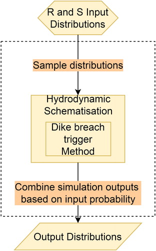
For the loads, S, the discharges at the upstream boundary are sampled using an importance sampling procedure giving preference to higher discharges, whereas the wave-shape and dike strengths are sampled using crude Monte Carlo sampling. In all tested implementations of this framework (termed scenarios), the input load distributions are the same. The dike strengths, R, are distributions of failure probability that relate to either water level or both water level and duration of exceedance of that water level. These two strength distributions have been termed “fragility curves” and “fragility surfaces” respectively, and “fragility functions” collectively. Their formation is described for the specific case-study below.

The process given in Figure 1 is repeated for three system behaviour scenarios. In scenario 0, system behaviour is not implemented (i.e. no out of bank flow occurs), and this is used to gauge the effect of the system behaviour scenarios. The frequency of breaching that would have occurred using both fragility curves and surfaces are recorded in scenario 0. In scenario 1 and 2, breaches are simulated and thus affect the river discharges. In all scenarios, the fragility functions are adjusted to ensure the resulting failure probabilities correspond to the probabilities required in the new protection standards when system behaviour is not considered.

3.2. Application to lower Rhine River

The presented case study area is the lower Rhine region along its three branches in the Netherlands; the Waal, the Nederrijn/Lek and the IJssel. The study is delimited upstream at Lobith on the German border, a location for which for which data is available for the distribution of hydraulic variables. The flow in the system is heavily dominated by the upstream flow, and therefore smaller inflows within the Netherlands are not considered. The river network is almost completely defended with dikes employing different protection standards. Tidal effects on the Lek and Waal (or Merwede as it is called downstream) are observed as far upstream as Nieuwegein and Gorinchem respectively but considered dominant downstream of Dordrecht and Rotterdam. For this reason, these latter locations delimit the case-study downstream; along with the IJsselmeer Lake (see Figure 2). The results at four locations of interest were chosen to illustrate the overall behaviour, and are labelled in Figure 2. The labels refer to a naming convention which describes the breach location on the branch, (Rhine, Pannerden Canal, Waal, Nederrijn/Lek or IJssel; R, P, W, L, or I, respectively). For example, “W2_r” is the second breach location on the Waal going downstream, and the breach is located on the right-hand side. The location of all breaches is given in Appendix 1.

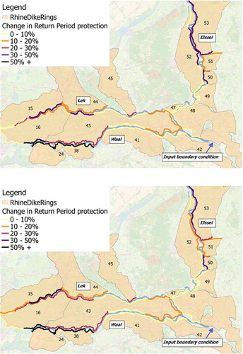
Figure 2. Top left map show case study location within the Netherlands. Indicated on larger map are the breach locations including the ones analysed in detail, as well as dike rings, river branches and the protection standards (failure probabilities of the embankment) associated with each dike trajectory.

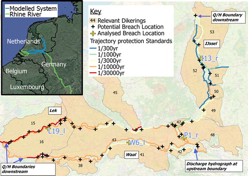
The case-study was modelled as a 1D Sobek3 schematisation, adapted from a benchmarked model developed for Rijkswaterstaat. Sixty-two predetermined breach locations were included to represent sections of dike as shown in Figure 2. These sections are based on a sub-discretisation of the dike “trajecten” or trajectories, for which protection standards are described by Dutch law (Slomp 2016). Given these trajectory protection standards, the design failure probabilities for each dike breach section can be estimated, by assuming every metre embankment contributes equally to the overall failure probability of the trajectory section.

Within the Sobek model, each breach location is schematised as a weir that flows to a reservoir that represents the capacity of the adjacent dike-ring (see Figure 2). In scenarios where system behaviour is implemented, the weir is triggered by exceedance of the sampled water level threshold or water level-duration threshold. If a breach is triggered, it will start to grow in length and depth according to the Verheij and van der Knaap (2002), breach growth formula, using default parameters (Appendix 2). In the model, water will then flow from the river through the breach into the dike-ring which means the river discharge downstream is reduced.

3.3. Hydraulic loads

The principal load is the river inflow coming from Germany, schematised as a discharge hydrograph boundary condition at Lobith, near the Dutch-German border, (see Figure 2). This hydrograph is generated by combining discharge peak and wave-shape values sampled from distributions at this location, taken from GRADE (Hegnauer et al. 2014). GRADE uses a combination of models to derive these distributions, such as a weather generator, a hydrological model and a hydraulic model. Different wave-shape distributions are assigned to hydrographs according to their peak value in the study, and these distributions were maintained for the present study, Figure 3. The downstream boundary conditions on all three branches were modelled using discharge–water levels (Q–H) relationships, meaning no tidal effects are considered. Given the focus of the study on dike-breaching mechanisms in system behaviour, this simplification was considered acceptable.

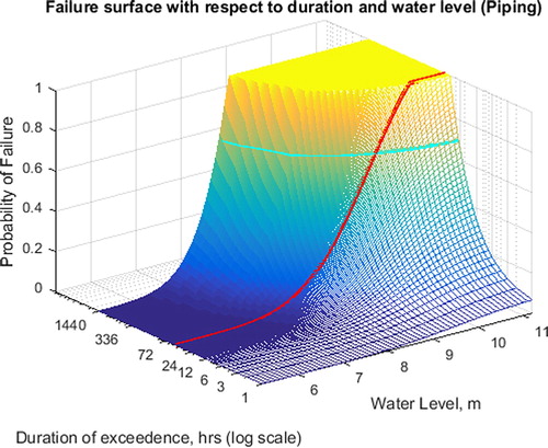
Figure 3. Example fragility surface for piping mechanism. Line in red shows original fragility curve, for which a duration of 48 h is considered most applicable by the experts. The cyan line shows the resulting threshold due to a sampling value of .7.

3.4. Dike strengths/resistance

In the present study, breaches occur when the river water levels (scenario 1), or river water level durations (scenario 2), surpass a threshold. Recently developed fragility curve for overtopping, piping and macrostability (Levelt et al. 2017) are used as the basis for those thresholds in both scenarios. These curves have been generated for small dike sections on the entire Rhine/Maas system, and were combined analytically to represent the breach locations given in Figure 2, assuming independence between the constituent curves. The standard deviations of these curves were maintained, but the mean values were adjusted so that failure probabilities in scenario 0 (without system behaviour) conform to the new protection standards. This constraint ensures the inclusion of water level duration as a breaching criterion does not severely affect the overall failure probability of the system, instead allowing for changes in system behaviour effects become apparent, such as breaching characteristics. This adjustment is done using a method similar to that described by De Bruijn, Diermanse, and Beckers (2014). The design probabilities per location and calculated probabilities are given in Appendix 1.

In scenario 1, sampled probabilities are transformed into threshold water levels using the fragility curves, and the lowest water level is used as the threshold for failure at that location. In scenario 2, breaching occurs due to a combination of water-level and the duration of time that level is exceeded in a simulation. The duration of exceedance of water levels was, therefore, added as a second variable to the fragility curves creating the example fragility surface shown in Figure 3. Sampled probabilities applied to this surface give an incremental range of water levels and associated exceedance durations for which failure would occur according to that probability. At each location, the ranges resulting from each mechanism were combined using the smallest duration for the incremental water level height, resulting in a single failure criterion.

To include the duration as a dependent variable in these surfaces, adjustment factors for the fragility curves for certain durations of water levels were elicited via the opinion of three dike failure experts. These values and the averages that were used are given in Table 1. The factors describe how the curve probabilities should be increased/decreased based on the durations. For example, a factor of .5 halves the probabilities described by the fragility curves for the corresponding duration, signifying the expert believes the fragility curves over-estimate the risk at this duration. Interpolating between these estimates creates surfaces similar to that shown below. This process was carried out for each breach mechanism and location in the model. Sampling values from each of the curves for a simulated event lead to the relationship between duration and water level for which failure would occur, as seen in the cyan line in Figure 3. As with the fragility curves, these surfaces were then adjusted to conform to the new protection standards. The original and adjusted curve data is given in Appendix 3.

Table 1. Factors to adjust fragility curves for certain durations, as suggested by three different dike fragility experts, and overall averages.

Expert	1 h	24 h	168 h	720 h
Overtopping
A	0.005	0.2	0.8	0.9
B	0.1	1.3	2	2
C	1	10	50	50
Average	0.37	3.83	17.6	17.63
Piping
A	0.0005	0.05	0.8	0.9
B	0.2	1	2	2.5
C	0.01	1	10	20
Average	0.07	0.68	4.27	7.8
Macrostability
A	0.02	0.1	0.6	0.9
B	0.7	1.3	1.8	2
C	0.01	1	10	20
Average	0.24	0.8	4.13	7.63

It can be seen that all experts agree that the existing fragility curves represent the uncertainty for some duration, as a factor of 1 lies within each range given, and this was generally the basis of the experts’ decision making. The steady increases in the factors with respect to duration show a clear dependency on this variable. However, the factors offered by experts differ greatly. This could be for numerous reasons, such as prior knowledge of the development of the curves, or a difference between understanding of the terms “breaching” and “failure”.

The sensitivity of these factors on the hydraulic results was not considered due to the demonstrative nature of this work, However, it should be noted that using these factors for scenario 2 factors represent a best-estimate between the extremes represented by scenario 0 (no system behaviour) and scenario 1 (system behaviour based on water level alone). In scenario 1, embankments will fail in the rising limb of the floodwave, ensuring large breach volumes are removed the river system. In scenario 2, no breach volumes are removed from the river. Accounting for duration in scenario 2, embankments may also fail later which reduces the effect of the breach downstream.

While the use of different factors likely has an effect on the specific breaching estimates quantified in the results, it is recommended that a more structured expert judgement analysis elicit duration dependency be prioritised over sensitivity analyses for future studies.

3.5. Probabilistic analysis

Using the load and strength distribution probabilities described above, multiple simulations were run, and output variables of interest were recorded to compute probability distributions. In order to track and compute the input and output variables used in each simulation, and their associated probabilities, the Probabilistic Toolkit^© was used to “wrap” the simulations. This tool collected and analysed the output data, referencing the input probabilities that had been used in that simulation. Sample probabilities were generated using importance sampling based around 16,000 m³/s for the discharge, with a maximum of 20,000 m³/s. The dike strengths and wave shapes were sampled with crude Monte Carlo sampling. Fifteen thousand simulations were run for each scenario, based on the convergence of the breaching failure probabilities. The scenarios were analysed in terms of hydraulic loads in the system, failure probabilities, and breaching data per location. The outcomes are discussed in the following section.

4. Results and discussion

4.1. Hydraulic loads

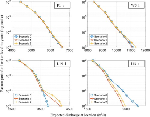
The calculated return period water levels for the four selected locations of interest are compared in Figure 4. It is immediately apparent that system behaviour leads to a reduction in the water levels, which is to be expected at all downstream locations, with the difference only being observed at higher return periods. Although it is small, a reduction of this impact is seen in scenario 2, due to the lower abstraction from the river when failure occurs after the peak of the flood wave. At less extreme flows, scenario 2 conforms more closely to scenario 0. In this scenario, breaches still occur, but many of the breaches are coming late in the flood wave, reducing the impact of system behaviour. At location I13_r, the impact of system behaviour is observed at smaller return periods, and is greater than the other locations, but it should be noted that the scales on the x-axis are different for all locations. This larger impact is principally due to the lower protection standards on the IJssel.

Figure 4. Return period water levels for Scenarios 0, 1 and 2, at locations P1_r, W6_l, L19_1 and I13_l. These locations can be seen on a map in Figure 2. Note that the x-axis scales are not the same per location. Scenarios 0, 1 and 2 represent no system behaviour, system behaviour dependent on water level and system behaviour dependent on water level and duration, respectively.

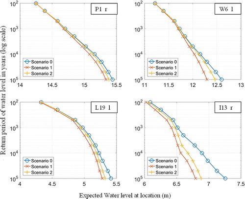
An interesting aspect of system behaviour is noted when the corresponding discharges at these locations are assessed. At location “P1_r” the difference in discharges is negligible for all scenarios, despite having breach locations upstream of that location. This is due to a “drawdown” effect of breaches downstream causing a water level gradient and pulling water downstream, and a similar effect is seen at location W6_l. An extreme example of this is observed at L19_l, where the large breach volume that occurs at that location causes higher peak discharges than the scenario without system behaviour. This effect has been observed by Kiss, Fehérváry, and Fiala (2015), who noted increases in water stream slope and power in river stretches upstream of breaches. In this instance, scenario 2 increases this effect, which is probably due to the increased water levels experienced at this location, which cause higher drawdowns and therefore larger discharges. The severity of this effect may be due to the simplification of using a 1D reservoir to represent the floodplain behind the breach, but the underlying principal behind it will still occur even with a more advanced schematisation. At location I13_r on the IJssel the reduction in discharge more closely corresponds to the water level distribution, and as with the water levels, breach triggering using duration as a variable mitigates the effect of system behaviour.

4.2. Failure probabilities

The relative change in trajectory failure probability for scenarios 1 and 2 is given in Figure 5. As expected, in both scenarios the failure probabilities generally decrease (return period protection increases), with the largest effect at the downstream ends. However, at the most downstream locations ends of these branches, the boundary conditions dampen the effect of system behaviour, and the effect is reduced. Small differences in failure probability decrease between the scenarios are observed on the IJssel and Lek, but they are not significant enough to draw conclusions. The full set of failure probabilities is given in Appendix 1.

Figure 5. Relative change in failure probability of the overall trajectories when system behaviour is implemented, scenarios 1 (top) and 2 (bottom) Scenarios 1 and 2 represent system behaviour dependent on water level and system behaviour dependent on water level and duration, respectively.

4.3. Breaching

The statistics relating to the breaches in each scenario at the locations of interest can be seen in Table 2. It should be noted that these figures are subject to a large degree of uncertainty as described previously, but do demonstrate trends in the comparison of the two system behaviour scenarios. The frequency of breaching in the 15,000 simulations increases at each location in scenario 2 compared to scenario 1, but the average volume of breach flow reduces. This is principally due to the potential for later breaching in scenario 2. In theory, two factors should reduce the breach widths observed in scenario 2. The first is that breaching can occur late in the simulation, (after the flood wave); reducing the time for growth and the second is that the difference in water levels is less severe in scenario 2, due to the dependence on duration. However, the difference in breach widths is small, and the trend is reversed at location I13_r. The reason for this specific trend reversal is related to breaches upstream, local floodplain schematisation, and even downstream breaches, demonstrating the complexity of the system.

Table 2. Averaged breaching data for scenarios at selected location. Data relates to the 12,000 simulations performed for each scenario.

Attribute	Scenario	Value
Location	–	P1_r (48_1)	W6_l (41_2)	L19_1 (16_3)	I13_r (53_1)
Number of breaches	1	251	961	388	1014
	2	318	1067	497	1167
Average volume when breached (m^3)	1	93,500 m^3	335,000 m^3	375,000 m^3	7230 m^3
	2	72,100 m^3	309,000 m^3	324,000 m^3	4410 m^3
Average breach width (m)	1	200 m	360 m	316 m	59 m
	2	185 m	353 m	310 m	63 m

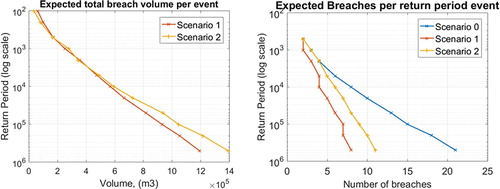
The expected number of breaches and total breach volumes in the entire system are given in Figure 6, for various return periods. An increase in expected breaches from scenario 1 to 2 is again observed, however, this difference is small in comparison to the expected breaches that would occur if system behaviour was not taken into account. Although most locations experience less breach volume in scenario 1 than in scenario 2, the higher number of breaches ensures that the expected overall breach volume is larger for extreme events.

Figure 6. Expected breaches and breach volumes per return period event in the system.

5. Conclusions

This study analyses the effect on flood hazard of two breaching triggering mechanisms in a system behaviour framework for the Dutch Rhine system. Variability in the load and strengths of the system are accounted for using 1D simulations in a Monte Carlo analysis. Potential breaches can occur dependent on water level in scenario 1 and both water level and duration in scenario 2, implemented using fragility curves and surfaces respectively. These fragility functions are adjusted to conform with the new protection standards in the Netherlands, and the results are compared in relation to hydraulic loads and breaching statistics.

As previously concluded by De Bruijn et al. (2016), it is clear that system behaviour has an impact on the downstream loads in the system, and as expected, this impact is generally reduced with the inclusion of duration in the failure mechanism. However, the results suggest that this reduction in impact is small for the modelled system, and even absent in terms of peak discharge, (Figure 7). As seen in the results, the changes in hydraulic loads will directly affect the probability of failure downstream, and the breach volume experienced when breached. The combination of these effects will have an overall effect on the hazard and thus risk in the system.

Figure 7. Return period discharges for Scenarios 0, 1 and 2, at locations P1_r, W6_l, L19_1 and I13_l. These locations can be seen on a map in Figure 2. Note that the x-axis scales are not the same per location Scenarios 0, 1 and 2 represent no system behaviour, system behaviour dependent on water level and system behaviour dependent on water level and duration, respectively.

The method and results presented have a number of limitations. Firstly, the effect of water level duration on the breach probability is very uncertain. The experts’ opinion on this effect differs significantly and the probabilities cannot be validated easily since there is a lack of data. Given that the events of interest are of extremely low probability, this drawback of validation is unlikely to be overcome. Secondly, the hydraulic loads inputs to the system have also been simplified by using generic wave-shapes. In reality, the floodwave may have much more variability, such as double peaks, as seen in the load data obtained from GRADE. Finally, the floodplains are represented by simple reservoirs here and do not represent the timing or volume of breach flow accurately. Besides, the water levels in the reservoirs are not directly related to local water depths which mean that this approach cannot be directly linked to flood impact models.

These simplifications mean that although this method is applicable to policy analyses on large scale (for systems understanding etc.), the method is not suitable for design purposes. The results can be considered representative of system behaviour and the effect of including water level duration in the dike breaching component.

An understanding of the likely behaviour in a system during extreme events has intrinsic value for flood risk strategy development, and may have applications in other fields such as emergency response and insurance. Other lowland river areas with a defence system in place, such as the Elbe, Danube, Po and the Vietnamese Red River could also benefit from such an analysis.

Recommendations for improving the method are to better represent the floodplains include the influence of the sea and the Meuse River on the area. Given the large uncertainties in system behaviour and the small effects observed when including duration of the water level, a more geotechnically accurate breaching mechanism to represent the influence of duration may not add value. However, a more structured expert opinion session may produce a better method of representing this uncertainty.

Finally, it should be noted that the results only count in case the system complies with the new safety standards, which is not the case at the moment. In fact, there are almost no embankments in the river that do comply currently. Assessing the system using an estimate of the current protection levels is likely to show a more pronounced effect of system behaviour in general, and may also change the effect of the duration dependency.

Acknowledgements

The authors would also like to thank the dike failure experts and other colleagues who contributed to the work.

Disclosure statement

No potential conflict of interest was reported by the author(s).

ORCID

A. Curran http://orcid.org/0000-0002-8643-1412

Additional information

Funding

This project has received funding from the European Union’s Horizon 2020 research and innovation programme under the Marie Skłodowska-Curie grant agreement No 676027.

Appendices

Appendix 1 – Failure probabilities, breach locations and trajects

The 62 breach locations used in the model are shown in Figure A1, and the associated trajectories and failure probabilities are shown in Table A1. The information from the breach locations is combined to generate the overall trajectory failure probabilities. The third column of the table shows the protection standard and the fourth and fifth columns show the calculated failure probabilities of these trajects in scenario 0, for both breach triggering mechanisms. As the fragility curves and surfaces were adjusted to meet the desired probabilities, these values should approximate the third column. The final two columns show the new failure probabilities when system behaviour is applied. In all cases, the failure probabilities decrease (return times increase) with respect to than their non-system behaviour equivalents.

Figure A1. Breach locations used in the model and associated dike sections.

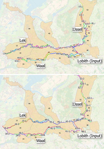
Table A1. Traject location failure probabilities are given in return period years. The protection standard is shown against the failure probabilities calculated with and without system behaviour for each dike breaching scenario. The values are rounded for clarity.

Trajectory Location	Associated Breach locations	Failure probability in return period years
		Protection Standard	Sc0 (Water level trigger)	Sc0 (Water level and duration trigger)	Sc1	Sc2
15_1	L16_r, L18_r, L20_r, L14_r, L21_r, L13_r	30,000	26,500	28,200	38,100	44,800
15_2	L23_r	30,000	23,200	50,100	23,200	56,500
16_1	W15_r, W17_r, W13_r, W14_r	30,000	30,900	50,500	368,000	437,000
16_2	L24_l	10,000	10,000	12,000	10,000	12,000
16_3	L19_l,	10,000	9880	8960	12,200	11,400
16_4	L15_l, L17_l, L12_l	10,000	11,200	9580	13,200	11,800
24_3	W12_l, W16_l	10,000	10,700	17,500	29,200	37,200
38_1	W11_l, W9_l	10,000	10,200	18,700	22,300	32,800
41_1	W5_l	10,000	7960	8290	8380	9030
41_2	W7_l, W6_l	3000	2460	2700	2550	2830
42_1	W1_l, W3_l	3000	3100	2970	3220	3080
43_1	L11_l, L10_l	10,000	9730	8430	12,700	10,600
43_2	L8_l, L7_l, L5_l	3000	2750	2490	2880	2640
43_3a	L4_l, L2_l, P2_l, W2_r	10,000	9810	9310	11,700	10,900
43_4a	W4_r	10,000	8280	8330	8680	9020
43_5	W10_r, W8_r	10,000	10,100	9140	12,800	11,400
44_1	L9_r	10,000	11,000	9390	12,900	11,100
45_1	L6_r	30,000	24,100	28,100	30,600	33,900
47_1	I2_l, I1_l, L1_r, L3_r	30,000	26,500	28,200	38,100	44,800
48_1	P3_r, P1_r, R2_r, R1_r	30,000	23,200	50,100	23,200	56,500
48_2	I3_r	30,000	30,900	50,500	368,000	437,000
49_2	I4_r	10,000	10,000	12,000	10,000	12,000
50_1	I6_r	10,000	9880	8960	12,200	11,400
51_1	I8_r, I7_r	10,000	11,200	9580	13,200	11,800
52_1	I15_l	10,000	10,700	17,500	29,200	37,200
52_2	I12_l, I9_l, I10_l, I11_l	10,000	10,200	18,700	22,300	32,800
52_3	I5_l	10,000	7960	8290	8380	9030
53_1	I13_r	3000	2460	2700	2550	2830
53_2	I14_r, I16_r	3000	3100	2970	3220	3080

Appendix 2 – Verheij van der Knaap parameters

The breach growth formula is shown in (A.1). The parameters input prior to calculation are given in Table A2, H is the difference in water level, and t is the time in hours since the breach occurred.$B\left(t\right)=B_0+f_1\frac{g^{1/2}{H}^{1.5}}{u_c}\mathrm{l}\mathrm{o}\mathrm{g}\left(1+\frac{f_{2}g}{u_c}t\right)\left(\mathrm{A}.1\right)$

Table A2. Verheij van der Knaap parameters used in the breach growth formulation.

Parameter name	Description	Range	Default value	Unit
f1	Empirical factor for breach width	0.5–5	1.3	–
f2	Empirical factor for breach width	0.01–1	0.04	–
Uc	Critical flow velocity	0.1–10	0.2	m/s
B0	Initial breach width	–	20	m
g	Acceleration due to Gravity	–	9.81	m/s^2

Appendix 3 – original and adjusted fragility curves

Below are the calculated original fragility curves calculated, represented as mean and standard deviation for each mechanism. For the two scenarios, the standard deviations were maintained, and the mean values were adjusted at each location so that the dike as a whole conformed to the new protection standards. As the change in mean values was the same for each mechanism, it is represented as a single value on the columns on the left.

Fragility curves calculated from BOA data, and the adjustments required to the means to conform to the new protection standards, for each scenario. See Figure A1 for locations of breaches on a map.

Table A3. Parameters of the calculated curves for each location. The sigma values for Overtopping, Piping and Macrostability are given in the first 3 columns. The final column shows the difference between the mu values calculated for scenario 2.

Location	Sigma values for mechanisms (m)			Difference between Mu values; Sc2–Sc1
	Overtopping	Piping	Macro-stability
L9_r	0.16	0.8	1.03	–0.08
L16_r	0.12	3.5	1.21	–1.07
L18_r	0.08	1.12	1.29	–0.15
L23_r	0.12	1.46	1.39	–0.39
L20_r	0.16	1.25	1.29	–0.16
L14_r	0.16	0.99	1.25	–0.11
L21_r	0.07	1.61	1.33	–0.34
L13_r	0.13	0.87	0.97	–0.06
I14_r	0.14	1.48	0.85	–0.36
I16_r	0.1	1.48	0.75	–0.31
I13_r	0.2	0.95	0.72	–0.18
I15_l	0.12	0.68	0.71	–0.13
I12_l	0.1	0.78	0.8	–0.15
I9_l	0.12	0.72	0.85	–0.1
I5_l	0.17	0.65	0.7	–0.14
I8_r	0.17	0.58	0.67	–0.07
I7_r	0.16	0.51	0.68	–0.07
I6_r	0.22	0.62	0.38	–0.04
I4_r	0.13	1.75	0.35	–0.41
I3_r	0.2	0.88	0.84	–0.13
P3_r	0.09	1.08	0.73	–0.08
P1_r	0.18	1.33	0.86	–0.12
R2_r	0.5	1.02	0.73	–0.08
R1_r	0.25	1.28	0.75	–0.15
I2_l	0.13	1.38	1.05	–0.13
I1_l	0.09	1.61	1.24	–0.14
L1_r	0.23	1.29	1.12	–0.08
L3_r	0.17	1.14	1.17	–0.16
L11_l	0.12	1.1	0.49	–0.06
L10_l	0.23	0.55	0.43	–0.02
L8_l	0.17	0.55	1.16	–0.05
L7_l	0.19	0.82	1.33	–0.07
L5_l	0.13	0.59	1.19	–0.02
L4_l	0.12	0.74	0.7	–0.04
L2_l	0.15	0.72	0.79	–0.02
P2_l	0.1	1.01	0.61	–0.08
W10_r	0.15	0.73	0.97	0.01
W8_r	0.24	0.84	1.27	–0.02
W4_r	0.18	0.93	1.94	–0.02
W2_r	0.12	1.09	2.79	–0.04
W1_l	0.17	1.36	0.86	–0.12
W3_l	0.14	1.83	0.87	–0.26
W7_l	0.15	1.41	1.53	–0.19
W6_l	0.17	1	1.49	–0.08
W5_l	0.11	1.28	0.56	–0.12
W11_l	0.25	0.72	1.55	–0.3
W9_l	0.14	0.65	1.41	–0.25
L15_l	0.13	0.8	0.68	–0.06
L24_l	0.1	0.77	1.44	–0.54
W15_r	0.2	0.2	0.2	–0.11
L17_l	0.15	2.02	0.54	–0.31
L6_r	0.18	0.77	1.11	–0.05
W12_l	0.13	0.11	0.11	–0.09
W16_l	0.15	0.14	0.14	–0.21
W17_r	0.14	0.16	0.16	–0.02
W13_r	0.07	0.16	0.16	–0.05
L19_l	0.14	0.88	0.49	–0.04
L22_l	0.15	1.13	0.47	–0.14
L12_l	0.07	1.01	0.57	–0.07
W14_r	0.19	0.2	0.2	–0.03
I10_l	0.11	0.84	1.07	–0.12
I11_l	0.11	0.88	1.26	–0.13

References

- Apel, H., B. Merz, and A. H. Thieken. 2009. “Influence of Dike Breaches on Flood Frequency Estimation.” Computers and Geosciences 35 (5). Elsevier: 907–923. doi:10.1016/j.cageo.2007.11.003.
- Assteerawatt, A., D. Tsaknias, F. Azemar, S. Ghosh, and A. Hilberts. 2016. “Large-scale and High-resolution Flood Risk Model for Japan.” FLOODrisk 2016 - 3rd European Conference on Flood Risk Management 11009: 1–5. doi:10.1051/e3sconf/20160711009.
- Bachmann, D., N. P. Huber, G. Johann, and H. Schüttrumpf. 2013. “Fragility Curves in Operational Dike Reliability Assessment.” Georisk: Assessment and Management of Risk for Engineered Systems and Geohazards 7 (1): 49–60. doi:10.1080/17499518.2013.767664.
- Courage, W., T. Vrouwenvelder, T. van Mierlo, and T. Schweckendiek. 2013. “System Behaviour in Flood Risk Calculations.” Georisk: Assessment and Management of Risk for Engineered Systems and Geohazards 7 (2): 62–76. doi:10.1080/17499518.2013.790732.
- De Bruijn, K. M., F. L. M. Diermanse, and J. V. L. Beckers. 2014. “An Advanced Method for Flood Risk Analysis in River Deltas, Applied to Societal Flood Fatality Risk in the Netherlands.” Natural Hazards and Earth System Sciences 14 (10): 2767–2781. doi:10.5194/nhess-14-2767-2014.
- De Bruijn, K. M., F. L. M. Diermanse, M. Van Der Doef, and F. Klijn. 2016. “Hydrodynamic System Behaviour : Its Analysis and Implications for Flood Risk Management.” FLOODrisk 2016 - 3rd European Conference on Flood Risk Management 11001. doi:10.1051/e3sconf/20160711001.
- Diermanse, F. L. M., K. M. De Bruijn, J. V. L. Beckers, and N. L. Kramer. 2014. “Importance Sampling for Efficient Modelling of Hydraulic Loads in the Rhine-Meuse Delta.” Stochastic Environmental Research and Risk Assessment 29 (3): 637–652. doi:10.1007/s00477-014-0921-4.
- Dunn, Christopher, P. Baker, and M. Fleming. 2016. “Flood Risk Management with HEC-WAT and the FRA Compute Option.” FLOODrisk 2016 - 3rd European Conference on Flood Risk Management 11006. doi:10.1051/e3sconf/20160711006.
- Dupuits, E. J. C., K. M. De Bruijn, F. L. M. Diermanse, and M. Kok. 2016. “Economically Optimal Safety Targets for Riverine Flood Defence Systems.” FLOODrisk 2016 - 3rd European Conference on Flood Risk Management 20004. doi:10.1051/e3sconf/20160720004.
- Falter, D., N. V. Dung, S. Vorogushyn, K. Schröter, Y. Hundecha, H. Kreibich, H. Apel, F. Theisselmann, and B. Merz. 2016. “Continuous, Large-scale Simulation Model for Flood Risk Assessments: Proof-of-Concept.” Journal of Flood Risk Management 9 (1): 3–21. doi:10.1111/jfr3.12105.
- Hegnauer, M., J. J. Beersma, H. F. P. van den Boogaard, T. A. Buishand, and R. H. Passchier. 2014. “Generator of Rainfall and Discharge Extremes (GRADE) for the Rhine and Meuse Basins. Final Report of GRADE 2.0,” 84.
- Jongejan, R. B., H. Stefess, N. Roode, W. Horst, and B. Maaskant. 2011. “The vnk2 Project: A Detailed, Large-scale Quantitative Flood Risk Analysis for the Netherlands.” International Conference on Flood Management 5, Proceedings 1: 301.
- Kiss, Tímea, I. Fehérváry, and K. Fiala. 2015. “Modelling the Hydrological Effects of a Levee Failure on the Lower Tisza River.” Journal of Environmental Geography 8 (1–2): 31–38. doi:10.1515/jengeo-2015-0004.
- Klerk, Wouter Jan. 2013. “Load Interdependencies of Flood Defences.” TU Delft, MSc Thesis, Delft University of Technology.
- Kok, M., R. Jongejan, M. Nieuwjaar, and I. Tanczos. 2017. “Fundamentals of Flood Protection.” Ministry of Infrastructure and the Environment and the Expertise Network for Flood Protection https://www.hkv.nl/upload/publication/Fundamentals_of_Flood_Protections_MK_WEBSITE.pdf.
- Levelt, O., S. van Vuren, J. Pol, r. van der Meij, D. Nugroho, W. ter Horst, R. Koopmans, P. van der Scheer, and A. de Kruif. 2017. “Uitwerking Methode Voor Bepaling Kostenreductie Rivierverruiming.” [In English: Elaboration Method for Determination Cost reduction River widening] 2016.
- Sellmeijer, Hans, J. L. de la Cruz, V. M. van Beek, and H. Knoeff. 2011. “Fine-tuning of the Backward Erosion Piping Model Through Small-scale, Medium-scale and IJkdijk Experiments.” European Journal of Environmental and Civil Engineering 15 (8): 1139–1154. doi:10.1080/19648189.2011.9714845.
- Slomp, Robert. 2016. Implementing Risk Based Flood Defence Standards. Amsterdam, Netherlands: Ministerie van Infrastructuur en Milieu.
- Steenbergen, H. M. G. M., B. L. Lassing, A. C. W. M. Vrouwenvelder, and P. H. Waarts. 2004. “Reliability Analysis of Flood Defence Systems.” Heron 49 (1): 51–73.
- Van, A. M., A. R. Koelewijn, and F. B. J. Barends. 2005. “Uplift Phenomenon: Model, Validation, and Design.” International Journal of Geomechanics 5 (2): 98–106. doi:10.1061/(ASCE)1532-3641(2005)5:2(98).
- van Mierlo, M. C. L. M., A. C. W. M. Vrouwenvelder, E. O. F. Calle, J. K. Vrijling, S. N. Jonkman, K. M. de Bruijn, and A. H. Weerts. 2003. “Effects of River System Behaviour on Flood Risk (Delft: Delft Cluster)”.
- van Mierlo, M. C. L. M., A. C. W. M. Vrouwenvelder, E. O. F. Calle, J. K. Vrijling, S. N. Jonkman, K. M. de Bruijn, and A. H. Weerts. 2007. “Assessment of Flood Risk Accounting for River System Behaviour.” International Journal of River Basin Management 5 (2): 93–104. doi:10.1080/15715124.2007.9635309.
- Verheij, H. J., and F. C. M. van der Knaap. 2002. “Modification Breach Growth Model in HIS-OM.” WL Delft Hydraulics Q 1: 1.
- Vorogushyn, S., P. D. Bates, K. de Bruijn, A. Castellarin, H. Kreibich, S. Priest, and B. Merz. 2017. “Evolutionary Leap in Large-scale Flood Risk Assessment Needed.” Wiley Interdisciplinary Reviews: Water (October): e1266. doi: 10.1002/wat2.1266
- Vorogushyn, S., B. Merz, and H. Apel. 2009. “Development of Dike Fragility Curves for Piping and Micro-instability Breach Mechanisms.” Natural Hazards and Earth System Science 9 (4): 1383–1401. doi:10.5194/nhess-9-1383-2009.
- Vorogushyn, S., B. Merz, K. E. Lindenschmidt, and H. Apel. 2010. “A New Methodology for Flood Hazard Assessment Considering Dike Breaches.” Water Resources Research 46 (8): 1–17. doi:10.1029/2009WR008475.
- Vrijling, J. K. 2001. “Probabilistic Design of Water Defense Systems in The Netherlands.” Reliability Engineering & System Safety 74 (3): 337–344. doi:10.1016/S0951-8320(01)00082-5.
- Vrouwenvelder, A. C. W. M., M. C. L. M. van Mierlo, E. O. F. Calle, A. A. Markus, T. Schweckendiek, and W. M. G. Courage. 2010. “Risk Analysis for Flood Protection Systems.” Main report, TNO and Deltares, Delft, the Netherlands.