Application of physics-informed neural networks to inverse problems in unsaturated groundwater flow

ABSTRACT

This paper investigates the application of Physics-Informed Neural Networks (PINNs) to inverse problems in unsaturated groundwater flow. PINNs are applied to the types of unsaturated groundwater flow problems modelled with the Richards partial differential equation and the van Genuchten constitutive model. The inverse problem is formulated here as a problem with known or measured values of the solution to the Richards equation at several spatio-temporal instances, and unknown values of solution at the rest of the problem domain and unknown parameters of the van Genuchten model. PINNs solve inverse problems by reformulating the loss function of a deep neural network such that it simultaneously aims to satisfy the measured values and the unknown values at a set of collocation points distributed across the problem domain. The novelty of the paper originates from the development of PINN formulations for the Richards equation that requires training of a single neural network. The results demonstrate that PINNs are capable of efficiently solving the inverse problem with relatively accurate approximation of the solution to the Richards equation and estimates of the van Genuchten model parameters.

KEYWORDS:

• Physics-informed
• neural
• network
• Richards
• unsaturated
• inverse
• infiltration
• groundwater

1. Introduction

Predictions of various problems in unsaturated soil mechanics, such as rainfall-induced landslides and excavation collapses, rely on thorough understanding and the capacity to model coupled hydro-mechanical process in soils (e.g. Zhang et al., 2018). Increasing the capacity for understanding and modelling hydromechanical processes in unsaturated soil mechanics contributes to developing strategies for mitigating potentially negative consequences of such events (e.g. Depina, Oguz, and Thakur, 2020). This study examines the capacity of Physics-Informed Neural Networks (PINNs) in solving unsaturated groundwater flow problems modelled by the Richards Partial Differential Equation (PDE) (Richards, 1931).

The Richards equation is a non-linear PDE and has been a great matter of interest in a wide range of fields including, among others, soil mechanics, agriculture, hydrogeology and reservoir engineering. The nonlinear nature of this equation is a reflection of the nonlinear relationship between the soil volumetric water content, θ, and the pressure head, ψ, which together with hydraulic conductivity, k form three primary variables of Richards equation. The primary variables are mutually dependent with θ and k often being expressed as a function of ψ, respectively, with the Water Retention Curve (WRC) and Hydraulic Conductivity Function (HCF). Both of these hydraulic functions are also known as constitutive relationships and are utilised to describe the characteristics of water and solute movement in soils (e.g. Schindler and Müller, 2017). Among several parametric models that are frequently used to represent these constitutive relationships (e.g. Abkenar, Rasoulzadeh, and Asghari, 2019), this study employs one of the most commonly used constitutive models, known as the van Genuchten model (Van Genuchten, 1980).

Solutions to the Richards equation with the van Genuchten model are commonly found by employing finite difference and finite element methods (e.g. Šimunek, Van Genuchten, and Šejna, 2012). An alternative approach is investigated in this study by finding solutions to the Richards equation with PINNs (e.g. Raissi, Perdikaris, and Karniadakis, 2019). The capacity of PINNs to solve partial and ordinary differential equations stems from the capabilities of Deep Neural Networks (DNNs) to server as a universal function approximator (Chen et al., 2020). PINNs extend the capacity of existing DNNs to solve PDEs by restricting the range of acceptable solutions through modifications of the loss function to the ones that enforce the PDE that governs the actual physics of the problem. In this way, this method extends the existing capacity of DNNs to approximate the solution of PDEs. It is achieved with a relatively simple feed-forward neural network architectures that utilise Automatic Differentiation (AD) techniques to efficiently evaluate the partial derivatives in the PDE to ensure that the PINN prediction satisfies the PDE across the problem domain. PINNs are investigated here due to their computational efficiency that can be advantageous in computationally demanding task in unsaturated soil mechanics involving parametric analysis, uncertainty quantification, real-time monitoring and inverse analysis.

This study builds on several earlier studies that investigated the application of PINNs to the Richards equation in Tartakovsky et al. (2018) and Bandai and Ghezzehei (2020). Bandai and Ghezzehei (2020) introduced a new framework for the inverse solution of the Richards equation to estimate WRC and HCF without introducing a specific constitutive model. This involved training three neural networks with the one approximating the solution, the Richards PDE in terms of θ, and the remaining two describing, respectively, WRC and HCF. Tartakovsky et al. (2018) employed PINNs to determine HCF of an unsaturated homogenous soil from synthetic matric potential data based on the two-dimensional time-dependent Richards equation. This study complements and extends the previous studies by investigating an inverse solution to the one-dimensional Richards PDE with the van Genuchten model. The adoption of the van Genuchten constitutive model allows the solution to the inverse problem to be found by training a single neural network. Additionally, inverse solutions to both the volumetric water content and the pressure head formulations of the Richards PDE were investigated to accommodate the respective measurements. The inverse problem is formulated in this study as a problem with known values of θ or ψ at several spatio-temporal instances, and unknown values of the Richards PDE variables at the rest of the problem domain and unknown parameters of the van Genuchten model. The performance of the PINN formulations on the inverse problem was examined on several examples with synthetically generated data and measurements from a water infiltration column test.

2. Physics-informed neural network (PINN)

2.1. Formulation

Mathematically, a deep network can be considered as a particular choice of a compositional function (Lu et al., 2019). This study employs a Feed forward Neural Network (FNN), also known as Multi-Layer Perceptron (MLP), which is constructed by applying linear and nonlinear transformations to the inputs recursively.

Let ${\mathcal{N}}^L(\mathit{x}):{\mathbb{R}}^{d_{in}}\to {\mathbb{R}}^{d_{out}}$ be an L-layer neural network, or a $(L-1)$-hidden layer neural network, with $N_l$ neurons in the lth layer $(N_0=d_{in},N_L=d_{out})$. Each layer is associated with a weight matrix, ${\mathit{W}}^l\in {\mathbb{R}}^{N_l\times N_{l-1}}$, and a bias vector, ${\mathit{b}}^l\in {\mathbb{R}}^{N_l}$. With a nonlinear activation function that is applied element-wise, σ, the FNN is recursively defined as follows (Lu et al., 2019): $\begin{array}{ccc}\mathrm{input}\mathrm{layer}:& {\mathcal{N}}^0(\mathit{x})=\mathit{x}\in {\mathbb{R}}^{d_{in}}& \\ \mathrm{hidden}\mathrm{layers}:& {\mathcal{N}}^l(\mathit{x})=\sigma ({\mathit{W}}^l{\mathcal{N}}^{l-1}+{\mathit{b}}^l)\in {\mathbb{R}}^{N_l},\\ & \mathrm{for}1\le l\le L-1\\ \\ \mathrm{output}\mathrm{layer}:& {\mathcal{N}}^L(\mathit{x})={\mathit{W}}^L{\mathcal{N}}^{L-1}+{\mathit{b}}^L\in {\mathbb{R}}^{d_{out}}& \end{array}$The activation function, σ, is commonly specified as the logistic sigmoid $\sigma (x)=1/(1-\exp (-x))$, hyperbolic tangent, $\sigma (x)=\tanh (x)$, or the rectified linear unit, $\sigma (x)=max(x,0)$.

One of the central properties of neural networks that will be used in the development of PINNs is the Automatic Differentiation (AD). AD is used to evaluate the derivatives of the network outputs with respect to the network inputs through the process of backpropagation (Rumelhart, Hinton, and Williams, 1986). The backpropagation process utilises the compositional structure of neural networks to apply the chain derivative rule repeatedly and compute the derivatives. The AD starts with a forward pass to compute the values of all of the variables, which is followed by a backward pass to compute the derivatives. Computing nth-order derivatives requires AD to be applied recursively n times. Additionally, it is important to note that the AD is applied on the neural network and not the data, thus allowing for the possibility to work with noisy data (e.g. Lu et al., 2019).

Given the introduction to neural networks and AD, the following section will introduce PINNs. Consider the following PDE, parameterised by $\mathit{\lambda }$, for the solution $u(\mathit{x})$ with $\mathit{x}=(x_1,\dots ,x_d)$ defined on a domain $\mathrm{\Omega }\subset {\mathbb{R}}^d$: (1) $f(\mathit{x}:\frac{\mathrm{\partial }u}{\mathrm{\partial }{x}_1},\dots \frac{\mathrm{\partial }u}{\mathrm{\partial }{x}_d}\frac{{\mathrm{\partial }}^{2}u}{\mathrm{\partial }{x}_1\mathrm{\partial }{x}_1},\frac{{\mathrm{\partial }}^{2}u}{\mathrm{\partial }{x}_1\mathrm{\partial }{x}_2}\dots \frac{{\mathrm{\partial }}^{2}u}{\mathrm{\partial }{x}_d\mathrm{\partial }{x}_d}\dots \mathit{\lambda })=0,\mathit{x}\in \mathrm{\Omega }$(1) with Dirichlet, Neumann, Robin or periodic Boundary Conditions (BC) represented by $\mathcal{B}(u,\mathit{x})=0\mathrm{on}\mathrm{\partial }\mathrm{\Omega }$Time-dependent problems are implemented such that t is considered as a component of $\mathit{x}$ with Ω containing the temporal domain. The Initial Conditions (IC) are treated as Dirichlet boundary conditions on the spatio-temporal domain.

The implementation of PINNs is illustrated in Figure 1 with mixed boundary conditions $u(\mathit{x})=g_D(\mathit{x})$ on ${\mathrm{\Gamma }}_D\subset \mathrm{\partial }\mathrm{\Omega }$ and $\frac{\mathrm{\partial }u}{\mathrm{\partial }\mathit{n}}=g_R(u,\mathit{x})$ on ${\mathrm{\Gamma }}_R\subset \mathrm{\partial }\mathrm{\Omega }$.

Figure 1. PINN illustration adapted from Lu et al. (2019).

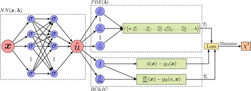
The implementation of a PINN starts by constructing a neural network $\hat{u}(\mathit{x}\mathit{\chi })$ as an approximate solution of $u(\mathit{x})$. The input to the neural network is $\mathit{x}$ and the output is vector of the same dimension as u. Weight matrices and bias vectors of the neural network $\hat{u}$ are denoted with $\mathit{\chi }=\{{\mathit{W}}^l,{\mathit{b}}^l{\}}_{1\le l\le L}$.

Following the specification of the neural network, it is necessary to ensure that the neural network satisfies the physics defined by the PDE and the boundary conditions. This is usually implemented by restricting $\hat{u}$ on a set of collocation points $\mathcal{T}=\{{\mathit{x}}_1,{\mathit{x}}_1,\dots ,{\mathit{x}}_{|\mathcal{T}|},\}$ of size $|\mathcal{T}|$. Generally, $\mathcal{T}$ can be composed of collocation points in the domain ${\mathcal{T}}_f\subset \mathrm{\Omega }$ and on the boundary ${\mathcal{T}}_b\subset \mathrm{\partial }\mathrm{\Omega }$. The discrepancy between the neural network $\hat{u}$ and the physical constraints is measured through the loss function, defined as weighted sum of the $L^2$ norm of the residuals for the collocation points in the domain and on the boundary: (2) $\mathcal{L}\left(\mathit{\chi }\mathcal{T}\right)=w_f{\mathcal{L}}_f\left(\mathit{\chi }{\mathcal{T}}_f\right)+w_b{\mathcal{L}}_b\left(\mathit{\chi }{\mathcal{T}}_b\right)$(2) where $w_f$ and $w_b$ are the weights, and (3) $\begin{array}{rl}& {\mathcal{L}}_f(\mathit{\chi }{\mathcal{T}}_f)=\frac{1}{|{\mathcal{T}}_f|}\\ & \sum _{\mathit{x}\in {\mathcal{T}}_f}^{}{\Vert f(\mathit{x}:\frac{\mathrm{\partial }\hat{u}}{\mathrm{\partial }{x}_1},\dots \frac{\mathrm{\partial }\hat{u}}{\mathrm{\partial }{x}_d}\frac{{\mathrm{\partial }}^2\hat{u}}{\mathrm{\partial }{x}_1\mathrm{\partial }{x}_1},\frac{{\mathrm{\partial }}^2\hat{u}}{\mathrm{\partial }{x}_1\mathrm{\partial }{x}_2}\dots \frac{{\mathrm{\partial }}^2\hat{u}}{\mathrm{\partial }{x}_d\mathrm{\partial }{x}_d}\dots \mathit{\lambda })\Vert }_2^2\end{array}$(3) (4) ${\mathcal{L}}_b(\mathit{\chi }{\mathcal{T}}_b)=\frac{1}{|{\mathcal{T}}_b|}\sum _{\mathit{x}\in {\mathcal{T}}_b}^{}{\Vert \mathcal{B}(\hat{u},\mathit{x})\Vert }_2^2$(4) The derivatives in the loss function are calculated with AD, which is available in machine learning libraries such as TensorFlow (Abadi et al., 2015) and PyTorch (Paszke et al., 2019).

The final step in the implementation of PINNs is the training stage in which the set of parameters in $\mathit{\chi }$ is varied to minimise the loss function $\mathcal{L}(\mathit{\chi }\mathcal{T})$. The loss function is usually highly nonlinear and non-convex with respect to $\mathit{\chi }$ and the optimisation is commonly performed with gradient-based optimisers.

2.2. Inverse problem

In addition to the forward problem, PINNs can be easily applied to inverse problems with unknown parameters $\mathit{\lambda }$ in Equation (1(1) $f(\mathit{x}:\frac{\mathrm{\partial }u}{\mathrm{\partial }{x}_1},\dots \frac{\mathrm{\partial }u}{\mathrm{\partial }{x}_d}\frac{{\mathrm{\partial }}^{2}u}{\mathrm{\partial }{x}_1\mathrm{\partial }{x}_1},\frac{{\mathrm{\partial }}^{2}u}{\mathrm{\partial }{x}_1\mathrm{\partial }{x}_2}\dots \frac{{\mathrm{\partial }}^{2}u}{\mathrm{\partial }{x}_d\mathrm{\partial }{x}_d}\dots \mathit{\lambda })=0,\mathit{x}\in \mathrm{\Omega }$(1) ). In the case of an inverse problem, it is considered that there are some additional information on points ${\mathcal{T}}_i\subset \mathrm{\Omega }$ in addition to the earlier training points in the domain and on the boundary conditions: (5) $\mathcal{I}(u,\mathit{x})=0\mathrm{for}\mathit{x}\in {\mathcal{T}}_i$(5) The implementation of the inverse problem is often relatively straightforward, with the only difference with respect to the forward problem being the loss function with an additional term: (6) $\mathcal{L}(\mathit{\chi },\mathit{\lambda }\mathcal{T})=w_f{\mathcal{L}}_f(\mathit{\chi },\mathit{\lambda }{\mathcal{T}}_f)+w_b{\mathcal{L}}_b(\mathit{\chi },\mathit{\lambda }{\mathcal{T}}_b)+w_i{\mathcal{L}}_i(\mathit{\chi },\mathit{\lambda }{\mathcal{T}}_i)$(6) where $w_i$ is the weight and (7) ${\mathcal{L}}_i(\mathit{\chi },\mathit{\lambda }{\mathcal{T}}_i)=\frac{1}{|{\mathcal{T}}_i|}\sum _{\mathit{x}\in {\mathcal{T}}_i}^{}{\Vert \mathcal{I}(\hat{u},\mathit{x})\Vert }_2^2$(7) The training stage is then done by optimising $\mathit{\chi }$ and $\mathit{\lambda }$ simultaneously: (8) ${\mathit{\chi }}^{\ast },\hat{\mathit{\lambda }}=\arg \underset{\mathit{\chi },\mathit{\lambda }}{min}\mathcal{L}(\mathit{\chi },\mathit{\lambda }\mathcal{T})$(8) where ${\mathit{\chi }}^{\ast }$ and $\hat{\mathit{\lambda }}$ are, respectively, optima of $\mathit{\chi }$ and $\mathit{\lambda }$. Finding a solution to the inverse problem based on Equation (8(8) ${\mathit{\chi }}^{\ast },\hat{\mathit{\lambda }}=\arg \underset{\mathit{\chi },\mathit{\lambda }}{min}\mathcal{L}(\mathit{\chi },\mathit{\lambda }\mathcal{T})$(8) ) is relatively straightforward and computationally efficient, especially in the case of linear PDEs. However, it was found in some nonlinear problems that the optimisation process is dominated by gradients with respect to $\mathit{\chi }$, which results in the optimisation process not advancing toward a more optimal $\mathit{\lambda }$ value or that the optimal solution results in physically inconsistent values (e.g. negative values of positive constants). Although it is likely that these issues can be addressed by reformulating the loss function and introducing constraints to the optimisation formulation in Equation (8(8) ${\mathit{\chi }}^{\ast },\hat{\mathit{\lambda }}=\arg \underset{\mathit{\chi },\mathit{\lambda }}{min}\mathcal{L}(\mathit{\chi },\mathit{\lambda }\mathcal{T})$(8) ), this study aims to resolve them by reformulating the inverse problem in Equation (8(8) ${\mathit{\chi }}^{\ast },\hat{\mathit{\lambda }}=\arg \underset{\mathit{\chi },\mathit{\lambda }}{min}\mathcal{L}(\mathit{\chi },\mathit{\lambda }\mathcal{T})$(8) ) into a double-loop formulation: (9a) $\hat{\mathit{\lambda }}=\arg \underset{\mathit{\lambda }}{min}\left[\underset{\mathit{\chi }}{min}\mathcal{L}(\mathit{\chi },\mathit{\lambda }\mathcal{T})\right]$(9a) (9b) $\mathrm{subjected}\mathrm{to}:g_k(\mathit{\lambda })\le 0k=1,\dots ,N_g$(9b) (9c) ${\mathit{\lambda }}_l\le \mathit{\lambda }\le {\mathit{\lambda }}_u$(9c) where $\hat{\mathit{\lambda }}$ is an optimum, $g_{k}k=1,\dots ,N_g$ are constraint functions, and ${\mathit{\lambda }}_l$ and ${\mathit{\lambda }}_u$ are the lower and upper bounds, respectively. The outer loop of the algorithm will be optimising $\mathit{\lambda }$ values and enforcing constraints on the $\mathit{\lambda }$ values. The outer loop will be implemented with the global optimisation Cross Entropy (CE) algorithm (Botev et al., 2013), while the inner loop will utilise the gradient-based algorithms commonly available in machine learning libraries. The CE algorithm was selected due to its robust performance as a global optimisation algorithm and the relatively straightforward implementation (e.g. Botev et al., 2013). It is expected that similar performance can be achieved with alternative global optimisation algorithms (e.g. Genetic algorithm).

Research on the generalisation error for the application of PINNs to inverse problems is ongoing and more information can be found for example in Raissi, Perdikaris, and Karniadakis (2019) and Mishra and Molinaro (2021).

3. PINN for the Richards equation

3.1. Richards equation

The Richards equation is a nonlinear PDE that captures the flow of water in unsaturated zone (Richards, 1931). One-dimensional form of the Richards equation is given by (10) $\frac{\mathrm{\partial }\theta }{\mathrm{\partial }t}=\frac{\mathrm{\partial }}{\mathrm{\partial }x}\left[k\frac{\mathrm{\partial }\psi }{\mathrm{\partial }x}\right]+\frac{\mathrm{\partial }k}{\mathrm{\partial }x}$(10) where θ is the volumetric soil water content($L^3\cdot L^{-3}$), t is the time (T), x is the vertical dimension (L), k is the hydraulic conductivity ($L\cdot T^{-1}$) and ψ is the pressure head (L). The WRC and HCF relationships can be specified by the van Genuchten model (Van Genuchten, 1980): (11a) $k=k_s{\mathrm{\Theta }}^{1/2}{[1-{(1-{\mathrm{\Theta }}^{1/m})}^m]}^2$(11a) (11b) $\mathrm{\Theta }=\{\begin{array}{cc}{(1+|\alpha \psi {|}^n)}^{-m}& \psi <0\\ 1& \psi \ge 0\end{array}$(11b) (11c) $\mathrm{\Theta }=\frac{\theta -{\theta }_r}{{\theta }_s-{\theta }_r}$(11c) where $k_s$ is the saturated hydraulic conductivity, Θ is the relative saturation, ${\theta }_s$ and ${\theta }_r$ are, respectively, the saturated and residual volumetric water contents, α ($L^{-1}$), n, and m are the model parameters, where $m=1-1/n$. Equation (11a(11a) $k=k_s{\mathrm{\Theta }}^{1/2}{[1-{(1-{\mathrm{\Theta }}^{1/m})}^m]}^2$(11a) ) specifies the HCF and Equation (11b(11b) $\mathrm{\Theta }=\{\begin{array}{cc}{(1+|\alpha \psi {|}^n)}^{-m}& \psi <0\\ 1& \psi \ge 0\end{array}$(11b) ) the WRC relationship.

3.2. Pressure head formulation

Equation (10(10) $\frac{\mathrm{\partial }\theta }{\mathrm{\partial }t}=\frac{\mathrm{\partial }}{\mathrm{\partial }x}\left[k\frac{\mathrm{\partial }\psi }{\mathrm{\partial }x}\right]+\frac{\mathrm{\partial }k}{\mathrm{\partial }x}$(10) ) is reformulated to implement the PINN methodology for the Richards equation in terms of the pressure head, ψ as follows: (12) $\frac{\mathrm{\partial }\theta }{\mathrm{\partial }t}=\frac{\mathrm{\partial }k}{\mathrm{\partial }x}\frac{\mathrm{\partial }\psi }{\mathrm{\partial }x}+k\frac{\mathrm{\partial }{\psi }^2}{\mathrm{\partial }{x}^2}+\frac{\mathrm{\partial }k}{\mathrm{\partial }x}$(12) The equation is then reformulated to express the partial derivates of θ and k with respect to ψ. (13) $\frac{\mathrm{\partial }\theta }{\mathrm{\partial }\psi }\frac{\mathrm{\partial }\psi }{\mathrm{\partial }t}=\frac{\mathrm{\partial }k}{\mathrm{\partial }\psi }\frac{\mathrm{\partial }\psi }{\mathrm{\partial }x}\frac{\mathrm{\partial }\psi }{\mathrm{\partial }x}+k\frac{\mathrm{\partial }{\psi }^2}{\mathrm{\partial }{x}^2}+\frac{\mathrm{\partial }k}{\mathrm{\partial }\psi }\frac{\mathrm{\partial }\psi }{\mathrm{\partial }x}$(13) Finally, the following expression is obtained as (14) $C\frac{\mathrm{\partial }\psi }{\mathrm{\partial }t}=\frac{\mathrm{\partial }k}{\mathrm{\partial }\psi }{\left(\frac{\mathrm{\partial }\psi }{\mathrm{\partial }x}\right)}^2+k\frac{\mathrm{\partial }{\psi }^2}{\mathrm{\partial }{x}^2}+\frac{\mathrm{\partial }k}{\mathrm{\partial }\psi }\frac{\mathrm{\partial }\psi }{\mathrm{\partial }x}$(14) where $C=\mathrm{\partial }\theta /\mathrm{\partial }\psi$ is known as the water storage function. The water storage function is evaluated analytically based on the adopted van Genuchten model as follows: (15) $C=\frac{\mathrm{\partial }\theta }{\mathrm{\partial }\psi }=\frac{\mathrm{\partial }\theta }{\mathrm{\partial }\mathrm{\Theta }}\frac{\mathrm{\partial }\mathrm{\Theta }}{\mathrm{\partial }\psi }=({\theta }_s-{\theta }_r)\frac{\mathrm{\partial }\mathrm{\Theta }}{\mathrm{\partial }\psi }$(15) where $\mathrm{\partial }\mathrm{\Theta }/\mathrm{\partial }\psi$ is calculated based on the factorisation of the Richards equation as shown in Rai and Tripathi (2019): (16) $\frac{\mathrm{\partial }\mathrm{\Theta }}{\mathrm{\partial }\psi }=-\frac{\alpha m\mathrm{sign}(\psi )}{1-m}{\mathrm{\Theta }}^{(1+m)/m}{\{{\mathrm{\Theta }}^{-1/m}-1\}}^m$(16) The partial derivative $\mathrm{\partial }k/\mathrm{\partial }\psi$ is calculated analytically based on the van Genuchten model: (17) $\frac{\mathrm{\partial }k}{\mathrm{\partial }\psi }=\frac{\mathrm{\partial }k}{\mathrm{\partial }\mathrm{\Theta }}\frac{\mathrm{\partial }\mathrm{\Theta }}{\mathrm{\partial }\theta }\frac{\mathrm{\partial }\theta }{\mathrm{\partial }\psi }=\frac{C}{{\theta }_s-{\theta }_r}\frac{\mathrm{\partial }k}{\mathrm{\partial }\mathrm{\Theta }}=\frac{\mathrm{\partial }\mathrm{\Theta }}{\mathrm{\partial }\psi }\frac{\mathrm{\partial }k}{\mathrm{\partial }\mathrm{\Theta }}$(17) where $\mathrm{\partial }\mathrm{\Theta }/\mathrm{\partial }\theta =1/({\theta }_s-{\theta }_r)$. The partial derivative $\mathrm{\partial }k/\mathrm{\partial }\mathrm{\Theta }$ is determined from the van Genuchten model, as shown in Rai and Tripathi (2019): (18) $\begin{array}{rl}\frac{\mathrm{\partial }k}{\mathrm{\partial }\mathrm{\Theta }}& =2k_s{\mathrm{\Theta }}^{1/2}[1-{(1-{\mathrm{\Theta }}^{1/m})}^m]\left[{(1-{\mathrm{\Theta }}^{1/m})}^{m-1}\left({\mathrm{\Theta }}^{1/m-1}\right)\right]\\ & +\frac{k_s}{2}{\mathrm{\Theta }}^{-1/2}{[1-{(1-{\mathrm{\Theta }}^{1/m})}^m]}^2\end{array}$(18) In case of heterogeneous soils and known properties of spatially variable properties, the partial derivatives could be calculated by providing the known values of the material properties directly in the analytical expressions for the partial derivatives. In the case of an inverse problem, such as the ones studied here, additional studies are needed to investigate the potential of PINNs in solving inverse problems with spatially variable material properties.

To be consistent with the expression in Equation (1(1) $f(\mathit{x}:\frac{\mathrm{\partial }u}{\mathrm{\partial }{x}_1},\dots \frac{\mathrm{\partial }u}{\mathrm{\partial }{x}_d}\frac{{\mathrm{\partial }}^{2}u}{\mathrm{\partial }{x}_1\mathrm{\partial }{x}_1},\frac{{\mathrm{\partial }}^{2}u}{\mathrm{\partial }{x}_1\mathrm{\partial }{x}_2}\dots \frac{{\mathrm{\partial }}^{2}u}{\mathrm{\partial }{x}_d\mathrm{\partial }{x}_d}\dots \mathit{\lambda })=0,\mathit{x}\in \mathrm{\Omega }$(1) ), the pressure head PINN formulation for the Richards equation is defined as (19) $f(x,t:\frac{\mathrm{\partial }\psi }{\mathrm{\partial }x},\frac{\mathrm{\partial }\psi }{\mathrm{\partial }t}\frac{{\mathrm{\partial }}^2\psi }{\mathrm{\partial }{x}^2}\mathit{\lambda })=C\frac{\mathrm{\partial }\psi }{\mathrm{\partial }t}-\frac{\mathrm{\partial }k}{\mathrm{\partial }\psi }{\left(\frac{\mathrm{\partial }\psi }{\mathrm{\partial }x}\right)}^2-k\frac{\mathrm{\partial }{\psi }^2}{\mathrm{\partial }{x}^2}-\frac{\mathrm{\partial }k}{\mathrm{\partial }\psi }\frac{\mathrm{\partial }\psi }{\mathrm{\partial }x}=0$(19) where $\mathit{\lambda }=[k_s,{\theta }_s,{\theta }_r,\alpha ,n{]}^T$ is the vector that parameterises the Richards equation.

3.3. Volumetric water formulation

Equation (10(10) $\frac{\mathrm{\partial }\theta }{\mathrm{\partial }t}=\frac{\mathrm{\partial }}{\mathrm{\partial }x}\left[k\frac{\mathrm{\partial }\psi }{\mathrm{\partial }x}\right]+\frac{\mathrm{\partial }k}{\mathrm{\partial }x}$(10) ) is reformulated to implement the PINN methodology for the Richards equation in terms of the volumetric water content, θ, starting with the following expression: (20) $\frac{\mathrm{\partial }\theta }{\mathrm{\partial }t}=\frac{\mathrm{\partial }k}{\mathrm{\partial }x}\frac{\mathrm{\partial }\psi }{\mathrm{\partial }x}+k\frac{\mathrm{\partial }}{\mathrm{\partial }x}\left(\frac{\mathrm{\partial }\psi }{\mathrm{\partial }x}\right)+\frac{\mathrm{\partial }k}{\mathrm{\partial }x}$(20) The partial derivatives involving ψ are expressed in terms of θ by using the chain derivative rule: (21) $\frac{\mathrm{\partial }\theta }{\mathrm{\partial }t}=\frac{\mathrm{\partial }k}{\mathrm{\partial }x}\frac{\mathrm{\partial }\psi }{\mathrm{\partial }\theta }\frac{\mathrm{\partial }\theta }{\mathrm{\partial }x}+k\frac{\mathrm{\partial }}{\mathrm{\partial }x}\left(\frac{\mathrm{\partial }\psi }{\mathrm{\partial }\theta }\frac{\mathrm{\partial }\theta }{\mathrm{\partial }x}\right)+\frac{\mathrm{\partial }k}{\mathrm{\partial }x}$(21) The expression is further evaluated by rewriting the second term on the right side: (22) $\frac{\mathrm{\partial }\theta }{\mathrm{\partial }t}=\frac{\mathrm{\partial }k}{\mathrm{\partial }x}\frac{\mathrm{\partial }\psi }{\mathrm{\partial }\theta }\frac{\mathrm{\partial }\theta }{\mathrm{\partial }x}+k\frac{{\mathrm{\partial }}^2\psi }{\mathrm{\partial }x\mathrm{\partial }\theta }\frac{\mathrm{\partial }\theta }{\mathrm{\partial }x}+k\frac{\mathrm{\partial }\psi }{\mathrm{\partial }\theta }\frac{{\mathrm{\partial }}^2\theta }{\mathrm{\partial }{x}^2}+\frac{\mathrm{\partial }k}{\mathrm{\partial }x}$(22) The partial derivative $\mathrm{\partial }k/\mathrm{\partial }x$ was rewritten as follows: (23) $\frac{\mathrm{\partial }\theta }{\mathrm{\partial }t}=\frac{\mathrm{\partial }k}{\mathrm{\partial }\theta }\frac{\mathrm{\partial }\psi }{\mathrm{\partial }\theta }\frac{\mathrm{\partial }\theta }{\mathrm{\partial }x}\frac{\mathrm{\partial }\theta }{\mathrm{\partial }x}+k\frac{{\mathrm{\partial }}^2\psi }{\mathrm{\partial }x\mathrm{\partial }\theta }\frac{\mathrm{\partial }\theta }{\mathrm{\partial }x}+k\frac{\mathrm{\partial }\psi }{\mathrm{\partial }\theta }\frac{{\mathrm{\partial }}^2\theta }{\mathrm{\partial }{x}^2}+\frac{\mathrm{\partial }k}{\mathrm{\partial }\theta }\frac{\mathrm{\partial }\theta }{\mathrm{\partial }x}$(23) Finally, the expression was rewritten by introducing $1/C=\mathrm{\partial }\psi /\mathrm{\partial }\theta$: (24) $C\frac{\mathrm{\partial }\theta }{\mathrm{\partial }t}=\frac{\mathrm{\partial }k}{\mathrm{\partial }\theta }{\left(\frac{\mathrm{\partial }\theta }{\mathrm{\partial }x}\right)}^2+kC\frac{{\mathrm{\partial }}^2\psi }{\mathrm{\partial }x\mathrm{\partial }\theta }\frac{\mathrm{\partial }\theta }{\mathrm{\partial }x}+k\frac{{\mathrm{\partial }}^2\theta }{\mathrm{\partial }{x}^2}+C\frac{\mathrm{\partial }k}{\mathrm{\partial }\theta }\frac{\mathrm{\partial }\theta }{\mathrm{\partial }x}$(24) The second-order partial derivative in the second term on the right side of the expression is calculated as (25) $\frac{{\mathrm{\partial }}^2\psi }{\mathrm{\partial }x\mathrm{\partial }\theta }=\frac{\mathrm{\partial }}{\mathrm{\partial }x}\left(\frac{\mathrm{\partial }\psi }{\mathrm{\partial }\theta }\right)$(25) where $\mathrm{\partial }\psi /\mathrm{\partial }\theta$ is specified based on Equation (15(15) $C=\frac{\mathrm{\partial }\theta }{\mathrm{\partial }\psi }=\frac{\mathrm{\partial }\theta }{\mathrm{\partial }\mathrm{\Theta }}\frac{\mathrm{\partial }\mathrm{\Theta }}{\mathrm{\partial }\psi }=({\theta }_s-{\theta }_r)\frac{\mathrm{\partial }\mathrm{\Theta }}{\mathrm{\partial }\psi }$(15) ): (26) $\frac{\mathrm{\partial }\psi }{\mathrm{\partial }\theta }=\frac{1}{C}=\frac{1}{{\theta }_s-{\theta }_r}{\left(\frac{\mathrm{\partial }\mathrm{\Theta }}{\mathrm{\partial }\psi }\right)}^{-1}=-\frac{1}{{\theta }_s-{\theta }_r}\frac{1-m}{\alpha m\mathrm{sign}(\psi )}{\mathrm{\Theta }}^{-(1+m)/m}{\{{\mathrm{\Theta }}^{-1/m}-1\}}^{-m}$(26) From the expression it can be observed that $\mathrm{\partial }\psi /\mathrm{\partial }\theta$ is expressed in terms of Θ with the $\mathrm{sign}(\psi )=1$ for unsaturated conditions, thus eliminating ψ from the expression. Taking the partial derivative of Equation (26(26) $\frac{\mathrm{\partial }\psi }{\mathrm{\partial }\theta }=\frac{1}{C}=\frac{1}{{\theta }_s-{\theta }_r}{\left(\frac{\mathrm{\partial }\mathrm{\Theta }}{\mathrm{\partial }\psi }\right)}^{-1}=-\frac{1}{{\theta }_s-{\theta }_r}\frac{1-m}{\alpha m\mathrm{sign}(\psi )}{\mathrm{\Theta }}^{-(1+m)/m}{\{{\mathrm{\Theta }}^{-1/m}-1\}}^{-m}$(26) ) with respect to x results with the following expression: (27) $\begin{array}{rl}\frac{\mathrm{\partial }}{\mathrm{\partial }x}\left(\frac{\mathrm{\partial }\psi }{\mathrm{\partial }\theta }\right)& =-\frac{1}{{\theta }_s-{\theta }_r}\frac{1-m}{\alpha m\mathrm{sign}(\psi )}\\ & [-\frac{1+m}{m}{\mathrm{\Theta }}^{(2m-1)/m}{\{{\mathrm{\Theta }}^{-1/m}-1\}}^m\frac{\mathrm{\partial }\mathrm{\Theta }}{\mathrm{\partial }x}\\ & +{\mathrm{\Theta }}^{-(2m+2)/m}{\{{\mathrm{\Theta }}^{-1/m}-1\}}^{m-1}\frac{\mathrm{\partial }\mathrm{\Theta }}{\mathrm{\partial }x}]\end{array}$(27) The partial derivative $\mathrm{\partial }\mathrm{\Theta }/\mathrm{\partial }x$ is expressed as $\mathrm{\partial }\theta /\mathrm{\partial }x$ by applying the chain rule as follows: (28) $\frac{\mathrm{\partial }\mathrm{\Theta }}{\mathrm{\partial }x}=\frac{\mathrm{\partial }\mathrm{\Theta }}{\mathrm{\partial }\theta }\frac{\mathrm{\partial }\theta }{\mathrm{\partial }x}=\frac{1}{{\theta }_s-{\theta }_r}\frac{\mathrm{\partial }\theta }{\mathrm{\partial }x}$(28) This expression is then integrated in Equation (27(27) $\begin{array}{rl}\frac{\mathrm{\partial }}{\mathrm{\partial }x}\left(\frac{\mathrm{\partial }\psi }{\mathrm{\partial }\theta }\right)& =-\frac{1}{{\theta }_s-{\theta }_r}\frac{1-m}{\alpha m\mathrm{sign}(\psi )}\\ & [-\frac{1+m}{m}{\mathrm{\Theta }}^{(2m-1)/m}{\{{\mathrm{\Theta }}^{-1/m}-1\}}^m\frac{\mathrm{\partial }\mathrm{\Theta }}{\mathrm{\partial }x}\\ & +{\mathrm{\Theta }}^{-(2m+2)/m}{\{{\mathrm{\Theta }}^{-1/m}-1\}}^{m-1}\frac{\mathrm{\partial }\mathrm{\Theta }}{\mathrm{\partial }x}]\end{array}$(27) ): (29) $\begin{array}{rl}\frac{\mathrm{\partial }}{\mathrm{\partial }x}\left(\frac{\mathrm{\partial }\psi }{\mathrm{\partial }\theta }\right)& =-\frac{1}{({\theta }_s-{\theta }_r{)}^2}\frac{1-m}{\alpha m\mathrm{sign}(\psi )}\frac{\mathrm{\partial }\theta }{\mathrm{\partial }x}\\ & [-\frac{1+m}{m}{\mathrm{\Theta }}^{(2m-1)/m}{\{{\mathrm{\Theta }}^{-1/m}-1\}}^m\\ & +{\mathrm{\Theta }}^{-(2m+2)/m}{\{{\mathrm{\Theta }}^{-1/m}-1\}}^{m-1}]\end{array}$(29) The partial derivative $\mathrm{\partial }k/\mathrm{\partial }\theta$ is evaluated analytically based on the van Genucthen model: (30) $\frac{\mathrm{\partial }k}{\mathrm{\partial }\theta }=\frac{\mathrm{\partial }k}{\mathrm{\partial }\mathrm{\Theta }}\frac{\mathrm{\partial }\mathrm{\Theta }}{\mathrm{\partial }\theta }=\frac{\mathrm{\partial }k}{\mathrm{\partial }\mathrm{\Theta }}\frac{1}{{\theta }_s-{\theta }_r}$(30) where $\mathrm{\partial }k/\mathrm{\partial }\mathrm{\Theta }$ is defined in Equation (18(18) $\begin{array}{rl}\frac{\mathrm{\partial }k}{\mathrm{\partial }\mathrm{\Theta }}& =2k_s{\mathrm{\Theta }}^{1/2}[1-{(1-{\mathrm{\Theta }}^{1/m})}^m]\left[{(1-{\mathrm{\Theta }}^{1/m})}^{m-1}\left({\mathrm{\Theta }}^{1/m-1}\right)\right]\\ & +\frac{k_s}{2}{\mathrm{\Theta }}^{-1/2}{[1-{(1-{\mathrm{\Theta }}^{1/m})}^m]}^2\end{array}$(18) ). To be consistent with the expression in Equation (1(1) $f(\mathit{x}:\frac{\mathrm{\partial }u}{\mathrm{\partial }{x}_1},\dots \frac{\mathrm{\partial }u}{\mathrm{\partial }{x}_d}\frac{{\mathrm{\partial }}^{2}u}{\mathrm{\partial }{x}_1\mathrm{\partial }{x}_1},\frac{{\mathrm{\partial }}^{2}u}{\mathrm{\partial }{x}_1\mathrm{\partial }{x}_2}\dots \frac{{\mathrm{\partial }}^{2}u}{\mathrm{\partial }{x}_d\mathrm{\partial }{x}_d}\dots \mathit{\lambda })=0,\mathit{x}\in \mathrm{\Omega }$(1) ), the VWC PINN formulation for the Richards equation is defined as (31) $f(x,t:\frac{\mathrm{\partial }\theta }{\mathrm{\partial }x},\frac{\mathrm{\partial }\theta }{\mathrm{\partial }t}\frac{{\mathrm{\partial }}^2\theta }{\mathrm{\partial }{x}^2}\mathit{\lambda })=C\frac{\mathrm{\partial }\theta }{\mathrm{\partial }t}-\frac{\mathrm{\partial }k}{\mathrm{\partial }\theta }{\left(\frac{\mathrm{\partial }\theta }{\mathrm{\partial }x}\right)}^2-kC\frac{{\mathrm{\partial }}^2\psi }{\mathrm{\partial }x\mathrm{\partial }\theta }\frac{\mathrm{\partial }\theta }{\mathrm{\partial }x}-k\frac{{\mathrm{\partial }}^2\theta }{\mathrm{\partial }{x}^2}-C\frac{\mathrm{\partial }k}{\mathrm{\partial }\theta }\frac{\mathrm{\partial }\theta }{\mathrm{\partial }x}=0$(31) where $\mathit{\lambda }=[k_s,{\theta }_s,{\theta }_r,\alpha ,n{]}^T$ is the vector that parameterises the Richards equation.

4. Inverse problem

4.1. Introduction

This section investigates the application of PINNs for Richards equation for the inverse problem with both the pressure head and VWC formulations. The dataset for the inverse problem was generated by using a finite-difference code from Ireson (2020) by solving the Richards equation in the domain $\mathrm{\Omega }=[x_0,x_1]\times [0,T]$ where $x_0=0$ m, $x_1=2$ m, and $T=259,200$  s. The initial conditions are defined as $\psi (x,0)=-x$ with the boundary conditions being specified with a fixed pressure head on the top $\psi (x_1,t)=0.1$ m and impervious boundary at the base of the model, specified by $\mathrm{\partial }\psi (x_0,t)/\mathrm{\partial }x=0$, for the duration of the analysis. The following parameter values were selected: $k_s=5.74\cdot {10}^{-7}$ m/s, ${\theta }_s=0.396$, ${\theta }_r=0.131$, $\alpha =0.423$ 1/m, $n=2.06$. The solution was found by discretising the spatial and temporal domains in 199 equal intervals, respectively. As a result of the simulation both ψ and θ values are known at the 40,000 points across the spatio-temporal domain.

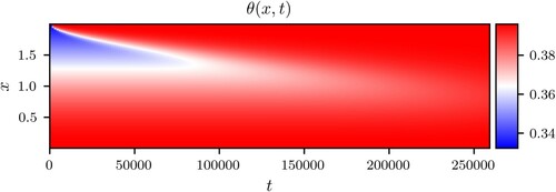
Figures 2 and 3 present the solution of the Richard's equation with the specified parameter values, boundary and initial conditions. Figure 2 presents the solution in terms of ψ, while Figure 3 presents the solution in terms of θ values.

Figure 2. Solution of the Richards equation in terms of ψ.

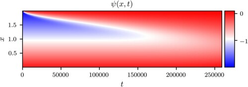
Figure 3. Solution of the Richards equation in terms of θ.

The inverse problem is formulated in this study as a problem in which a solution of the Richards equation is known at a given number of locations across the problem domain, ${\mathcal{T}}_i$, with the unknown solution of the Richards equation at the remaining locations, ${\mathcal{T}}_f$, of the problem domain and unknown values of input parameters $\mathit{\lambda }=[k_s,\alpha ,n{]}^T$. The values of ${\theta }_s$ and ${\theta }_r$ are assumed to be known. (32a) $\hat{\mathit{\lambda }}=\arg \underset{\mathit{\lambda }}{min}\left[\underset{\mathit{\chi }}{min}\mathcal{L}(\mathit{\chi },\mathit{\lambda }\mathcal{T})\right]$(32a) (32b) $\mathrm{subjected}\mathrm{to}:1\cdot {10}^{-9}[\mathrm{m}/\mathrm{s}]\le k_s\le 1\cdot {10}^{-7}[\mathrm{m}/\mathrm{s}]$(32b) (32c) $0.1[1/\mathrm{m}]\le \alpha \le 1[1/\mathrm{m}]$(32c) (32d) $1\le n\le 10$(32d)

4.1.1. Inner loop

The solution to the inverse problem in Equation (32) is found with a double loop optimisation algorithm. The inner loop of the algorithm aims to minimise the loss function in Equation (6(6) $\mathcal{L}(\mathit{\chi },\mathit{\lambda }\mathcal{T})=w_f{\mathcal{L}}_f(\mathit{\chi },\mathit{\lambda }{\mathcal{T}}_f)+w_b{\mathcal{L}}_b(\mathit{\chi },\mathit{\lambda }{\mathcal{T}}_b)+w_i{\mathcal{L}}_i(\mathit{\chi },\mathit{\lambda }{\mathcal{T}}_i)$(6) ) by adjusting the parameters of the neural network, $\mathit{\chi }$, for a given value of $\mathit{\lambda }$. The solution of the inner loop is an estimate of the solution of the Richards equation that satisfies the known values at ${\mathcal{T}}_i$ locations and the unknown values of the Richards equation at the rest of the domain, discretised into a set of ${\mathcal{T}}_f=40,000$ collocation points. The inner loop was implemented with the L-BFGS-B optimisation algorithm (Zhu et al., 1997) that is available in TensorFlow.

4.1.2. Outer loop

The outer loop aims to estimate an optimum value $\hat{\mathit{\lambda }}$ that minimises the loss function over a set of solutions of the Richards equation. The outer loop can be implemented with a wide range of optimisation algorithms. A relatively simple and robust global optimisation CE algorithm was implemented in this study for the outer loop. The CE is a population-based evolutionary algorithm for solving estimation and optimisation problems (De Boer et al., 2005). The CE solves an optimisation problem by updating a series of random search distributions such that the optimal or a near-optimal solution is more likely to be located. The random search distributions are updated in an adaptive process to converge to a distribution with high probability mass in the region of near-optimal solutions (Botev et al., 2013).

The CE algorithm with normal updating is implemented in this study. In the CE algorithm with normal updating, an independent normal random search distribution is assigned to each of the variables in $\mathit{\lambda }$. This results in a multivariate normal distribution with three independent components that are parametrised with a vector of means, ${\mathit{\mu }}_{\lambda }$, and a vector of variances, ${{\mathit{\sigma }}_{\lambda }}^2$. The CE algorithm iteratively updates ${\mathit{\mu }}_{\lambda }$ and ${{\mathit{\sigma }}_{\lambda }}^2$ by calculating them as the mean and variance of a subset of samples with the lowest values of $\mathcal{L}$ after each iteration. In the first iteration, the values of $\mathit{\lambda }$ were sampled uniformly from the ranges in Equation (32). In the following iterations, ${\mathit{\mu }}_{\lambda }$ and ${{\mathit{\sigma }}_{\lambda }}^2$ were calculated, respectively, as the mean and variance of the 50% quantile of samples with the lowest value of $\mathcal{L}$. The CE algorithm was implemented with 5 iterations and 10 samples in each iteration. The mean value, ${\mathit{\mu }}_{\lambda }$, calculated after the last iteration is adopted as an estimate of the optimum, $\hat{\mathit{\lambda }}$.

4.2. Pressure head formulation

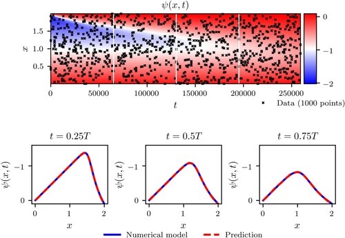
The pressure head PINN formulation was applied to an inverse problem in which ${\mathcal{T}}_i$ values of ψ are known at randomly selected locations across the model domain. The selected locations with known values of ψ are shown in Figure 4 with black crosses. In addition to satisfying the solution of the Richards equation at the locations with known values, the PINN aims to satisfy the solution in the rest of the domain by evaluating the loss ${\mathcal{L}}_f$ at a set of ${\mathcal{T}}_f=40,000$ collocation points that are distributed uniformly across the domain. As discussed earlier, the solution to the inverse problem is found with a double loop algorithm with the estimates of the unknown values of ψ at the collocation points and estimates of the unknown values of input parameters $\hat{\mathit{\lambda }}=[{\hat{k}}_s,\hat{\alpha },\hat{n}{]}^T$.

Figure 4. Inverse problem solution for the pressure head PINN formulation.

Figure 4 illustrates the performance of the pressure head PINN formulation on solving the inverse problem with ${\mathcal{T}}_i=1000$ randomly selected points with known values. The PINN approximation of the solution of the Richards equation at the collocation points is plotted behind the randomly selected points. A comparison between Figures 2 and 4 reveals that the PINN inverse solution and the numerical model solution agree very well. In order to further investigate the quality of the PINN approximation of the solution, the numerical solution and the PINN prediction are compared at several time instances in the lower part of Figure 4. The comparisons made at the time instances $0.25T$, $0.5T$, and $0.75T$ reveal good agreement between the numerical solution and the PINN prediction.

In addition to providing a prediction ψ at the collocation points, the solution to the inverse problem involves estimates of the unknown parameters $\hat{\mathit{\lambda }}=[{\hat{k}}_s,\hat{\alpha },\hat{n}{]}^T$. Estimates of the unknown parameters are provided in Table 1 for a range of ${\mathcal{T}}_i=\{500,1000,2000\}$. The values of ${\mathcal{T}}_i$ were varied to investigate the effects of the number of locations with known values of the solution of the inverse problem. In addition to the estimate parameter values, Table 1 presents the values of the losses ${\mathcal{L}}_i$ and ${\mathcal{L}}_f$ to provide an insight in the quality of the PINN prediction of the Richards equation across the domain, and the values of ${\mathit{\sigma }}_{\lambda }=[{\sigma }_{k_s},{\sigma }_{\alpha },{\sigma }_n{]}^T$ to examine the convergence of the CE algorithm.

Table 1. Loss values with the estimates of input parameters for a range of ${\mathcal{T}}_i$ values.

${\mathcal{T}}_i$	${\mathcal{L}}_i$	${\mathcal{L}}_f$	${\hat{k}}_s$ [m/s]	$\hat{n}$	$\hat{\alpha }$ [1/m]	${\sigma }_{k_s}$ [m/s]	${\sigma }_n$	${\sigma }_{\alpha }$ [1/m]
500	$3.05\cdot {10}^{-4}$	$4.02\cdot {10}^{-13}$	$6.498\cdot {10}^{-8}$	5.896	0.569	$1.137\cdot {10}^{-8}$	1.017	0.126
1000	$3.86\cdot {10}^{-4}$	$2.67\cdot {10}^{-12}$	$7.044\cdot {10}^{-8}$	$4.213$	$0.547$	$1.055\cdot {10}^{-9}$	0.697	0.102
2000	$2.842\cdot {10}^{-4}$	$8.455\cdot {10}^{-13}$	$7.206\cdot {10}^{-8}$	$5.512$	$0.5638$	$7.815\cdot {10}^{-9}$	0.796	0.096

From the values of ${\mathcal{L}}_i$ and ${\mathcal{L}}_f$ in Table 1, it can be seen that the PINN provides good prediction of the solution to the pressure head formulation of the Richards equation with ${\mathcal{L}}_i\approx {10}^{-4}$ and ${\mathcal{L}}_f\approx {10}^{-13}$. The number of locations with known values of the solution does not significantly affect the losses. The values of the estimated input parameters $\hat{\mathit{\lambda }}=[{\hat{k}}_s,\hat{\alpha },\hat{n}{]}^T$ reveal a relatively good agreement with the actual input values. This is reflected in the actual and predicted values of $k_s$ and α being relatively close. The estimated values of n show somewhat less good agreement with the predicted values approximately from 4 to 6 and the actual value of 2.06. Some of the potential reasons this disagreement may be from the value of n being less influential in the optimisation process or the CE algorithm requiring additional iterations to converge to a more optimal solution. Additional iterations would be beneficial for increasing the prediction accuracy of the CE algorithm, with the ratio of standard deviation of the estimates over the mean being between 10% and 20% in Table 1. The CE algorithm was implemented in this study with relatively low 5 iterations as a compromise between accuracy and computational time.

The capacity of the PINN to solve the inverse problem with noisy data was investigated by adding normally distributed error to the dataset. The error term is defined as a normally distributed random variable with zero mean and standard deviation of ${\sigma }_e\cdot {\sigma }_d$, where ${\sigma }_d$ is the standard deviation of the dataset. Figure 5 shows the performance of the pressure head PINN formulation on the inverse problem with noisy data. The data consist of the ${\mathcal{T}}_i=1000$ randomly selected points with known ψ values, while the noise is specified by ${\sigma }_e=0.05$.

Figure 5. Inverse problem solution for the pressure head PINN formulation with noisy data and ${\sigma }_e=0.05$.

From Figures 5 and 2, it can be observed that the provided solution of the Richards equation agrees very well with the original noise-free solution of the numerical model. The quality of the PINN approximation of the solution with a noisy dataset is further investigated in Figure 5 by comparing the noise-free numerical solution and the PINN prediction at several time instances. The comparisons made at the time instances $0.25T$, $0.5T$ and $0.75T$ reveal very good agreement between the noise-free numerical solution and the PINN prediction. These results demonstrate the capacity of PINNs to solve noise inverse problems and identify the original noise-free solution of the Richards equation despite the dataset being subjected moderate amounts of noise.

The effects of the noise level in the dataset on the capacity of the PINN pressure head formulation on solving the inverse problem is investigated for a range of ${\sigma }_e=\{0.025,0.05,0.075\}$ in Table 2 with ${\mathcal{T}}_i=1000$. The results indicate that the quality of the prediction over the problem domain decreases with increasing noise levels from ${\mathcal{L}}_i\approx {10}^{-4}$ and ${\mathcal{L}}_f\approx {10}^{-12}$ for ${\sigma }_e=0.025$ to ${\mathcal{L}}_i\approx {10}^{-3}$ and ${\mathcal{L}}_f\approx {10}^{-10}$ for ${\sigma }_e=0.075$. The estimates of the input parameters do not show significant variations due to increasing noise levels. Further increasing noise revels result in the solution not converging or showing great deviations from the noise-free solution due to overfitting. Among the estimated values, $k_s$ and α show a relatively good agreement with the input values, while the estimates of n show higher deviations from the input values. As discussed earlier, some of the potential reasons these deviations may be from the value of n being less influential in the optimisation process or the CE algorithm requiring additional iterations to converge to a more optimal solution.

Table 2. Loss values with the estimates of input parameters for a range of ${\sigma }_e$ values.

${\sigma }_e$	${\mathcal{L}}_i$	${\mathcal{L}}_f$	${\hat{k}}_s$ [m/s]	$\hat{n}$	$\hat{\alpha }$ [1/m]	${\sigma }_{k_s}$ [m/s]	${\sigma }_n$	${\sigma }_{\alpha }$ [1/m]
0.025	$3.548\cdot {10}^{-4}$	$1.408\cdot {10}^{-12}$	$7.107\cdot {10}^{-8}$	$5.238$	$0.547$	$1.083\cdot {10}^{-8}$	0.363	0.058
0.05	$3.638\cdot {10}^{-4}$	$1.975\cdot {10}^{-12}$	$5.202\cdot {10}^{-8}$	4.802	0.296	$1.095\cdot {10}^{-8}$	0.545	0.267
0.075	$7.155\cdot {10}^{-3}$	$3.664\cdot {10}^{-10}$	$5.243\cdot {10}^{-8}$	$3.923$	$0.601$	$2.727\cdot {10}^{-8}$	0.525	0.107

4.3. Volumetric water content formulation

The VWC PINN formulation was applied to an inverse problem in which ${\mathcal{T}}_i$ values of θ are known at randomly selected locations across the model domain. The selected locations with known values of θ are shown in Figure 6 with black crosses. In addition to satisfying the solution of the Richards equation at the locations with known values, the PINN aims to satisfy the solution in the rest of the domain by evaluating the loss ${\mathcal{L}}_f$ at a set of ${\mathcal{T}}_f=40,000$ collocation points that are distributed uniformly across the domain. Similar as for the pressure head formulation, the solution to the inverse problem is found with a double loop algorithm with the estimates of the unknown values of θ at the collocation points and estimates of the unknown values of input parameters $\hat{\mathit{\lambda }}=[{\hat{k}}_s,\hat{\alpha },\hat{n}{]}^T$.

Figure 6. Inverse problem solution for the VWC-PINN formulation.

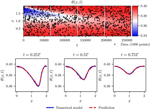
Figure 6 shows the performance of the VWC PINN formulation on solving the inverse problem with ${\mathcal{T}}_i=1000$ randomly selected points with known values. A comparison between Figures 3 and 6 reveals that the PINN inverse solution and the numerical model solution agree very well. Further investigation of the prediction quality is conducted in the lower part of Figure 6 by comparing the PINN approximation of the solution and the numerical solution at several time instances. The comparisons made at the time instances $0.25T$, $0.5T$ and $0.75T$ reveal good agreement between the numerical solution and the PINN prediction with some deviations in the proximity of the upper bound $x_1$.

Estimates of the unknown parameters $\hat{\mathit{\lambda }}=[{\hat{k}}_s,\hat{\alpha },\hat{n}{]}^T$ are provided in Table 3 for a range of ${\mathcal{T}}_i=\{500,1000,2000\}$. Table 3 also presents the values of the losses ${\mathcal{L}}_i$ and ${\mathcal{L}}_f$ to provide an insight in the quality of the PINN prediction of the Richards equation across the domain, and the values of ${\mathit{\sigma }}_{\lambda }=[{\sigma }_{k_s},{\sigma }_{\alpha },{\sigma }_n{]}^T$ to examine the convergence of the CE algorithm.

Table 3. Loss values with the estimates of input parameters for a range of ${\mathcal{T}}_i$ values.

${\mathcal{T}}_i$	${\mathcal{L}}_i$	${\mathcal{L}}_f$	${\hat{k}}_s$ [m/s]	$\hat{n}$	$\hat{\alpha }$ [1/m]	${\sigma }_{k_s}$ [m/s]	${\sigma }_n$	${\sigma }_{\alpha }$ [1/m]
500	$1.769\cdot {10}^{-6}$	$1.372\cdot {10}^{-9}$	$7.820\cdot {10}^{-8}$	5.806	0.623	$9.734\cdot {10}^{-9}$	2.279	0.068
1000	$1.560\cdot {10}^{-6}$	$1.405\cdot {10}^{-9}$	$5.776\cdot {10}^{-8}$	$7.005$	$0.586$	$1.125\cdot {10}^{-9}$	1.127	0.063
2000	$3.644\cdot {10}^{-6}$	$7.444\cdot {10}^{-9}$	$8.511\cdot {10}^{-8}$	$4.617$	$0.578$	$4.527\cdot {10}^{-9}$	3.700	0.067

From the values of ${\mathcal{L}}_i$ and ${\mathcal{L}}_f$ in Table 3, it can be seen that the PINN provides good prediction of the solution to the VWC formulation of the Richards equation with ${\mathcal{L}}_i\approx {10}^{-6}$ and ${\mathcal{L}}_f\approx {10}^{-9}$. The values of the estimated input parameters $\hat{\mathit{\lambda }}=[{\hat{k}}_s,\hat{\alpha },\hat{n}{]}^T$ reveal a relatively good agreement with the actual input values. Similar as for the pressure head PINN formulation results, the estimated values of n show somewhat less good agreement with the predicted values approximately from 4 to 7.

The capacity of the VWC PINN to solve the inverse problem with noisy data was investigated by adding normally distributed error to the dataset as for the pressure head formulation. Figure 7 shows the performance of the pressure head PINN formulation on the inverse problem with noisy data. The data consist of the ${\mathcal{T}}_i=1000$ randomly selected points with known ψ values, while the noise is specified by ${\sigma }_e=0.04$.

Figure 7. Inverse problem solution for the VWC-PINN formulation with a noisy data, specified with ${\sigma }_e=0.04$.

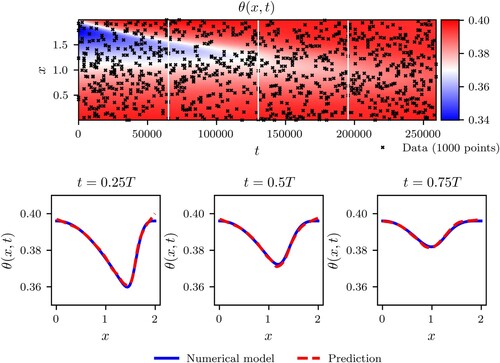
Comparison of Figures 7 and 3 shows that the provided solution of VWC formulation agrees very well with the original noise-free solution of the numerical model. The quality of the VWC PINN approximation of the solution with a noisy dataset is further investigated in Figure 7 by comparing the noise-free numerical solution and the PINN prediction at several time instances. The comparisons made at the time instances $0.25T$, $0.5T$ and $0.75T$ reveal very good agreement between the noise-free numerical solution and the VWC PINN prediction. These results demonstrate the capacity of the VWC PINN formulation to solve noise inverse problems and identify the original noise-free solution of the Richards equation despite the dataset being subjected moderate amounts of noise.

The effects of the noise level in the dataset on the capacity of the PINN VWC formulation on solving the inverse problem are investigated for a range of ${\sigma }_e=\{0.02,0.04,0.06\}$ in Table 4 with ${\mathcal{T}}_i=1000$. The results indicate that the quality of the prediction is not significantly affected by the increasing noise levels with ${\mathcal{L}}_i\approx {10}^{-}6$ and ${\mathcal{L}}_f\approx {10}^{-9}$ for the examined noise levels. Similar to the pressure head formulation, further increasing noise revels result in the solution not converging or showing great deviations from the noise-free solution due to over-fitting. The estimates of the input parameters do not show significant variations due to increasing noise levels. Similar as for the earlier analyses, the estimates n show higher deviations from the input values.

Table 4. Loss values with the estimates of input parameters for a range of ${\sigma }_e$ values.

${\sigma }_e$	${\mathcal{L}}_i$	${\mathcal{L}}_f$	${\hat{k}}_s$ [m/s]	$\hat{n}$	$\hat{\alpha }$ [1/m]	${\sigma }_{k_s}$ [m/s]	${\sigma }_n$	${\sigma }_{\alpha }$ [1/m]
0.01	$1.151\cdot {10}^{-6}$	$1.019\cdot {10}^{-9}$	$4.207\cdot {10}^{-8}$	4.269	0.449	$2.591\cdot {10}^{-9}$	0.479	0.148
0.02	$2.185\cdot {10}^{-6}$	$2.208\cdot {10}^{-9}$	$6.057\cdot {10}^{-8}$	$5.895$	$0.342$	$1.417\cdot {10}^{-8}$	0.236	0.122
0.04	$1.456\cdot {10}^{-6}$	$9.987\cdot {10}^{-10}$	$5.534\cdot {10}^{-8}$	$4.669$	$0.477$	$2.036\cdot {10}^{-8}$	0.943	0.161

5. Water-infiltration test

5.1. Test setup

The performance of the VWC PINN formulation for the Richards equation is further investigated by solving the inverse problem on a dataset from a water infiltration test. A large-scale water infiltration test was conducted to study the infiltration process in unsaturated soil by using instrumentation and visual interpretation (Robinson, 2019), as shown in Figure 8. The column was designed with reference to the ASTM D7664-10: Standard Test Methods for Measurements of Hydraulic Conductivity of Unsaturated Soils (ASTM, 2010) and infiltration tests performed in McCartney, Villar, and Zornberg (2007), Li, Zhang, and Fredlund (2009), and Duong et al. (2013).

Figure 8. Water infiltration column setup with the PINN prediction of the solution and comparisons with the measurements.

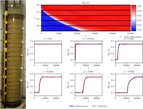
The infiltration test consists of a 1-m-high soil column placed within a hollow acrylic cylinder. The cylinder is 1.3 m high with the outer diameter of 0.25 m and the inner diameter of 0.24 m. The remaining 0.3 m above the soil level was used to maintain a constant pressure head of 0.1 m for the duration of the infiltration test. The column was placed on the base assembly to prevent water leakage and a valve to control the boundary conditions at the base. The valve can be opened to allow for water drainage or closed to simulate an impervious base. A filter system was installed on the contact between the soil and the base to minimise fines migration and support the soil column. Similarly, a stainless steel perforated plate and filter cloth were placed on top of the soil column to reduce soil disturbance during the initial stages of water filling. The constant water head of 0.1 m on top of the soil column was maintained with a custom water supply system, as shown in Figure 8.

The soil mixture for the infiltration test was created from a combination of three soils to obtain a soil mixture that was representative of some Norwegian moraine soils. The resulting mixture had approximately 9% of clay fines, 46% of silty fines, with the rest being sand fractions. The soil was placed into the column in 0.05 m lifts and compacted to the density of 1415 kg/m${}^3$ with a volumetric water content of $\theta =0.0991$. While placing the soil into the column, a set of volumetric water content sensors were installed vertically at five positions. The positions of sensors are from the top at $x=[0.15,0.3,0.45,0.6,0.75]$ m. In addition to the measured values of VWC at the location of the sensors, the values of VWC are assumed to be known at the top and correspond to ${\theta }_s$. The experiment was conducted for $T=250,000$  s. Figure 8 shows the conditions shortly after the start of the water infiltration column test with the top 0.05 m being saturated, as observed by the darker soil colour.

5.2. Inverse analysis

The collected VWC measurements will be used in the PINN-based inverse analysis to estimate the parameters of the van Genuchten model and predict VWC at the non-measured spatio-temporal instances as modelled by the Richards PDE. The values of ${\theta }_r=0.0991$ and ${\theta }_s=0.35$ are determined from preliminary laboratory tests conducted in Robinson (2019) with the values of $k_s$, α and n to be determined from the analysis.

Given the measurements from the VWC sensors, the VWC PINN formulation was adopted for the implementation of the inverse problem. As introduced earlier, the inverse problem is formulated as a problem in which a solution of the Richards PDE is known at the locations of the VWC sensors for the duration of the test. The temporal domain was discretised into 501 points, which results in ${\mathcal{T}}_i=3006$ points with known VWC values. The spatial domain was discretised into 76 points, with the total number of collocation points being ${\mathcal{T}}_f=38,076$. The inverse problem for the water infiltration tests is specified as follows with the bounds on $k_s$, α and n selected from Robinson (2019): (33a) $\hat{\mathit{\lambda }}=\arg \underset{\mathit{\lambda }}{min}\left[\underset{\mathit{\chi }}{min}\mathcal{L}(\mathit{\chi },\mathit{\lambda }\mathcal{T})\right]$(33a) (33b) $\mathrm{subjectedto}:1\cdot {10}^{-7}[\mathrm{m}/\mathrm{s}]\le k_s\le 1\cdot {10}^{-5}[\mathrm{m}/\mathrm{s}]$(33b) (33c) $0.1[1/\mathrm{m}]\le \alpha \le 1.5[1/\mathrm{m}]$(33c) (33d) $1\le n\le 15$(33d) The solution to the inverse problem in Equation (33) is found by implementing a PINN based on the VWC formulation and the double-loop algorithm introduced earlier. The PINN has eight layers with the first layer having two neurons and the output layer a single neuron. The remaining 6 layers have 50 neurons each. Relu activation function was selected as it was found to provide the most stable results.

5.3. Results

Results of the inverse problem for the water infiltration column test are presented in Figure 8. The left part of Figure 8 presents the setup of the water infiltration column test, with the right part presenting the solution of the inverse problem. In addition to providing predictions of the Richards PDE across the problem domain, the solution of the inverse problem involves estimates of the van Genuchten model parameters $\mathit{\lambda }=[k_s,\alpha ,n{]}^T$. The following estimates were made with ${\hat{k}}_s=2.256\cdot {10}^{-7}$ [m/s], $\hat{\alpha }=0.948$ [1/m] and $n=7.824$. These values of the model parameters were associated with the loss values of ${\mathcal{L}}_i=8.937\cdot {10}^{-6}$ and ${\mathcal{L}}_f=3.960\cdot {10}^{-5}$. The PINN prediction in Figure 8 is calculated based on these estimates of the van Genuchten model parameters.

The right side of Figure 8 presents the locations of the points with known values of VWC and the approximation of the solution of the Richards PDE at locations with no measurements on the upper plot. The locations of the points with known values of VWC are shown with black markers and correspond to the top surface and the locations of the VWC sensors. The resulting solution indicated that there is a relatively rapid transition from unsaturated to saturated conditions in the upper 0.2 m of the model. The infiltration of water to the deeper layers of soil slows down somewhat with the soil column becoming saturated before 200,000 s.

In addition to presenting the solution of the Richards PDE across the problem domain, a set of six graphs is presented in the lower right part of Figure 8 to compare the PINN predictions of θ and the known or measured values. The top three graphs show the known or measured values of θ in comparison to the values predicted by PINN at depths of 0, 0.15 and 0.3 m. These graphs demonstrate that there is a very rapid and sharp transition from unsaturated to saturated conditions in the upper part of the column. The capacity of the PINN to capture the rapid and sharp transitions observed in the measurements is conformed with a relatively good agreement between the PINN predictions and the measurements. Closer inspection of the transitions reveals that the PINN predictions are somewhat smoother than the measurements.

The lower three graphs in the right part of Figure 8 compare the PINN prediction with the measurements of θ at the depths of 0.45, 0.6 and 0.75 m. These graphs show that the transitions from unsaturated to saturated conditions are less rapid with the transition being diffused in comparison to the shallower depths. The PINN predictions agree very well with the measurements thus showing a good capacity to approximate the highly nonlinear infiltration process, as modelled by the Richards PDE and the van Genuchten model. Similar to the approximations of sharp transitions at shallower depths, some smoothing occurs in the PINN approximation of the sharp transitions that appear as the water first approaches the locations of the VWC sensors.

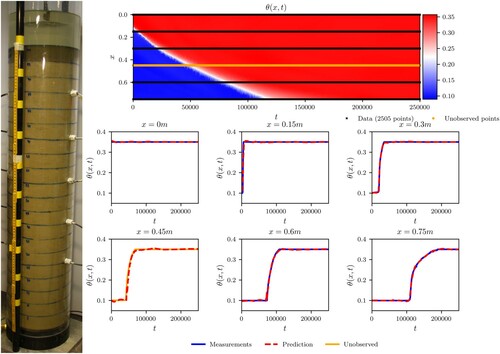
To further investigate the generalisation capability and the physical plausibility of the trained PINN, data collected from one of the sensors were excluded from the training dataset and used to validate PINN's predictive capacity. Figure 9 shows the performance of the PINN with the data from the sensor at position x = 0.45 m being excluded from the training dataset. The resulting predictions of the PINN demonstrate very good predictive capacity of the trained PINN both on the training dataset and the unobserved data. As observed from Figures 8 and 9, the PINN approximates the shock behaviour very well. This can be attributed to the use of the ReLU activation function, which was selected among the various activation functions due to its capacity to predict sharp changes in the solutions of the Richards equation.

Figure 9. Water infiltration column setup with the PINN prediction of the solution and comparisons with the measurements and unobserved data.

6. Discussion

This study investigated the applications of PINNs to the Richards PDE and the van Genuchten model. PINNs have been successfully applied to solve forward and backward problems for various PDEs, benefiting from the DNNs capacity to approximate complex functions and the computational efficiency of AD to evaluate partial derivatives of the PINN predictions with respect to model parameters, which is used to enforce the PDE on a set of collocation points. This paper specifically focused on the Richards PDE with the van Genuchten model due to the van Genuchten model being often used in analysing groundwater flow in unsaturated soils. The adoption of the van Genuchten model in this study allowed for an implementation of a PINN with only one DNN and analytical derivations of WRC and HCF.

Although PINNs can be applied to both the forward and inverse problems for various types of PDEs, this paper investigated the application of PINNs only for the inverse problem with the Richards PDE. One of the main reason for this limitation is the nonlinearity of the Richards PDE with the van Genuchten model, which can lead to difficulties in reliably converging to an accurate solution. Several analyses, conducted as a part of this study, on the PINN solution to the forward problem with the Richards PDE and the van Genuchten model showed promising results. However, due to the inability to consistently converge to relatively accurate solutions they were not presented in this study. Conversely, the focus is on PINN solution to the inverse problem due the capacity of PINNs to provide solutions with relatively high accuracy and high computational efficiency.

The inverse problem is postulated in this study as a problem where the solutions of the Richards PDE are known at a given set of spatio-temporal instances with the unknown values at the remaining instances and unknown parameters of the van Genuchten model. A highly efficient solution to an inverse problem can be obtained with PINNs by utilising the AD in the process of finding the optimal solution and parameter values that minimise the loss function. However, such implementations resulted in sub-optimal performance in this study with the algorithm minimising the loss function not being able to efficiently advance among the values of the van Genuchten model parameters. This resulted in the inverse solution resulting in sub-optimal solutions or physically inconsistent values. This is attributed to the nonlinearity and complexity of the Richards PDE with the van Genuchten model. A double loop algorithm was implemented in this study to overcome this challenge, with the inner loop optimising the parameters of the DNN and the outer loop optimising the van Genuchten parameters. Constraints and bounds on the van Genuchten parameters are enforced on the outer loop, which was implemented with the CE global optimisation algorithm. The double loop algorithm is implemented as a compromise between computational efficiency and the solution accuracy and stability.

This study features the pressure head and the VWC formulations of PINNs for the Richards PDE with the van Genuchten model to adapt to situations in which, respectively, the pressure head and VWC measurement are available. For both of the formulations, the Richards PDE was expressed in terms of the respective variable (i.e. pressure head or VWC) with the partial derivatives of the variable reformulated in terms of analytical expressions and the derivatives of the variables with respect to time or space. The analytical expressions are derived based on the van Genuchten model, while the derivative of pressure head or VWC with respect to time and space are evaluated with the AD based on the PINN prediction. This allows the PINN for the Richards PDE and the van Genuchten model to be efficiently implemented with a single DNN.

The performance of PINNs for the inverse problem with the Richards PDE and the van Genuchten model was investigated on synthetically generated measurements and the dataset from a water infiltration column test. The synthetically generated data were used to evaluate the performance of both the PINN formulations for a range of available measurements and noise levels. The results demonstrated good performance for both formulations with relatively low effect of the number of measurements on the accuracy for the considered range. Relatively similar estimates of saturated permeability in the van Genuchten model were obtained for all analyses, with higher variation of α values and some deviations for n. This might indicate that n is less influential in the optimisation process or that additional iterations of the CE algorithm could have been implemented. The effects of noise in the measurements on the solution to the inverse problems showed that PINNs can deal with low to medium noise levels and identify the original non-noisy solution. Higher noise levels result in the lack of convergence or great deviations from the original solution due to over-fitting. The VWC PINN formulation was applied to VWC measurements for a water infiltration column test to predict the solution of the Richards equation at non-measured spatio-temporal instances and estimate parameters of the van Genuchten model. The results demonstrate that PINNs are capable of providing a very good prediction of the solution to the Richards equation based on realistic data and a very good fit to highly nonlinear and sharp transitions from unsaturated to saturated conditions that are observed in the measurements.

PINNs represent a hybrid modelling approach that bridges the gap between physical-based (e.g. FEM, FDM) and data-driven approaches. Hybrid approaches aim to integrate the advantages of both approaches with the capacity of data-driven approaches to efficiently integrate and process large amounts of data and for the solution to satisfy the physical laws as described by the governing PDEs. These unique modelling capabilities of PINNs allow it to find applications in situations where large amounts of data are available and physical interpretability of the data or predictions based on those data are important. One such application involves real-time monitoring systems.

Real-time monitoring systems are one of commonly employed strategies for managing geohazards risks, which aims to reduce the risks by issuing timely alerts to evacuate people and property under risk. Real-time monitoring systems often feature large numbers of sensors that produce data time series that require efficient interpretation and processing. Hybrid approaches can contribute to the implementation of such systems with the capacity to efficiently process large amounts of data collected through monitoring system and simultaneously be used to provide predictions of natural phenomena that are based on physical laws described by the governing PDEs. Physical interpretability of collected data and model predictions is of great importance in supporting a decision-making process that is necessary for the implementation of reliable warning systems.

7. Conclusion

This study investigated the application of physics-informed neural networks to the inverse problem for the Richards partial differential equation with the van Genuchten model. Pressure head and volumetric water content formulations of physics-informed neural networks were developed to adapt to situations in which the respective measurements are available. The implementation of the two formulations requires only one deep neural network to be trained due to analytical derivations of partial derivations in the Richards equation based on the van Genuchten model. The two formulations were successfully implemented on several examples to demonstrate the capacity of physics-informed neural networks to provide accurate predictions of the inverse solution to the Richards equation and to determine the parameters of the van Genuchten model.

Acknowledgements

The authors acknowledge the use of the publicly available code for physics-informed neural networks from Maziar Raissi in the development of this study and the valuable contributions from Kate Robinson in implementing the water infiltration column test.

Disclosure statement

No potential conflict of interest was reported by the author(s).

References

- Abadi, Martín, Ashish Agarwal, Paul Barham, Eugene Brevdo, Zhifeng Chen, Craig Citro, and Greg S. Corrado. 2015. “TensorFlow: Large-Scale Machine Learning on Heterogeneous Systems.” Software Available from tensorflow.org, http://tensorflow.org/.
- Abkenar, Fatemeh Zakizadeh, Ali Rasoulzadeh, and Ali Asghari. 2019. “Performance Evaluation of Different Soil Water Retention Functions for Modeling of Water Flow Under Transient Condition.” Bragantia 78: 119–130.
- ASTM. 2010. ASTM D7664 – 10 Standard Test Methods for Measurement of Hydraulic Conductivity of Unsaturated Soils. Technical Report. ASTM. https://www.astm.org/DATABASE.CART/HISTORICAL/D7664-10.htm.
- Bandai, Toshiyuki, and Teamrat Ghezzehei. 2020. “Physics-Informed Neural Networks for Richardson-Richards Equation: Estimation of Constitutive Relationships and Soil Water Flux Density From Volumetric Water Content Measurements.” Earth and Space Science Open Archive.
- Botev, Zdravko I., Dirk P. Kroese, Reuven Y. Rubinstein, and Pierre L'Ecuyer. 2013. “The Cross-Entropy Method for Optimization.” In Handbook of Statistics. Vol. 31, 35–59. Chennai: Elsevier.
- Chen, Yuyao, Lu Lu, George Em Karniadakis, and Luca Dal Negro. 2020. “Physics-Informed Neural Networks for Inverse Problems in Nano-Optics and Metamaterials.” Optics Express 28 (8): 11618–11633.
- De Boer, Pieter-Tjerk, Dirk P. Kroese, Shie Mannor, and Reuven Y. Rubinstein. 2005. “A Tutorial on the Cross-Entropy Method.” Annals of Operations Research 134 (1): 19–67.
- Depina, Ivan, Emir Ahmet Oguz, and Vikas Thakur. 2020. “Novel Bayesian Framework for Calibration of Spatially Distributed Physical-Based Landslide Prediction Models.” Computers and Geotechnics 125: 103660.
- Duong, Trong Vinh, Viet Nam Trinh, Yu-Jun Cui, Anh Minh Tang, and Nicolas Calon. 2013. “Development of A Large-Scale Infiltration Column for Studying the Hydraulic Conductivity of Unsaturated Fouled Ballast.” Geotechnical Testing Journal 36 (1): 54–63.
- Ireson, Andrew. October, 2020. “1D Richards' Equation Model.” https://github.com/amireson/RichardsEquation, https://github.com/amireson/RichardsEquation.
- Li, X., L. M. Zhang, and D. G. Fredlund. 2009. “Wetting Front Advancing Column Test for Measuring Unsaturated Hydraulic Conductivity.” Canadian Geotechnical Journal 46 (12): 1431–1445.
- Lu, Lu, Xuhui Meng, Zhiping Mao, and George E. Karniadakis. 2019. “DeepXDE: A Deep Learning Library for Solving Differential Equations.” ArXiv preprint arXiv:1907.04502.
- McCartney, J. S., L. Villar, and J. G. Zornberg. 2007. “Estimation of the Hydraulic Conductivity Function of Unsaturated Clays Using an Infiltration Column Test.” In Proceedings of the 6th Brazilian Conference on Unsaturated Soils (NSAT). Vol. 1, 321–328. Salvador, Brazil.
- Mishra, Siddhartha, and Roberto Molinaro. 2021. “Estimates on the Generalization Error of Physics-Informed Neural Networks for Approximating a Class of Inverse Problems for PDEs.” IMA Journal of Numerical Analysis.
- Paszke, Adam, Sam Gross, Francisco Massa, Adam Lerer, James Bradbury, Gregory Chanan, and Trevor Killeen, et al. 2019. “PyTorch: An Imperative Style, High-Performance Deep Learning Library.” In Advances in Neural Information Processing Systems 32, edited by H. Wallach, H. Larochelle, A. Beygelzimer, F. dAlche Buc, E. Fox, and R. Garnett, 8024–8035. Curran Associates, Inc. http://papers.neurips.cc/paper/9015-pytorch-an-imperative-style-high-performance-deep-learning-library.pdf.
- Rai, Pankaj Kumar, and Shivam Tripathi. 2019. “Gaussian Process for Estimating Parameters of Partial Differential Equations and Its Application to the Richards Equation.” Stochastic Environmental Research and Risk Assessment 33 (8-9): 1629–1649.
- Raissi, Maziar, Paris Perdikaris, and George E. Karniadakis. 2019. “Physics-Informed Neural Networks: A Deep Learning Framework for Solving Forward and Inverse Problems Involving Nonlinear Partial Differential Equations.” Journal of Computational Physics 378: 686–707.
- Richards, Lorenzo Adolph. 1931. “Capillary Conduction of Liquids Through Porous Mediums.” Physics 1 (5): 318–333.
- Robinson, Kate. 2019. “Experimental and Numerical Investigations of Infiltration into Unsaturated Soil.” Master's Thesis, NTNU. http://hdl.handle.net/11250/2631811.
- Rumelhart, David E., Geoffrey E. Hinton, and Ronald J. Williams. 1986. “Learning Representations by Back-Propagating Errors.” Nature 323 (6088): 533–536.
- Schindler, Uwe Georg, and Lothar Müller. 2017. “Soil Hydraulic Functions of International Soils Measured with the Extended Evaporation Method (EEM) and the HYPROP Device.” Open Data Journal for Agricultural Research 3.
- Šimunek, J, M. Th. Van Genuchten, and M. Šejna. 2012. “The HYDRUS Software Package for Simulating the Two-and Three-Dimensional Movement of Water, Heat, and Multiple Solutes in Variably-Saturated Porous Media.” Technical Manual.
- Tartakovsky, Alexandre M., Carlos Ortiz Marrero, Paris Perdikaris, Guzel D. Tartakovsky, and David Barajas-Solano. 2018. “Learning Parameters and Constitutive Relationships with Physics Informed Deep Neural Networks.” ArXiv Preprint arXiv:1808.03398.
- Van Genuchten, M. Th. 1980. “A Closed-Form Equation for Predicting the Hydraulic Conductivity of Unsaturated Soils.” Soil Science Society of America Journal 44 (5): 892–898.
- Zhang, Lulu, Fang Wu, Yafei Zheng, Lihong Chen, Jie Zhang, and Xu Li. 2018. “Probabilistic Calibration of a Coupled Hydro-Mechanical Slope Stability Model with Integration of Multiple Observations.” Georisk: Assessment and Management of Risk for Engineered Systems and Geohazards 12 (3): 169–182.
- Zhu, Ciyou, Richard H. Byrd, Peihuang Lu, and Jorge Nocedal. 1997. “Algorithm 778: L-BFGS-B: Fortran Subroutines for Large-Scale Bound-Constrained Optimization.” ACM Transactions on Mathematical Software (TOMS) 23 (4): 550–560.