What is a characteristic value for soils?

ABSTRACT

The choice of the characteristic value of a material property is fundamental in all civil engineering design and critical in geotechnical engineering. Based on our tradition, we strive to look for a cautious value, whose evaluation includes our engineering judgement. While the definition of a characteristic value is often given with the aid of statistics as a fractile value, its determination includes considerations of mechanics because “value” refers to the relevant quantity affecting the limit state. Soils are complex, often spatially heterogeneous and our knowledge of them is typically based on sparse incomplete data. This makes the definition and determination of a characteristic value for soils more multifaceted than for structural materials. This paper discusses the choice of the characteristic value for soils from various perspectives (statistical, mechanistic and practical) and summarises some recent findings to clarify the limitations of existing practice. Overly simplified statistical approaches may lead to unsafe or overly conservative designs. The authors conclude that a balance between practicality and incorporating salient features are needed. By increasing the value of data in design decisions, engineers will be motivated to collect, share, and utilise data as much as possible and bring our practice closer to the digital economy.

KEYWORDS:

• Eurocode
• statistics-based characteristic value
• reliability-based characteristic value
• mobilisation-based characteristic value
• weakest-path model

1. Introduction

According to the Webster’s Encyclopedic Unabridged Dictionary of the English language the word characteristic has the meaning “pertaining to, constituting, or indicating the character or peculiar quality of a person or thing; typical; distinctive”. A characteristic value for a material property could thus be seen as a typical value that truly represents the material and describes its fundamental quality.

In civil engineering design we often wish to be cautious in our design assumptions. For example, when picking a material value, if we do not know the exact value and we do not know how to handle the uncertainty (a range of test results) explicitly, it is reasonable to pick a cautious value that is affected by the lower bound, rather than an average that is less affected by the lower bound. This is often considered as part of engineering judgement. Engineering judgment and cautious estimates based on judgment are though difficult to quantify. When writing standards, it might be seen as desirable, to put clear numbers and equations to provide a data-informed basis from which engineering judgment could be applied to decide how cautious a characteristic value should be. In addition, making effective judgment without a data-informed basis is increasingly difficult as big data increase in volume, velocity (or rate), and variety. Depending on the experience of the engineer, one can imagine a situation where pure engineering judgment arrives at a characteristic value that is significantly at odds with what the data is saying.

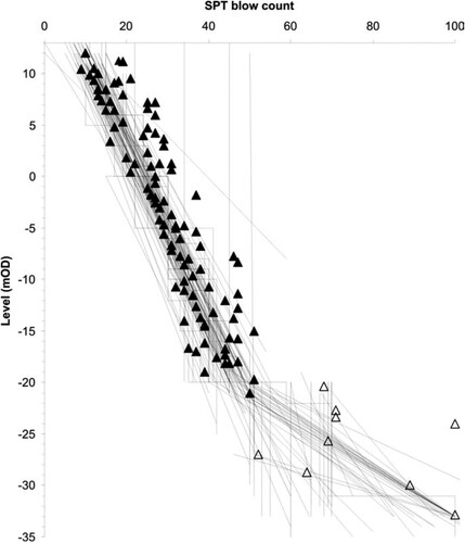
The problem was clearly illustrated by Bond and Harris (2008), presenting results of a study where more than one hundred engineers and engineering geologists were asked to select a characteristic line (or lines) based on more than one hundred standard penetration tests performed at a site in Holborn, London, as shown in Figure 1. In the upper part (London clay, above approx. −21 m OD) there seems to be relatively good consensus about the trend, although the results are rather widespread, and some estimates deviate greatly from the average interpretation. For the lower part (Lambeth clay) where the data is more scattered, also the interpretations vary widely.

Figure 1. Results of standard penetration tests in London and Lambeth clays, with engineers’ interpretation of the characteristic value (Bond and Harris 2008).

In this paper, the problem of defining characteristic values for soils is discussed with respect to the Eurocodes and geotechnical design standards in general. Important recent findings that cover statistical, mechanistic and practical perspectives are reviewed to clarify limitations of existing practice. The authors are of the opinion that simple equations consistent with the qualitative guidelines provided in Eurocode 7 (EN 1997-1; CEN 2004) can be developed to account appropriately for spatial variability, failure mechanism, and their interactions correctly.

2. Characteristic values in the Eurocodes

2.1. General

In the Eurocode system, as in many other standards, the design value of a material property or resistance is obtained by dividing the characteristic value by a partial safety factor. According to EN 1990 “When a limit state verification is sensitive to the variability of a material property, upper and lower characteristic values of the material property should be taken into account.” (CEN 2002). EN 1990 further states that unless otherwise stated in the material codes, a 5% fractile value should be used for a low value of material property and a 95% fractile value for a high value material property. For the structural stiffness parameters, EN 1990 states that they should normally be represented by mean values.

EN 1997–1 states that “The characteristic value of a geotechnical parameter shall be selected as a cautious estimate of the value affecting the occurrence of the limit state.” Although this complies with EN 1990, there are some underlying differences when selecting this value as the characteristic value for geotechnical design, as also pointed out by Simpson and Driscoll (1998). In structural design, the choice of a characteristic value is more straightforward and can often be based on statistical procedures applied to the results of material tests. In geotechnical design one firstly needs to identify what the materials (soils and rock) are. This is often guided by experience and existing geological data. Field and laboratory investigations are then used to verify the identification and specify the properties more accurately. Often it is advisable to carry out the investigations in two or more rounds. Still, only a small fraction of the relevant ground volume is investigated and there exists a much greater uncertainty concerning the soil properties than the state of knowledge for the properties of a structural material. The uncertainty is a result of spatial variability in the ground, errors and uncertainties as a consequence of the investigation methods, transformation models used, and statistical uncertainties due to a finite (typically small) number of measurement points.

The total uncertainty of a geotechnical property, X, at a point can be written using the coefficient of variation (COV) as: (1) $CO{V}_X^2=CO{V}_{inherent,X}^2+CO{V}_{err,X}^2+CO{V}_{trans,X}^2+CO{V}_{stat,X}^2$(1) where COV_inherent,X is the inherent variability at a point, COV_err,X is measurement uncertainty, COV_trans,X is transformation uncertainty, and COV_stat,X is statistical uncertainty. There are though also other presentations for the total coefficient of variation, and the draft version of EN 1997-1 (CEN 2021-05-03) presents only three terms, namely inherent ground variability, measurement error and transformation error. As pointed out by Zhang et al. (2004), any systematic uncertainties are omitted from these evaluations. Inherent variability is a major source of complication, because it changes the “occurrence of the limit state”.

EN 1997–1 (CEN 2004) recognises many of the issues discussed above regarding uncertainties of soils and requires in § 2.4.5.2(4)P that in the selection of the characteristic value the following factors are accounted for:

• geological and other background information, such as data from previous projects;

• the variability of the measured property values and other relevant information, e.g. from existing knowledge;

• the extent of the field and laboratory investigation;

• the type and number of samples;

• the extent of the zone of ground governing the behaviour of the geotechnical structure at the limit state being considered;

• the ability of the geotechnical structure to transfer loads from weak to strong zones in the ground.

However, there is no guidance on how to do this with actual data. Referring to the data presented in Figure 1, Orr (2015) concluded that there is a need for more specific guidance. In particular, how does one combine data from the project site of interest (typically sparse) and data from previous projects (typically larger in quantity but not directly applicable to the site of interest)? This is known as the site challenge (Phoon 2018) or site recognition challenge (Phoon, Ching, and Shuku 2021). Recent research shows promising results using data-driven methods (Phoon 2020; Ching et al. 2020a; Ching, Wu, and Phoon 2021; Phoon and Ching 2021).

The uncertainty of a ground property is case oriented. The inherent (aleatory) variability can be very different in different geological conditions. The epistemic uncertainty on the other hand is much related to different practices, one country may prefer SPT another CPT or use of local correlations. For example, a spatially homogeneous ground characterised by a few test samples will be dominated by epistemic uncertainty. Bedi and Orr (2014) observed that rock properties is another example and that for this situation, EC7 allows the design value to be determined directly, rather than by the application of partial factors to characteristic values. While this is a pragmatic approach, it points to a recurring issue that surfaces in different forms in this paper, namely the engineer is hard pressed on what approach to take when the situation becomes complicated, such as when both aleatoric and epistemic uncertainties are of comparable importance. When uncertainties are not quantified and not accounted for explicitly using a probabilistic approach, engineering judgement can be difficult to apply when site conditions are complicated. In addition, the characteristic value depends on the limit state under consideration, including issues such as the failure mechanism and the sensitivity of the limit state function to a particular input. The former issue refers to failure in a spatially varying soil mass. This is discussed in more details in Section 3. The latter issue refers to the change in a response (e.g. capacity) resulting from a change in the input (e.g. friction angle). The concept of sensitivity is well-defined mathematically in the reliability analysis literature (Low 2015). The correct treatment of sensitivity in the context of a characteristic value is explained in Section 4.2.4.

In light of the above complicating factors that are not explicitly counted for presently, substantial engineering judgement is involved. This means more subjectivity. It is challenging to cover all the judgement needed in a purely statistical procedure, although progress has been made in recent years. In fact, a pure statistical procedure that is based on the borehole/sounding data alone would not provide the “value affecting the occurrence of the limit state” which requires a knowledge of the failure mechanism for ULS. In addition, as pointed out by Prästings, Spross, and Larsson (2019), if an engineer determines the Eurocode characteristic value statistically, does he or she actually account for all the uncertainties and other factors listed in clause 2.4.5.2(4)P from a statistical point of view?

2.2. Examples of characteristic value evaluation

The background for the current definition of characteristic value of a geotechnical parameter was explained by Denver and Ovesen (1994). The argument for keeping a significant part of the reliability margin within the selection of characteristic value was that both the number and quality of tests carried out to obtain the parameters may vary greatly. If a mean value definition was adopted, an extensive list of varying partial material factors would be needed. The fundamental choice then made was to adopt constant partial material factors. The underlying reason for using a 5% fractile as characteristic value was further explained by Phoon, Kulhawy, and Grigoriu (2003a). It is known as the “baseline design” method in structural design. The idea is that matching a characteristic resistance defined by a fractile (e.g. 10% fractile) with a characteristic load defined by another fractile (e.g. 2% fractile for 50-year return period load) can produce relatively uniform reliability even if the resistance and load random variables cover a range of COVs. The reason is that a fractile includes the effect of COV in its definition. It should though be noted that the baseline design method is empirical and does not guarantee a uniform reliability. On the contrary, as noted by Phoon and Ching (2013), a constant partial factor is unlikely to provide a uniform reliability level when the variability of the governing parameter is high. Ching et al. (2013) and Phoon, Ching, and Chen (2013) pointed out this difficulty for foundation design in layered soils.

With respect to the determination of characteristic values, Denver and Ovesen (1994) pointed out that experienced engineers will always try to incorporate a priori knowledge in the process. To be able to quantify that and to update with new soil investigation data they recommended the use of Bayesian statistics. The use of Bayesian updating has later been suggested by several authors. To mention just a few: Ching, Phoon, and Chen (2010) presented equations using Bayesian statistics to reduce the uncertainty of undrained shear strength by combining different field and laboratory data. Later Muller (2013) and Müller, Larsson, and Spross (2014, 2016) developed this multivariate approach further and used it both for reducing uncertainty in the assessment of undrained shear strength and assessing stability. Wang, Zhao, and Cao (2015) presented a Bayesian equivalent sample approach to overcome the problem of the limited number of data points in the determination of characteristic values from standard penetration tests (SPT).

Although Bayesian updating can be seen as a good tool to combine a priori data with new soil investigation data, it leaves the question of the characteristic value open. Herein a short summary of some commonly encountered equations is given. For simplicity, only uncorrelated spatial data following a constant mean trend are considered.

Many of the recommended methods are based on the use of the Student’s t-distribution developed by William Sealy Gosset under the pseudonym Student (1908). Accordingly, a 5% fractile can be calculated as: (2) $X_{k5\text{\%}}=X_{mean}\cdot \left[1-t_{n-1}^{0.95}\cdot CO{V}_X\cdot \sqrt{1+{\displaystyle \frac{1}{n}}}\right]$(2) Where X_mean is the mean value, COV_X the coefficient of variation and n the number of samples. Such a characteristic value represents a value that any spatial point value is likely to exceed with a one-sided 95% confidence level.

Strictly, the above definition for the characteristic value could be used for a limited local failure. However, geotechnical designs often involve a large volume of ground. Then it is often more relevant to look at a value mobilised over the volume of ground rather than a point value in the ground. If one further assumes that the mobilised value is the mean (cf. EN 1997–1 (CEN 2004), Clause 2.4.5.2(7) – “the value of the governing parameter is often the mean of a range of values covering a large surface or volume of the ground”), the 5% fractile for this mean could be calculated with the aid of the t-distribution as: (3) $X_{kmean}=X_{mean}\cdot \left[1-t_{n-1}^{0.95}\cdot CO{V}_X\cdot \sqrt{{\displaystyle \frac{1}{n}}}\right]$(3) One possible way of looking at a priori knowledge is to assume that the COV is known for the population, i.e. that there is no uncertainty to its value. This might be based e.g. on a large database covering different investigation and soil types, say for example the COV for undrained shear strength for clays is COV = 50%. It might also be much more specific, say for example the COV for undrained shear strength for soft sensitive clays with OCR ≤ 2, determined with a CPTU class x and with a transformation model y is COV = 20%. When the COV is known, the value for the t-distribution converges to 1.645, which is the 95% fractile value for the standard normal distribution. Equations (2) and (3) can then be rewritten as Equations (4) and (5). (4) $X_{k5\text{\%}}=X_{mean}\cdot \left[1-1.645\cdot CO{V}_X\cdot \sqrt{1+{\displaystyle \frac{1}{n}}}\right]$(4) (5) $X_{kmean}=X_{mean}\cdot \left[1-1.645\cdot CO{V}_X\cdot \sqrt{{\displaystyle \frac{1}{n}}}\right]$(5) These four basic equations are also utilised in the 2021 draft of the new EN 1997–1 (CEN 2020). Therein appendix A defines a procedure for the determination of the characteristic value where Equation A.7 corresponds to Equation (2), A.5 to (3), A.6 to (4) and A.4 to (5). The outcome of these equations is presented in Figure 2 as the multiplier factor $X_k/X_{mean}$ for COV values of 10 and 30%. On the secondary y-axis the inverse is shown, representing a kind of “secondary” partial factor. In Figure 3, the outcome is presented with respect to COV for n = 4 and n = 10. In Figures 2 and 3 the line for “5% COV unknown” refers to Equation (2). The line for “5% COV known” is obtained by replacing the factor t_n-1^0.95 by 1.645 (corresponding to the fractile for large n). The line for “5% COV unknown” refers to Equation (2). The line for “5% COV known” is obtained by replacing the factor t_n-1^0.95 in Equation (2) by 1.645 (corresponding to the fractile for large n). The line for “mean COV unknown” refers to Equation (3). The line for “mean COV known” is obtained by replacing the factor t_n-1^0.95 in Equation (3) by 1.645.

Figure 2. Outcome of equations (1) to (4) for COV = 10% (left) and 30% (right) with respect to number of samples. The multiplier on the mean is the factor $X_k/X_{mean}$, and the partial factor on mean is the inverse.

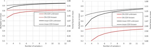
Figure 3. Outcome of equations (1) to (4) for n = 4 and 10 with respect to COV. The multiplier on the mean is the factor $x_k/\mu \left(x\right)$, and the partial factor on mean is the inverse.

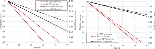
The following observations that can be drawn from Figures 2 and 3:

1. The difference between a characteristic value for a 5% point fractile value and a 5% mean fractile value is rather large and increases with the value of COV.

2. The difference between the characteristic value in the case of known and unknown COV values is relatively large for small sample sizes and increases with the value of COV.

3. For samples sizes less than 10 the multiplier factor decreases rapidly, especially with increasing COV.

There are a number of other equations presented for the evaluation of the characteristic value. As the t-distribution is a bell-shaped distribution that approaches the normal distribution with increasing number of samples, it is considered well suited for properties that are distributed according to distributions resembling the normal distribution. The normal distribution is unbounded, which means it is possible to produce an absurd negative value for positive-valued variables such as undrained shear strength or friction angle when the COV is large, fractile is low, and number of samples is small. However, in the case of Eq. 5 with n = 1, the characteristic value of the mean is only negative when COV > 60%. Hence, Eq. 5 remains reasonably practical for most soil properties with low to medium variability based on the three-tier variability classification scheme shown in Table 1. This scheme has been expanded to classify model uncertainty recently (Phoon and Tang 2019; Tang and Phoon 2021). Equations, covering both general and simplified approaches for evaluation of the characteristic value for properties that are lognormally distributed and have COV ≥ 30%, have been suggested, e.g. Schneider and Schneider (2013).

Table 1. Three-tier classification scheme of soil property variability for reliability calibration (Source: Table 9.7; Phoon and Kulhawy 2008).

Geotechnical parameter	Property variability	COV (%)
Undrained shear strength	Low^a	10–30
	Medium^b	30–50
	High^c	50–70
Effective stress friction angle	Low^a	5–10
	Medium^b	10–15
	High^c	15–20
Horizontal stress coefficient	Low^a	30–50
	Medium^b	50–70
	High^c	70–90

^a Typical of good quality direct lab or field measurements.

^b Typical of indirect correlations with good field data, except for the standard penetration test (SPT).

^c Typical of indirect correlations with SPT field data and with strictly empirical correlations.

In relation to observation (1) above, it might be sometimes difficult to determine whether one should use the 5% fractile for a point value or for the mean. With respect to Equation (1) such consideration is often accounted for by applying a variance reduction factor Γ_S² (Vanmarcke 1977, 2010) to the spatial variability. This requires an estimation of the scale of fluctuation (δ), which is the distance over which soil properties are strongly correlated. Cami et al. (2020) conducted a comprehensive review of spatial variability and tabulated scales of fluctuation for reference. The approximate value for Γ_S² = 1 when the averaging length (L) is shorter than the scale of fluctuation. This is the “local failure” scenario. For the case of averaging length much larger than the scale of fluctuation, the approximate value for Γ_S² = δ/L. Based on the definition of δ, the indicative number of uncorrelated samples in L is n = L/δ. Hence, Γ_S² = 1/n, which is similar to the “mean failure” scenario. It is clear that the contribution from the spatial variability diminishes for the non-local problem. However, for many design situations the value of Γ_S² would lie between the two scenarios. As a refinement, equations have been suggested where the actual zone of influence for the limit state in question is considered. Schneider and Schneider (2013) adopted the following simplification for the variance reduction factor along a prescribed non-critical path, which is that ${\mathrm{\Gamma }}_{\mathrm{S}}^2$ = ${\mathrm{\Gamma }}_x^2{\mathrm{\Gamma }}_y^2{\mathrm{\Gamma }}_z^2$, where ${\mathrm{\Gamma }}_{\mathrm{x}}^2$ and ${\mathrm{\Gamma }}_{\mathrm{y}}^2$ are the variance reduction factors in the two horizontal directions, x and y, and ${\mathrm{\Gamma }}_z^2$ is the variance reduction factor in the vertical direction, z defined by Vanmarcke (1983) and modified Equation (5) to account for the reduction in COV due to spatial averaging: (6) $X_{kmean}=X_{mean}\cdot \left[1-1.645\cdot CO{V}_{inherent,X}\cdot \sqrt{{\mathrm{\Gamma }}_S^2}\right]$(6) In addition, Orr (2015) proposed an equation to cover the extent and quality of investigations, extreme value of the parameter and zone of influence.

It is not always easy to identify the correct failure path/surface in advance. For example, in slope stability analysis there might be a wide range of potential failure paths/surfaces that need to be analysed before the critical path/surface is identified. Some research has been conducted to further refine Equation (6) to account for mean reduction along the critical path. Note that the mean along the critical path is smaller than the mean along a prescribed path/surface shown in Equation (6) (Ching and Phoon 2013a, 2013b; Ching, Phoon, and Kao 2014; Hu and Ching 2015; Ching, Lee, and Phoon 2016; Ching, Hu, and Phoon 2016; Ching, Tong, and Hu 2016; Ching, Phoon, and Pan 2017; Ching, Sung, and Phoon 2017). This is a challenging research question that has not been fully resolved, although some simple solutions for routine structures have been developed recently (Tabarroki et al. 2021). Only the mean value [Equations (3) and (5)] and the point value [Equations (2) and (4)] cases are included in the new EN 1997–1 draft. It will be demonstrated in the next section that these equations can be easily modified to provide significantly better solutions for common/routine geotechnical structures.

With respect to observation (2) it is worthwhile noting that even if the value of COV is assumed based on some general dataset, its value might be large, often even well above 30%. This results in very small characteristic values compared to the mean. For example, for COV = 40% the characteristic value is of the order of 30% of the mean. Applying such an approach, for example to the undrained shear strength of soft clays, would then surely be needed to be balanced with a priori knowledge of the minimum undrained shear strength to avoid physically impossible low values. It is well known that the critical state friction angle and the remoulded undrained shear strength are less uncertain than their peak values and they are arguably reasonable lower bounds. The statistical method has occasionally attracted criticisms that it is not applicable to geotechnical engineering, because it was found to produce results at odds with reality. In the opinion of the authors, there is nothing wrong with statistics. It has been widely adopted in all disciplines. The issue is the adoption of overly simplistic assumptions rather than the generality of the method. In this example, the adoption of a distribution with an appropriate lower bound would address the criticism of an unrealistic fractile value. It is worth pointing out that a simple Johnson family of distributions exist that can cater to both lower and upper bounds (Johnson 1949; Ching and Phoon 2015). The Johnson family is obtained from three closed-form transformations of the normal distributions. The most well-known is the lognormal distribution.

Observation (3) simply suggest that the minimum sample size should be kept close to 10.

3. Considerations beyond statistics

There are several statistical, mechanistic and practical considerations that are relevant to the selection of characteristic values. It is worth demarcating these issues explicitly and describing them individually, before discussing their inter-dependencies.

(1) Value affecting the occurrence of the limit state

The limit state is a question of mechanics, not a question of statistics. For ULS, this requires a knowledge of the critical failure path/surface. The “value affecting the occurrence of the limit state” for ULS can be interpreted as the pertinent average strength value mobilised along the critical failure path/surface. It is important to note that the critical failure path/surface is the solution of a boundary value problem and it can change from one realisation of the random field to the next. It is evident the mobilised value (say strength) along the critical path/surface is not the same as the mobilised value along a prescribed potential path/surface. In limit equilibrium analysis, the critical failure path/surface is defined as the potential path/surface with the lowest factor of safety. A minimisation step is required. For spatially varying soils, it is also important to note that classical solutions for homogeneous soils are not applicable in general. The failure mechanisms in spatially heterogeneous soils can be non-classical.

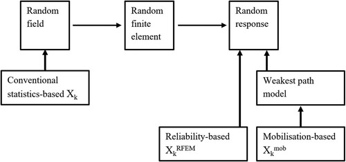
Hicks and Samy (2002) proposed a method of simulating the “effective property” for a spatially heterogeneous soil mass based on the random finite element method (RFEM) (Fenton and Griffiths 2008). The effective property for a particular random field realisation is defined as the homogeneous input property that matches the same performance response as the RFEM. In the context of ULS, the concept of the effective property was also adopted by Ching and Phoon (2013a) and Ching, Sung, and Phoon (2017) to homogenise a soil mass with spatially heterogeneous shear strength. However, they adopted the term “mobilized shear strength” for the effective property. In essence, the mobilised shear strength is the value affecting the occurrence of ULS. Hence, the characteristic value can be taken to be the 5% fractile of the mobilised shear strength, and this particular characteristic value for ULS is called the reliability-based characteristic value (Hicks 2013; Hicks et al. 2019) and is denoted by X_kRFEM in the current paper. X_kRFEM not only addresses the spatial averaging over the influence zone, but it also addresses non-classical mechanisms caused by spatial variability (e.g. seeking out weak zones). The main limitation of X_kRFEM is that it relies on RFEM, so a simple analytical expression similar to Equations (2–6) for X_kRFEM does not exist. For spatially heterogeneous shear strength, this limitation has been overcome by Tabarroki et al. (2021). Tabarroki et al. (2021) calibrated the weakest-path model (WPM) for the mobilised shear strength simulated by 2D RFEM. This WPM is a two-parameter model developed by Ching and Phoon (2013b) and Ching, Sung, and Phoon (2017): one parameter is the variance reduction factor ${\mathrm{\Gamma }}_{\mathrm{S}}^2$ that considers the spatial averaging over the failure zone (influence zone), whereas the other parameter k quantifies the tendency for the failure path to seek out mechanically admissible weak zones. 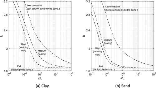The following simple analytical expression for the “mobilisation-based” characteristic value (denoted by X_kmob) is derived from the calibrated WPM: (7) $X_{kmob}=X_{mean}\cdot \left[1-k\cdot CO{V}_{inherent,X}\cdot \sqrt{{\mathrm{\Gamma }}_S^2}\right]$(7) where k is calibrated by RFEM results in Tabarroki et al. (2021). It turns out that the calibrated k depends on two factors: (a) the degree of constraint (low, medium, high, and full) of the failure zone and (b) the normalised scale of fluctuation (δ/L) (δ = the scale of fluctuation and L = length of the classical failure path/surface). For clay with COV_inherent,X = 0.3 for its undrained shear strength (isotropic scales of fluctuation), the variation of the RFEM-calibrated k with respect to δ/L is shown in Figure 4a. For sand with COV_inherent,X = 0.1 for its friction angle (also isotropic scales of fluctuation), the variation of the RFEM-calibrated k with respect to δ/L is shown in Figure 4b. For problems with full constraint (e.g. friction piles in compression, no weak zone seeking), k = 1.645 and Equation (7) reduces to Equation (6). High constraint is exemplified by the active failure of a retaining wall (failure path/surface passes through the toe and is usually close to a straight line), medium constraint by the ultimate failure of a footing (failure path/surface passes through a footing corner), and low constraint by the failure of a soil-cement column in compression (failure path/surface varies relatively free with regard to orientation and location).

Figure 4. Variation of k with respect to δ/L.

Figure 5 illustrates the relation between conventional statistics-based (e.g. Equations 2–5), mobilisation-based (X_kmob in Equation. 7), and reliability-based characteristic values (X_kRFEM). The conventional characteristic value is purely related to the input random field. It is cheap to calculate, but it is not related to the value affecting the occurrence of the limit state at the detailed failure mechanism level. The authors consider the demarcation into “local” and “mean” failure mechanisms to be a gross simplification of the mechanics. The reliability-based characteristic value is an outcome of RFEM, and it is thus related to the occurrence of the limit state at the most detailed failure mechanism level. The mobilisation-based characteristic value approximates the reliability-based characteristic value. It tries to capture sufficient mechanics without incurring the RFEM cost. Equation (7) does not require the engineer to grapple with the choice between “local” and “mean” failure mechanisms. The actual failure mechanism is more likely to fall between these two simplified extremes. The authors submit that Equation (7) it is a significant improvement, because it removes the artificial binary choice between “local” and “mean” failure mechanisms and it correctly addressed the interaction between statistics and mechanics.

Figure 5. Statistics-based, mobilisation-based, and reliability-based characteristic values

(2) 5% fractile value

The need to consider a conservative value implies that the values of interest are not exactly known, due to a number of reasons mentioned above. The key difference between applying judgment and a fractile to determine this conservative value is that the latter is more defensibly linked to measured data and one can handle complex issues beyond the reach of judgment, e.g. multivariate data and mobilised strength along critical failure path/surface. It has been emphasised that fractiles can never be unrealistic if an appropriate probability distribution is adopted (e.g. a distribution bounded from below by the critical state strength).

(3) Cautious estimate

In EN 1997–1 (CEN 2004) a cautious estimate and a 5% fractile value are almost synonymous. (def of cautious). Traditionally, a cautious estimate also includes judgement in relation to how a measured value from a test represents the field conditions. There might be a need to account for time and rate effects or the quality of samples and/or test to the measured values. A fractile value should thus not be taken directly from measured values, rather from values representing the general field conditions. In short, a fractile value should be determined based on correct mechanics and statistics. It is inadequate to consider mechanics or statistics alone – both aspects are not mutually exclusive and interact with each other. Ching and Phoon (2013c) demonstrated that the undrained shear strength can be corrected for test mode, overconsolidation ratio, and strain rate in a statistically consistent way.

(4) Fixed partial factors

Partial factors are customarily regarded as fixed in all current national annexes for EN 1997-1. However, there will be site differences even when a design code is restricted to a country. For example, spatial variability, testing methods, transformation models, etc. can result in different levels of uncertainty (Phoon and Kulhawy 2008) – see Table 1. Phoon (2017) highlighted that “geotechnical design is less amenable to standardisation than structural design and the engineer should be able to exercise his/her discretion to adjust the resistance factor and/or characteristic resistance to suit a particular site and other localised aspects of geotechnical practice”. The issue here is that site-specificity is a core consideration in geotechnical design and construction. Denver and Ovesen (1994) pointed to the number and quality of tests as one aspect of practice that can vary from site to site. However, there are many other site-specific aspects, such as those mentioned above, in addition to the extent of prior knowledge accrued from similar ground conditions and past design and construction experiences with similar structures. At present, there is no consensus on whether it is better to: (1) keep the partial/resistance factor constant while adjusting the characteristic value to suit site conditions, (2) allow the partial/resistance factor to vary with site conditions while keeping the characteristic value fixed at a cautious estimate or particular fractile of the mean value, or (3) allow the partial/resistance factor and the characteristic value to vary. Phoon (2017) pointed out that the second approach has been adopted by Phoon, Kulhawy, and Grigoriu (2003a), Phoon and Kulhawy (2008), the Canadian Highway Bridge Design Code (CAN/CSAS614:2014), and ISO2394:2015 (Phoon et al. 2016). The value of a resistance factor depends on the soil property variability (low, medium, high) in Phoon, Kulhawy, and Grigoriu (2003a) and Phoon and Kulhawy (2008) and the “degree of understanding” (low, typical, high) in CAN/CSAS614:2014. A more detailed discussion is presented in Section 4.1. The practice of using fixed partial factors means one must entertain the use of an adjustable characteristic value to ensure site differences are accounted for in the final design value (characteristic value divided by the partial factor). EN 1997–1 (CEN 2004) adopts this practice. It is not surprising that the characteristic value has become a major source of controversy and difficulty in the implementation of Eurocode 7. An important related question is what issues are amenable to engineering judgment and what issues are more effectively resolved using data and data-driven methods. The reliability calibration of partial factors is an example of relieving the engineer from making risk-informed decisions using engineering judgment alone without any formal aid. Reasoning in the face of uncertainty is not intuitive.

(5) Sensitivity of limit state to inputs

Phoon (2017) further noted that a large uncertainty at the input level does not necessarily translate into a large uncertainty in the response – this is related to how sensitive is the limit state to a particular input parameter. The discussion on how to select a conservative value thus far is restricted to the input stage, although one may argue that a larger conservative margin is justified for more sensitive parameters. On the other hand, it is possible to argue that EN 1997–1 (CEN 2004) does not subscribe to the notion of maintaining uniform reliability (this is the goal of reliability-based design) and it is acceptable to produce designs of widely differing implied levels of reliability. However, the authors do not think this argument can be carried to the extreme – not maintaining a uniform reliability does not mean engineers are willing to accept widely differing levels of conservatism. One way of looking at “acceptable conservatism” is to look at the range of reliability implied by existing designs. Phoon, Kulhawy, and Grigoriu (1995, 2003a) have shown that many foundations designed using the working stress method carry implied reliability levels spanning two orders of probabilities of failure. To keep within this range (2 orders of magnitude), engineers have applied judgment to adjust input parameters according to sensitivity as well. From Figure 5, it can be seen that the current statistics-based equations do not consider this sensitivity aspect. The reliability-based characteristic value considers sensitivity exactly through the use of RFEM. The mobilisation-based characteristic value considers sensitivity approximately because it is calibrated from RFEM.

The key point in the above discussion is that the selection of a characteristic value in its current form must necessarily involve a proper appreciation of mechanics and statistics and their interaction, as well as some degree of judgment, because there are issues beyond broad qualitative appreciation of mechanistic considerations and statistics. For example, the sensitivity of inputs to limit state requires a knowledge of the output from a mechanistic analysis. However, the conventional characteristic value is an input to this analysis – it is not the “value affecting the occurrence of the limit state”. This value can be the spatial average along a critical slip surface which is an output of say a limit equilibrium analysis. The crucial difference between a critical slip surface and a prescribed slip surface is not well appreciated. This is the fundamental gap that judgment is asked to bridge (Figure 5). This gap is not evident for an ideal case of a homogeneous soil mass. It may not be surprising that engineers find it difficult to estimate this characteristic value, because the concept is loaded with too many issues. One can imagine the difficulty of visualising even remotely the response of a complex 3D soil-structure problem that is outside one’s experience base even qualitatively. On the other hand, the partial factor approach (which is associated with the concept of the characteristic value) appears to be applicable only to familiar Category 2 problems – not unusual and complex problems. Nonetheless, even for familiar problems such as slopes, foundations and retaining structures, judgment is unlikely to be effective to consider inter-dependencies between these issues as they are complex. They can involve physical and/or statistical complexity. For example, the failure path/surface (mechanism) for spatially variable soil is not the same as for homogeneous soil. How does one visualise the failure mechanisms in spatially heterogeneous soils for all plausible or the most critical random field realizations consistent with limited borehole data? The correlations between multiple input parameters are difficult to untangle using judgment alone. It is known that prescribing a 5% fractile for all input parameters is excessively conservative unless all parameters are correlated (Ching et al. 2020b). An SLS problem involving multiple input parameters is presented in Section 4.2 to illustrate the difficulty of extending the current understanding of a characteristic value in the context of multiple input parameters. Note that almost all geotechnical problems are governed by multiple input parameters – this is the norm, not an exception.

4. Use of characteristic values for different limit states and analysis

4.1. Characteristic values for ULS analysis

In ULS design the use of a cautious estimate can be seen as a continuation of traditional (sound) design procedures. However, the variation of material properties is in many cases a substantial source of uncertainty in geotechnical design. In EN 1997–1 (CEN 2004) a single constant partial factor is applied to the material property. In some situations, for example in ULS designs where there are only permanent loads and the partial load factor is unity, this is the only source of safety applied in the calculation, apart from the safety provided through the selection of the cautious characteristic material property value. As mentioned above, this places a substantial demand on the selection of the characteristic values as it should account for all the site and investigation specific variation of uncertainty of the material property and a broad appreciation of the soil-structure interaction mechanism (“value affecting the occurrence of the limit state”). It can be debated if subjectively chosen best estimate values or a simple statistical procedure can solely account for this uncertainty. Alternatively, one could apply a partial factor that would depend on the degree of uncertainty. This follows one of the original principles from which the partial safety factor method was first proposed by Hansen (1965); a higher safety margin is applied where/when there is higher uncertainty.

This kind of approach was introduced in the 1995 reliability-based design guidelines for transmission line structure foundations (Phoon, Kulhawy, and Grigoriu 1995, 2003a), the 2014 Canadian Highway Bridge Design Code (CAN/CSAS614:2014), and ISO2394:2015 (Phoon et al. 2016). The resistance factors in CAN/CSAS614:2014 have been calibrated based on reliability to reflect the degree of understanding in the following three-level or three-tier system:

• High understanding: Extensive project-specific investigation procedures and (or) knowledge are combined with prediction models of demonstrated quality to achieve a high level of confidence with performance predictions;

• Typical understanding: Typical project-specific investigation procedures and (or) knowledge are combined with conventional prediction models to achieve a typical level of confidence with performance predictions;

• Low understanding: Limited representative information (e.g. previous experience, extrapolation from nearby and (or) similar sites, etc.) are combined with conventional prediction models to achieve a lower level of confidence with performance predictions.

For example, for the analysis of the bearing capacity of shallow foundations the resistance factors are 0.45, 0.50 and 0.60 for low, typical, and high degree of understanding, as shwon in Table 2. Länsivaara and Poutanen (2014) also suggested a similar approach in which the partial factors of safety for soil strength are related to the coefficient of variation. Phoon, Kulhawy, and Grigoriu (1995, 2003a) have shown that it is possible to achieve a significantly improved uniformity in the reliability of designs when they are based on resistance factors calibrated to a three-tier classification scheme for the coefficient of variation (see Table 1). This reliability calibration exercise can be expanded to include a new three-tier classification for model uncertainty (Phoon and Tang 2019; Tang and Phoon 2021). The degree of improvement can be objectively benchmarked against the range of reliability indices produced by working stress designs based on a single factor of safety (conceptually the same as a single resistance factor). Phoon, Kulhawy, and Grigoriu (1995, 2003a) showed that the probabilities of failure for allowable stress design typically vary across two orders of magnitude for a variety of foundation designs for transmission line structures. The key point is that it is possible to account for uncertainty in an objective way based on measured data without having a precise estimate of the coefficient of the variation. The need to strengthen the link between decisions and data has become more pressing with the rapid growth in digital technologies (Phoon 2020).

Table 2. Geotechnical resistance factors for the ultimate limit state (ULS) and serviceability limit state (SLS) appearing in Table 6.2 of the 2014 Canadian Highway Bridge Design Code (CHBDC) (CAN/CSAS614:2014). Numbers are for illustration only – the 2014 CHBDC must be consulted for the actual factors (Source: Table 4; Fenton et al. 2016).

Application	Limit State	Test Method/Model	Degree of understanding
			Low	Typical	High
Shallow foundations	Bearing, ${\phi }_{gu}$	Analysis	0.45	0.50	0.60
		Scale model test	0.50	0.55	0.65
	Sliding, ${\phi }_{gu}$ Frictional	Analysis	0.70	0.80	0.90
		Scale model test	0.75	0.85	0.95
	Sliding, ${\phi }_{gu}$ Cohesive	Analysis	0.55	0.60	0.65
		Scale model test	0.60	0.65	0.70
	Passive resistance, ${\phi }_{gu}$	Analysis	0.40	0.50	0.55
	Settlement or lateral movement, ${\phi }_{gs}$	Analysis	0.70	0.80	0.90
		Scale model test	0.80	0.90	1.00
Deep foundations	Compression, ${\phi }_{gu}$	Static analysis	0.35	0.40	0.45
		Static test	0.50	0.60	0.70
		Dynamic analysis	0.35	0.40	0.45
		Dynamic test	0.45	0.50	0.55
	Tension, ${\phi }_{gu}$	Static analysis	0.20	0.30	0.40
		Static test	0.40	0.50	0.60
	Lateral, ${\phi }_{gu}$	Static analysis	0.45	0.50	0.55
		Static test	0.45	0.50	0.55
	Settlement or lateral deflection, ${\phi }_{gs}$	Static analysis	0.70	0.80	0.90
		Static test	0.80	0.90	1.00
Ground Anchors	Pull-out, ${\phi }_{gu}$	Analysis	0.35	0.40	0.50
		Test	0.55	0.60	0.65
Internal MSE reinforcement	Rupture, ${\phi }_{gu}$	Analysis	0.75	0.80	0.85
		Test	0.85	0.90	0.95
	Pull-out, ${\phi }_{gu}$	Analysis	0.35	0.40	0.50
		Test	0.55	0.60	0.65
Retaining systems	Bearing, ${\phi }_{gu}$	Analysis	0.45	0.50	0.60
	Overturning, ${\phi }_{gu}$	Analysis	0.45	0.50	0.55
	Base sliding, ${\phi }_{gu}$	Analysis	0.70	0.80	0.90
	Facing interface sliding, ${\phi }_{gu}$	Test	0.75	0.85	0.95
	Connections, ${\phi }_{gu}$	Test	0.65	0.70	0.75
	Settlement, ${\phi }_{gs}$	Analysis	0.70	0.80	0.90
	Deflection/tilt, ${\phi }_{gs}$	Analysis	0.70	0.80	0.90
Embankments (fill)	Bearing, ${\phi }_{gu}$	Analysis	0.45	0.50	0.60
	Sliding, ${\phi }_{gu}$	Analysis	0.70	0.80	0.90
	Global stability-temporary, ${\phi }_{gu}$	Analysis	0.70	0.75	0.80
	Global stability-permanent, ${\phi }_{gu}$	Analysis	0.60	0.65	0.70
	Settlement, ${\phi }_{gs}$	Analysis	0.70	0.80	0.90
		Test	0.80	0.90	1.00

4.2. Characteristic values for SLS analyses

4.2.1. Selection of characteristic values for SLS analyses

While EN 1990 (CEN 2002) generally recommends the use of mean values as characteristic values for stiffness parameters, EN 1997–1 indicates that cautious estimates should be used as characteristic values also in SLS. In the 2021 draft version of prEN 1997–1 (CEN 2020) the design values are determined using the same principles for ULS and SLS analyses, applying partial factors which, for SLS analyses, the recommended values are 1.0, to representative values, which in turn are based either on cautious estimates or statistics. The underlying logic seems to be that for a mean value, or more precisely, for the median value, the limit state would be exceeded with a 50% probability. This though depends on the definition of the allowable deformations as well as on the loads that are used. A safety margin could also be achieved by introducing safety to the calculated settlements. For example, in the 2014 Canadian Highway Bridge design code discussed above, resistance factors are also introduced for SLS calculation. The Canadian Highway Bridge design code uses the term “resistance factor” for both ULS and SLS, although it is more appropriate to use the term “deformation factor” for SLS. These factors also reflect the degree of understanding and are for example for the settlement analysis of a shallow foundation 0.70, 0.80 and 0.90 for low, typical, and high degree of understanding as shown in Table 2. Deformation factors for SLS have been recommended as early as 1995 (Phoon, Kulhawy, and Grigoriu 1995, 2003a). An example is shown in Table 3 for footings subjected to uplift.

Table 3. Undrained uplift resistance/deformation factors for LRFD (Phoon, Kulhawy, and Grigoriu 2003a).

			Ψu
Depth/Width	Width (m)	COV of K (%)	Resistance factor (ULS)	Deformation factor (SLS)
1–2	1 – 2	30–50	0.45	0.69
		50–70	0.43	0.66
		70–90	0.41	0.63
	2 – 3	30–50	0.42	0.63
		50–70	0.40	0.60
		70–90	0.38	0.58
2–3	1 – 2	30–50	0.41	0.62
		50–70	0.38	0.58
		70–90	0.36	0.55
	2 – 3	30–50	0.39	0.58
		50–70	0.36	0.54
		70–90	0.34	0.51

Note: K = operative horizontal stress coefficient; target reliability index = 3.2 for resistance factors (ULS) and 2.6 for deformation factors (SLS)

A noteworthy point here is that although the reliability index for SLS is lower than that for ULS, because the consequences of failure are arguably less severe (as far as protection of lives are concerned), the reliability index for SLS is not zero which corresponds to 50% probability of exceeding the SLS. This is why for SLS calculations prEN 1997–1 (CEN 2020) requires that design material parameter values are used that are characteristic values, i.e. a cautious estimate or 5% a fractile value, divided by a partial factor equal to unity to provide the required reliability against the allowable deformations being exceeded. For the simple case of two independent lognormal random variables, it can be shown theoretically that the partial factor corresponding to a 5% fractile value is exp[(1.645-0.75×β)×COV], in which β is the reliability and COV is the coefficient of variation (Ravindra and Galambos 1978). A partial factor of unity implies a reliability index of 2.2. Phoon, Kulhawy, and Grigoriu (1995, 2003a) calibrated an annual reliability index of 3.2 and 2.6 for ULS and SLS respectively. With reference to Table C2 of EN1990 (CEN 2002), the annual, i.e. 1 year, target reliability indexes for ULS and SLS are 4.7 and 2.9, respectively, while the 50 year target reliability indexes are 3.8 and 1.5.

One shortcoming of the argument for using 5% fractile values for SLS is that uncertainties related to the SLS calculation output are not just related to the choice of soil parameters. There are certainly many other uncertainties involved, such as those present in the estimation of loads or in the choice of calculation model. In an extensive survey of load test databases, Tang and Phoon (2021) concluded that the model factors for many settlement calculations methods are of high dispersion (coefficient of variation larger than 0.6). It is not consistent nor justified to try to cover all this in the evaluation of characteristic soil parameters. Additionally, for settlement analysis, it is not necessarily the maximum total settlement that is the governing limit state; differential settlement is often more critical. It is thus not always the lower fractile value that is decisive, but rather a combination of lower and upper fractile values. However, to search for the worst combination of these could be very laborious at this point.

When the output of a geotechnical calculation is governed by multiple parameters, the determination of a cautious estimate or fractile value gets more complicated. The parameters might well be correlated, and an independent evaluation of the characteristic value is no longer possible. The examples that are usually given, for example in relation to EN 1997–1 (CEN 2004), are for simple single parameters such as the undrained shear strength s_u, Young’s modulus E or compression index C_c. When introducing equations to determine characteristic values it is thus often left to the engineer to figure out how to apply them for more complicated parameter sets.

4.2.2. Settlement analysis example

To address the problem of how to select the characteristic values for SLS analyses in the presence of multiple input parameters, a basic settlement analysis example is considered, utilising the Janbu constrained modulus M, defined as; (8) $M=m\cdot {\sigma }_a\cdot {\left({\displaystyle \frac{\sigma {}^{\mathrm{\prime }}}{{\sigma }_a}}\right)}^{1-a}$(8) Where m is the modulus number (dimensionless), a the stress exponent (dimensionless), σ_a reference stress (= 100 kPa) and σ’ the effective vertical stress. The task is to calculate the total settlement for an 8.5m thick, soft clay layer under a load of 30 kPa. Above the soft clay layer, a 1.5 m thick stiff crust, referred to in Figure 6 as Dry crust, can be found. As the deformation of the crust is minimal in comparison to the soft clay layer, it is not considered here. To evaluate the deformation properties of the soft clay, four oedometer tests have been carried out, whose results are presented in Table 4, where w is the water content and σ'_cv is the preconsolidation pressure. For the overconsolidated region a constant constrained modulus M_OC is applied, while for the normally consolidated region the modulus number m and stress exponent a are applied using Equation (8). In the evaluation of the results, engineering judgment has been used and effects of strain rate and sample quality have been assessed. As the qualities of the soft clay layer change with depth, it was decided to divide the layer into four sub-layers, Clay 1–4, according to the oedometer results. The division of layer, in situ effective vertical stress, preconsolidation profile, and final stress state is presented in Figure 6. For Clay 3 and Clay 4 layers where the preconsolidation pressure is changing with depth, the modulus number in the calculation is modified with respect to the preconsolidation pressure according to Länsivaara (2000, 2012).

Figure 6. In situ effective vertical stress (solid line), preconsolidation profile (dashed line), and final stress state (dotted line) for the settlement example. The square markers indicate the preconsolidation pressure values from the oedometer tests. The groundwater table at 1.5 m depth is indicated by a dashed dotted line.

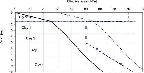
Table 4. Water content and the deformation properties obtained from oedometer tests.

Depth [m]	w [%]	σ’cv [kPa]	MOC [kPa]	m	a
2.5	90.8	50	1400	5.5	−1.1
4.2	118.1	50	1100	4.6	−1.2
6.2	116.8	58	1350	3.7	−1.5
8.7	85.9	75	2000	3.5	−1.35

4.2.3. Settlement analysis using simple statistical characteristic values

In the first set of calculations the characteristic values are calculated as the 5% fractile of the mean assuming that the COV is known, i.e. applying Equation (5). As there are 4 oedometer test results, but the clay layer is also divided into 4 sublayers, it is not obvious if the sample number n should be chosen as 1 or 4. Looking at the trend in the preconsolidation pressure, one may also argue that there are 2 sublayers with similar characteristics. Neither is it obvious regarding the 5% of which parameter or parameters should be chosen to calculate the characteristic settlement. To study the influence of both, the calculations are performed using the combinations presented in Table 5.

Table 5. Combinations for simple statistical characteristic value calculations.

Set of characteristic values	n = 1	n = 4
Best estimate values, i.e. values presented in Table 4.	(X)	(X)
5% mean values for M and a		X
5% mean values for M and m		X
5% mean values for M, m, and a		X
5% mean values for σ’cv	X	X
5% mean values for σ’cv, M and m	X	X
5% mean values for σ’cv, M, m and a		X

In the calculations where a fractile value is applied to the preconsolidation pressure, the minimum value of the preconsolidation pressure in the settlement calculation is the in situ effective vertical stress. For simplicity, it is assumed that the COV values are the same for all parameters. If the constrained modulus M is the only parameter defined at its characteristic value (M_OC and m in the calculation), the ratio of the characteristic settlement to the best estimate settlement can be calculated as the inverse of the multiplier for the mean in Equation (4). This can be expressed by Equation (9). (9) ${\displaystyle \frac{settlemen{t}_{kmodulus}}{settlemen{t}_{bestestimate}}={\displaystyle \frac{1}{\left[1-1.645\cdot CO{V}_X\cdot \sqrt{{\displaystyle \frac{1}{n}}}\right]}}}$(9) The results of the calculation for COV lying between 0 and 30% are presented in Figure 7 as calculated characteristic settlement/best estimate settlement, where best estimate settlement refers to calculation with the best estimate values in Table 4. In Figure 7a) the influence of number of samples is shown. In Figure 7b) all the different combinations of characteristic values are shown for n = 4.

Figure 7. Influence of number of samples a) and comparison of different sets of characteristic values for n = 4 b) to the ratio between characteristic and best estimate settlement.

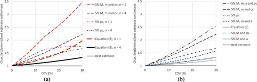
As can be seen from Figure 7a), the choice of n = 1 increases the settlement drastically. However, the authors believe that, although the 4 oedometer tests are conducted in different layers, as they represent the same clay deposit, the number of samples should be taken as four. It can further be seen from Figure 7a) that taking the 5% fractile of the preconsolidation pressure alone, will only have an effect for a certain range of COV values. For the case of n = 1, the characteristic settlement will not increase after around COV = 16% as the reduction of the preconsolidation pressure is limited to the in situ effective vertical stress.

The results in Figure 7b) show a wide scatter for the results with different combinations of characteristic values. It is not obvious which should be chosen but some considerations can be given. Regarding the stress exponent a in Equation (8), there certainly is uncertainty also regarding its determination, related e.g. to the sample quality. However, its value is much related to the soil type. For non-sensitive clays, it is often close to zero, giving then identical behaviour to the compression index method, for sands it is close to 0.5 and the constant constrained modulus M used in the overconsolidated region corresponds to a =1. As one would not normally consider its variation when using the compression index methods, nor when using a constant constrained modulus, the authors suggest that it should be fixed. In practice, this means, that the fractile is determined for the constrained modulus M itself, not for the constituent variables used to model it.

As can be seen from Figure 7 b), the curves for Equation (9) and for taken 5% mean fractile for M_OC and m coincide. For situations where the settlement only depends on the stiffness of the soil and not on the preconsolidation pressure, the situation is relatively simple. This could be e.g. sands or overconsolidated clays. One could then apply either Equation (5) to the stiffness parameters or Equation (9) to the calculated best estimate settlement. The geotechnical resistance factors (equal to deformation factors) corresponding to high, typical, and low degree of understanding are 0.90, 0.80 and 0.70. The inverse of Equation (9) for COV values 10, 20, 30, and 40% are 0.92, 0.84, 0.75, 0.67, i.e. such an approach would be in line with the Canadian Highway Bridge Design Code (CHBDC).

In this example, the preconsolidation pressure is the dominant factor. This is typical for lightly overconsolidated clays where the applied load increases the stresses beyond the preconsolidation pressure. However, as a priori knowledge is used restricting the value of the preconsolidation pressure not to be lower than the effective vertical in-situ stress, its influence is reduced even for n = 4 for COV values beyond 25%. If one adopts a 5% mean fractile value for all the parameters, the calculated settlement for COV = 30% is more than 2.5 times higher than the best estimate value, corresponding to a deformation factor of less than 0.4. However, the influence is strongly dependent on the relation of the overburden stress to the preconsolidation pressure. With increasing overconsolidation ratio, the ratio of the characteristic settlement to the best estimate settlement of 2.5 for COV = 30% decreases towards 1.3. In the authors’ opinion, this emphasises the importance of always carrying out best estimate and sensitivity analyses. The question remains, which characteristic settlement one should use. In all likelihood, this question cannot be answered if Eurocode 7 remains non-probabilistic, because the goal of selecting characteristic values and partial factors to achieve a uniform reliability level is only meaningful within a reliability-based design framework, simplified or otherwise. It is worth pointing out that a non-probabilistic approach offers less data-informed support for decision making, notwithstanding other considerations debated elsewhere (Phoon 2017). For example, it is not possible to consider correlations between different soil parameters in a non-probabilistic framework. Correlations do exist empirically and are widely used in practice in the form of transformation models. As an example, Janbu proposed a correlation between the modulus number m and the water content in the form m = 700/w% ±30%, for stress exponent a = 0 (Janbu 1995). Di Buò et al. (2018) suggested that the constant constrained modulus for the overconsolidated region can be evaluated based on the preconsolidation pressure given by M = σ’_cv/0.03. They are not theoretical abstractions invented to make a case for reliability analysis but are critical to generalising the concept of the characteristic value derived from a single to multiple parameters (Ching et al. 2020b). A non-probabilistic framework cannot address the more critical limit state of differential settlement that can only arise from spatially varying soils.

4.2.4. Settlement analysis using reliability-based characteristic values

Hicks (2013) and Hicks and Nuttall (2012) proposed that characteristic values should be selected to give a failure probability of 5% with respect to the system response. Hicks (2013) and Hicks and Nuttall (2012) denote such characteristic values as the reliability-based characteristic values (X_kRBD). The corresponding settlement is referred to as the reliability-based characteristic settlement (settlement_kRBD). It is clear that settlement_kRBD is the 1–5% = 95% fractile value of the settlement, which can be determined by Monte Carlo simulation (MCS).

In order to perform the reliability-based characteristic settlement calculations some further assumptions are needed. One needs to consider the correlations between the parameters, both the spatial (auto-correlation) and the physical (cross-correlation), as well as assume distributions for the parameters. In the following the cross-correlations for parameters σ’_cv, M, and m are considered, while the exponential a is assumed to be fixed.

There are four clay layers, and each layer has its own (σ’_cv, M, m). As a result, there are in total 12 parameters. The spatial correlation among the four clay layers is considered by assuming the single exponential auto-correlation model: (10) $R_z=\left(\begin{array}{cccc}1& e^{-2\left|z_1-z_2\right|/SOF}& e^{-2\left|z_1-z_3\right|/SOF}& e^{-2\left|z_1-z_4\right|/SOF}\\ & 1& e^{-2\left|z_2-z_3\right|/SOF}& e^{-2\left|z_2-z_4\right|/SOF}\\ & & 1& e^{-2\left|z_3-z_4\right|/SOF}\\ SYM& & & 1\end{array}\right)$(10) where (z₁, z₂, z₃, z₄) are the mid depths of the four layers, and SOF is the assumed vertical scale of fluctuation. The cross-correlation among the four parameters is considered as follows: (11) $R_{cross}=\left(\begin{array}{ccc}1& \rho \left({{\sigma }^{\mathrm{\prime }}}_{cv},M\right)& \rho \left({{\sigma }^{\mathrm{\prime }}}_{cv},m\right)\\ & 1& \rho \left(M,m\right)\\ SYM& & 1\end{array}\right)$(11) The correlation matrix R for the 12 parameters is equal to the Kronecker-product between R_z and R_cross: (12) $R=R_{cross}\otimes R_z$(12) With the marginal distributions of (σ’_cv, M, m) and the correlation matrix R, the translation method (Johnson 1949; Li et al. 2012) is adopted to simulate N = 10⁴ samples of (σ’_cv, M, m). These samples are used to compute N settlement samples, and settlement_kRBD is therefore the 1–5% = 95% sample fractile value.

To the authors’ knowledge there are no data about the correlation between (σ’_cv, M, m). As the preconsolidation pressure of soft clays for good quality samples is generally reached with a compression of 3–4 %, one could argue that there is a strong positive correlation between σ’_cv and M. On the other hand, when fitting the parameters to the observed behaviour from an oedometer test, an increased σ’_cv value needs to be compensated by reducing the m value. To study the influence of cross-correlation two different assumptions are made. First, a strong positive correlation of 0.8 is assumed between σ’_cv and M, whereas a weak positive correlation of 0.3 is assumed between σ’_cv and m and between M and m. A second calculation is made using a negative correlation of −0.5 between σ’_cv and m and σ’_cv and M, while no correlation is assumed between M and m. For both cross-correlation scenarios, calculations are performed for the cases of: (a) number of samples n = 4 and SOF as a large number (10000) and (b) n = 1 and SOF = 1. The results of these calculations are presented in Figure 8a).

Figure 8. Reliability based characteristic settlement calculations. The influence of positive vs. negative correlation a), the influence of normal vs. log normal distributions b), comparison of RBD vs. ERD characteristic settlement calculations c) and comparison of simple static and RBD/ERD characteristic settlement calculations for n = 4.

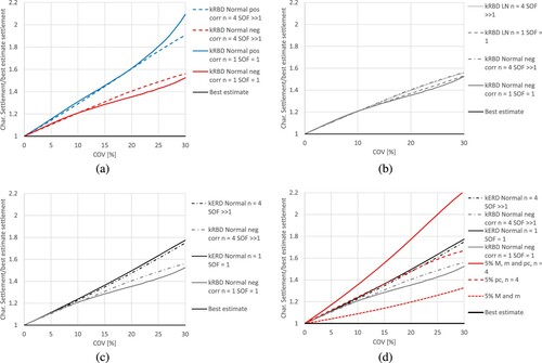
As can be seen, the biggest influence is caused by the assumption of either positive or negative correlation. As the major part of the settlement comes from the normally consolidated region, the assumed cross-correlation between σ’_cv and m is the most important. Although the are no reported data on the cross-correlation between these parameters, the authors believe that the cross-correlation between σ’_cv and m is likely to be negative, based on the earlier consideration about parameter determination. The following calculations are thus carried out using only the negative cross-correlation scenario.

Next a comparison between normal and log normal distributions for the parameters is made. For this comparison as well, the calculations for each distribution are performed for the cases of: (a) number of samples n = 4 and SOF as a large number (10000) and (b) n = 1 and SOF = 1. The results are presented in Figure 8b). As can be seen, the differences between results from assuming normal or log normal distributions are, even surprisingly, small. Therefore, the following calculations will be carried out using the normal distribution only for consistent comparison with the simple characteristic value calculations.

In practice, the goal is to find the appropriate characteristic values or fractile inputs (i.e. X_kRBD) such that the desired fractile response (i.e. settlement_kRBD) is achieved. However, the above MCS procedure can only evaluate settlement_kRBD. It cannot determine X_kRBD. This is a more complicated inverse problem. Recently, Ching et al. (2020b) proposed an approximate method of finding X_kRBD to achieve any desired fractile settlement (settlement_kRBD). In this method, the appropriate characteristic values are defined as the η fractiles of the inputs (X). Note that η is usually not 5%, but it can be calculated using the concept of the effective random dimension (ERD), which is defined as the effective number of independent standard random variables that affects the response (Ching, Phoon, and Yang 2015). ERD can be computed based on the R matrix in Eq. (11(11) $R_{cross}=\left(\begin{array}{ccc}1& \rho \left({{\sigma }^{\mathrm{\prime }}}_{cv},M\right)& \rho \left({{\sigma }^{\mathrm{\prime }}}_{cv},m\right)\\ & 1& \rho \left(M,m\right)\\ SYM& & 1\end{array}\right)$(11) ) and the sensitivity of the response to the inputs. If ERD = 1, η is exactly 5%, if ERD > 1, η is greater than 5%. In general, η can be computed (Ching, Phoon, and Yang 2015) as: (13) $\eta =\mathrm{\Phi }\left[{\mathrm{\Phi }}^{-1}\left(0.05\right)/ER{D}^{0.5}\right]$(13) where Φ is the cumulative distribution function for a standard normal distribution.

For the scenario of negative correlation, ERD is about 1.34 (i.e. there are only about 1.34 effective independent standard normal inputs, although there are apparently 3 input parameters). The η value corresponding to the computed ERD is about 0.077. Therefore, the appropriate characteristic values (denoted by X_kERD) should be calculated using the 7.7% fractiles of the means of X’s: (σ’_cv, M, m), rather than 5% fractiles of the means. The “mean” is assumed to be more appropriate than the “local” mechanism scenario. While the “mean” mechanism is likely to be appropriate under full mobilisation in ULS, it is uncertain if it is equally appropriate under more restricted mobilisation in SLS. This example illustrates the difficulty of making a choice between Equation (4) and (5) when only two options are available. These X_kERD values can be used to compute the characteristic settlement, denoted by settlement_kERD. A comparison of RBD and ERD characteristic value settlements are presented in Figure 8c). As can be seen, the settlement_kERD is reasonably close to settlement_kRBD, and thus X_kERD is deemed to be a reasonable approximation of X_kRBD. It can be noted that ERD gives results on the safe side and that the difference from the RBD results gets smaller as n increases.

In Figure 8d) a final comparison between some of the results from the simple, RBD and ERD calculations are presented. The most important conclusions from this example are;

• Taking a 5% fractile of the mean of all considered parameters (σ’_cv, M, m) leads to overly conservative results, while the correct characteristic values for this example should rather be taken as 7.7% fractiles of the mean.

• Taking a 5% fractile independently for the preconsolidation pressure (σ’_cv) and the constrained modulus (M and m) and using the maximum settlement value as the characteristic value seems to give reasonable results for this example.

• The ERD method produces reasonable approximations for the full RBD.

The complexity of the example arises to a large extent from the low overconsolidation ratio, since deformations occur in both the OC and NC regions, and the difference in the soil stiffness is significant between the two regions. As discussed previously, for simple cases where the settlement is not dependent on the preconsolidation pressure, a simple evaluation could be obtained using Equation (9). This was further verified with RBD and ERD analyses, which for n = 4 and SOF >>1 gave exactly the same result as Equation (9).

One may argue that it is difficult to know what is the correct COV value to use, as it may not be possible to determine it statistically from limited data. It is though possible to use a priori knowledge of the test methods and the quality of the obtained parameters. It is also possible to combine large generic data with limited site-specific data using Bayesian machine learning to obtain a more precise estimate of the COV of the parameters (Phoon 2020). If the oedometer tests have been performed on high quality samples meeting the sample quality criteria (Lunne, Berre, and Strandvik 1997), and consideration of strain rate effects are made, as well as after carrying out careful assessment of other factors such as loads, possible fluctuation of groundwater, etc., it might be justified to use a low COV of the order of 10%. On the other hand, poor sample quality generally causes conservative settlement predictions. It is also important to consider the consequence of exceeding the allowable settlement. If the example represents the construction of a local road, the consequence would not be as severe as in a settlement analysis of, for example, a brick-built house. Judgment is thus stretched in the determination of the parameters, in the evaluation of other calculation inputs and in the evaluation of calculated results. This might partly be based on characteristic value calculations as in the previous example. It is important to note that such calculations do not even attempt to cover all the uncertainties involved in the problem in hand. These need to be considered by other means. A simple and straightforward way to do this would be to use deformation factors, as in Table 2, based on degree of understanding for the whole analysis and multiply these with some consequence factors If the deformation factors are multipliers for the calculated best estimate settlement, such an approach could be as shown in Table 6. If such an approach were adopted it would be advisable to scale the deformation factors in Table 2 with the aid of a comprehensive RBD/ERD analysis.

Table 6. Example of empirical deformation factors (herein defined as multipliers applied to best estimate settlement) depending on the level of understanding and consequence of exceeding the serviceability limit state.

			Consequence
			Low	Normal	High
			1	1.1	1.2
Level of understanding	High	1.1	1.1	1.21	1.32
	Normal	1.3	1.3	1.43	1.56
	Low	1.5	1.5	1.65	1.8

4.3. Characteristic values for FEM analysis

When using the finite element method, the problem of defining characteristic values is perhaps even more complicated than discussed above for general SLS. More and more complicated material models are used in engineering practice. It is not unusual to use soil models having more than ten parameters. These parameters are often correlated so that the selection of one parameter influences the values of some of the other parameters. The performance of such models reflects the combined effect of its parameters, for example stiffness properties can have a considerable influence on the resulting strength and strength properties can have a considerable influence on the resulting stiffness. Applying a 5% fractile to all input parameters simultaneously could be excessively conservative and might lead to unusually large and uneconomical designs. In addition, most of them would rather present speculative values than true 5% fractiles as the COV of many of the parameters would not be known.

As discussed in the previous section, Ching et al. (2020b) studied the determination of the characteristic values in the case of multiple correlated parameters. They showed that if a 5% fractile is applied independently to all correlated parameters, the resulting probability of a worse value governing the occurrence of the limit state can be highly variable, beyond the two orders of magnitude implied in working stress designs. Such an interpretation of the characteristic value, referred to as ITP1 (Interpretation 1) by Ching et al. (2020b), corresponds to the curve with 5% fractile values for M, m a and σ_cv’ in Figure 7b), giving also very conservative results. Ching et al. (2020b) further concluded that Interpretation 2 (ITP2) lacks the problems of ITP1. In the previous example, ITP2 corresponds to the RBD method and, as a simplified version, to the ERD calculations, where a 5% fractile is applied to the output (settlement in the previous example). Note that using a 5% fractile with unit partial factor in an SLS design is equivalent to a reliability index of 2.2 based on the assumptions adopted by Ravindra and Galambos (1978). This is the average of the annual target reliability index (2.9) and 50-year lifetime target reliability index (1.5) for SLS in Table C2 of EN1990. The authors believe that the practical question of how to calculate the fractile for the inputs of any material model to achieve a 5% exceedance probability of SLS can be based on the quantile value method (QVM) (Ching and Phoon 2011) and the concept of an effective random dimension (ERD) (Ching, Phoon, and Yang 2015). No probabilistic analysis is needed, and it may offer a reasonable solution to the problem of selecting multiple characteristic values from correlated inputs as shown in Figure 8. The authors agree that the naïve interpretation of applying a 5% fractile to all inputs (ITP1) is not reasonable.

The authors believe that the simplified QVM-ERD method or the approximate ITP2 method has the potential to be applied in routine practice. Meanwhile, more guidance for the application of characteristic values in FEM is needed. When selecting the parameters of a more complicated soil model, it is a common procedure to simulate laboratory tests to determine/verify the parameters. In addition, calibration tests may be carried out on some structures. There may not be sufficient data about particular parameters to enable fractiles of the best estimate parameters to be selected. Instead, an approach applying deformation factors as in Table 6 could be applied in FEM based SLS analysis. It should be remembered that the difference between the results of analyses due to using different models, say between a linearly elastic-perfectly plastic model and an advanced visco-plastic hardening model, might be more significant than the difference due to the variation of the parameters. Such differences could be included in the level of understanding as in Table 6. At present, the model uncertainties associated with calculation models for foundation capacity and settlement are well studied (Tang and Phoon 2021), but the same cannot be said for different constitutive models in FEM.

Another important issue not well highlighted in the literature is the importance of spatial variability and the necessity of using FEM to solve soil-structure interaction problems in spatially variable soils. Analytical solutions are only possible for homogeneous soils. Note that spatially variable soils are a more realistic representation of “ground truths”. It is not possible to simplify a spatially variable soil mass as an equivalent homogeneous soil mass by simple spatial averaging, because the failure mechanism is different (Ching and Phoon 2013a, 2013b; Ching, Phoon, and Kao 2014; Hu and Ching 2015; Ching, Lee, and Phoon 2016; Ching, Hu, and Phoon 2016; Ching, Tong, and Hu 2016; Ching, Phoon, and Pan 2017; Ching, Sung, and Phoon 2017; Tabarroki et al. 2021). Two major difficulties arise in practice when trying to apply the characteristic value concept to FEM analyses: (1) it is difficult to reduce complex soil-structure interaction problems involving spatially variable soils to a single deterministic problem defined by a single set of characteristic values regardless of how they are chosen – a reliability analysis is more appropriate, and (2) a deterministic homogeneous FEM analysis defined by characteristic values may not locate the critical failure mechanism in spatially variable soils – a weakest path model is the simplest approximation to a full reliability analysis. Equation (7) and Figure 4 constitute the current state-of-the-art to address point (2) approximately but with sufficient rigor.

4.4. Input values for RBD analysis

When using reliability-based methods, the uncertainties are included in the calculations. Regarding parametric uncertainty, distributions of the parameters are needed, often given by the mean, coefficient of variation and some probability density function, and these need to be best estimate values. The cross-correlation matrix such as Equation (11) is also needed.

There are many discussions on how useful RBD is when site information is typically quite limited, and due to this practical constraint, the statistics obtained can be inaccurate. The authors are of the opinion that a meaningful question is whether RBD is an improvement over the existing practice of managing uncertainties by judgment alone, rather than whether RBD is a perfect method. The authors’ position is that: (1) No method is perfect and RBD is far from perfect and (2) Judgment is necessary, regardless of choice of method. The authors submit that RBD is an improvement because it relieves the engineer from managing uncertainties using judgment alone. The difficulty of this task is under-appreciated because discussions do not cover multivariate inputs in the context of FEM analysis which is the norm in geotechnical practice. If spatially variability is an important aspect for a particular design, it will not be possible to handle this using judgment alone as it would involve performing random field simulations and computing critical failure paths/surfaces in a spatially heterogeneous medium with no computational aid. Phoon (2017) opined that random field simulations can identify Simpson’s (2011) “worst credible situations” more systematically from borehole data than an engineer. While it may be possible for an engineer to interpret a characteristic profile such as that shown in Figure 1 at one borehole location using judgment alone, this is unlikely to be practical for big data sets. In fact, it is not possible to interpret a 3D characteristic profile by pure judgment even in the presence of available site investigation data. A 3D site profile is needed, because it is already routine to use 3D finite element analyses in design offices. It is also difficult to envisage how judgment can remain effective as the 4Vs (volume, velocity, variety, and veracity) of big data increase with the advent of the Internet of Things (IoT). Surely, no human can make sense of data from say a thousand devices in real time. Phoon (2020) presented advanced Bayesian machine learning algorithms that are effective under severe data constraints that the author described as MUSIC (multivariate, uncertain and unique, sparse, incomplete, and potentially corrupted). The sparse Bayesian Learning (SBL) approach proposed by Ching, Huang, and Phoon (2020) is likely to be the first implementation that can consider all statistical uncertainties in the mean trend and other random parameters while avoiding onerous computational cost in 3D. It has been extended recently to deal with incomplete CPT sounding data (Ching, Yang, and Phoon 2021), but a full MUSIC-3X (3X refers to 3D spatial variability) compliant SBL approach in 3D remains out of reach currently (Phoon, Ching, and Shuku 2021; Phoon and Ching 2021). Even in the presence of limited data, it is possible to estimate second-moment statistics such as mean and coefficient of variation. The resistance and deformation factors in Table 3 can achieve a desired target reliability index over a narrow range of COVs, but they need to be adjusted to maintain this reliability index over different COV ranges. It is clear that a precise COV estimate is not necessary for simplified reliability-based design. It is only necessary to assess which range it falls into.

Finally, is it possible to estimate probability tails with limited data? This is a question related to the choice of the probability distribution function. The answer is no. However, this does not imply that assuming a reasonable probability distribution function such as a lognormal distribution is not meaningful. The above question is framed under the traditional frequentist lens where the probability distribution and the resulting probability of failure are “real” if sufficient data exist to support this “reality”. The modern view is Bayesian, where probability theory is viewed as an organising framework that allows the engineer to reason with uncertainties consistently. This framework applies whether the sample size is large or small. The outcomes of probabilistic analyses can be “updated” as more data are collected. The National Research Council (1995) points out the advantage of treating the small sample size issue formally in spite of the attendant difficulties: “In many instances, the input (e.g. statistics, such as the means and standard deviations of uncertain quantities) required for probabilistic analyses are themselves highly uncertain and can only be established approximately through the reasoned judgment of trained professionals. Even so, the discipline and logic of these analyses provide a useful approach to a solution. Further, this framework can be used to evaluate the sensitivities to uncertainties, and hence the implications, of professional judgments. This type of understanding can be helpful in making decisions”. In recent years, this reasoning framework has been exploited in machine learning where decision making can become better and better with repeated use of the machine learning algorithms. The bottom line is that dealing with uncertainties by judgment alone cannot take advantage of more data and experience gained from repeated use of judgment cannot be shared directly with other engineers. It can be shared through education, mentorship, and supervision, but this is not as effective as sharing a trained neural network. The inability to connect explicitly with data is a major impediment to aligning geotechnical engineering to digital transformation (Institution of Civil Engineers 2017). This may be the most compelling reason to use data-driven methods such as statistics in decision making, be it based on RBD or other design methods. Phoon and Ching (2021) highlighted the emergence of data-centric geotechnics, in which data-driven site characterisation (DDSC) is an active area of research that may provide a 3D probabilistic subsurface map to make better data-informed decisions in the future.

5. Discussion

The evolution of geotechnical standards occurs in parallel and is influenced by the evolution of structural standards (Phoon, Kulhawy, and Grigoriu 2003b). Many of the concepts that are applied in geotechnical design regarding safety originate from structural design. Different load factors are applied to variable and permanent loads as the uncertainties associated with each of these are different due to the different character of e.g. wind and snow loads in comparison to the weight of structural elements. In geotechnical design, the application of load factors is less straightforward. In principle the Eurocodes introduce a harmonised set of load factors for both structural and geotechnical design, i.e. the safety elements in EN 1997–1 (CEN 2004) for geotechnical design relating to the ground properties and behaviour should accommodate these load factors and the uncertainties associated with them. Unfortunately, this original intent is not always met. As an example, in retaining wall design using design approach 2 (DA2), active earth pressure is taken as the load, while passive earth pressure is the resistance. In cases where the excavation reaches the tip of the wall, the resistance part of the soil is lacking, and all safety is due to the (load factoring) of active earth pressure and possible factoring of structural elements such as struts. The uncertainty related to active earth pressure is larger than the uncertainty in the weight of a structural element. As pointed out by Länsivaara and Knuuti (2015), it can further be argued that the uncertainty in the earth pressure caused by the weight of an historical building next to an excavation pit is less than the uncertainty in the earth pressure from some variable load that might occur on the side of the excavation. The uncertainty of the latter can be reduced by sufficient site supervision.

Although geotechnical design and design standards today have clear differences compared to the structural standards, the authors believe that it is time to look even more closely at the distinctive needs of geotechnical engineering in developing the standards. Preparation of the second generation of Eurocode 7 has involved many Task Groups that have been established to look at the particular features of geotechnical design, including the application of reliability-based design methods.

Regarding material properties, the uncertainty in the properties does not vary widely in structural engineering. For steel, it is minimal and there are production standards requiring that the stated yield strength will be fully met for all tested samples. For soil parameters, for example for the undrained shear strength, the uncertainty can be much larger if it is determined from an SPT test compared to if triaxial compression tests are performed on high quality block samples. Therefore, instead of relying on a vague definition of a cautious upper or lower value as the characteristic value, another option would be to have a partial safety factor depending on the level of uncertainty, as has been adopted for the different types of loads in all geotechnical and structural designs. A constant problem in geotechnical engineering is the lack of sufficient site investigation. The problem often being that the benefits of the extra costs are not clearly visible to the investor. Both these issues were addressed by Fenton et al. (2016) who, when introducing the Canadian Highway Bridge Design Code, stated the following:

In addition, geotechnical engineers are also aware that their uncertainty about the resistance of a geotechnical system decreases with increased site understanding and site modeling effectiveness. Thus, there is a real desire amongst the geotechnical community to have their designs reflect the degree of their site and modeling understanding. In other words, geotechnical designs should become more economical as site and model understanding increases.

Fenton et al. (2016) also advocated the importance of linking partial factors not just to the resistance uncertainty but also to the consequence of failure. The basic idea of such a floating partial factor is presented In Figure 9a). A similar conclusion was drawn by Länsivaara and Knuuti (2015) who stated that linking the partial safety factors to the uncertainty would encourage better ground investigations to be carried out as there would be a clear benefit also to the stake holders. The essence of their approach is presented in Figure 9b) where RC stands for Reliability class in the Eurocodes, i.e. a measure of consequence, and RC3 stands for the most sever consequence.

Analysing a benchmark slope stability case Knuuti and Länsivaara (2019) showed that for the constant partial factor approach of EN1997-1 (CEN 2004) the overdesign factor ODF decreased from 1.0–0.9 when the reliability index decreased from 3.61–1.13. For the variable partial factor approach presented in Figure 9b) the decrease was from 0.9–0.56. The required reliability index in EN1997-1 for normal consequences (CC2) and a 50-year period is 3.8. The calculations were carried out for varying COV and using a 5% fractile of the mean as the characteristic value. The example showed that a simple characteristic value may not account for all the uncertainty, and may result in unsafe design.

Figure 9. a) Resistance factors (Fenton et al. (2016) and b) partial factors (Länsivaara and Knuuti 2015) depending on the level of understanding and consequence of failure.

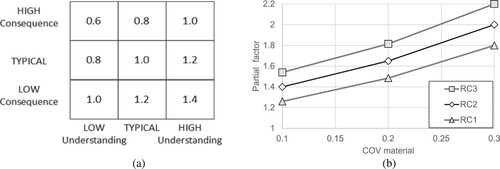
The 2021 draft version of prEN 1997–1 (CEN 2020), incorporates partly similar thinking as in Figure 9. Therein Geotechnical Categories (GC) are introduced as functions of the Consequence Class (CC) and the Geotechnical Complexity Class (GCC), as shown in Table 7. The Geotechnical Categories do not influence the partial factors but are used to specify the minimum requirement regarding: ground investigation, validation of calculation models, supervision, inspection, monitoring, designer qualification and experience and amount of reporting. However, the draft introduces consequence factors K_M that are applied to the partial factors on soil strength. As the K_M factors depend only on the consequence of failure and aim to provide different target reliability index values, the application of the K_M factors has essentially the same effect on the partial factor values as have the consequence and reliability class (RC) in Figure 9a) and b) respectively, i.e. the vertical axis in both graphs. Note, in Figure 9a) the factors are multiplier resistance factors, while in Figure 9b) the factors are divisor partial factors adopted in Eurocode 7 in general.

Table 7. Definition of Geotechnical Categories (GC) based on Consequence Classes (CC) and Geotechnical Complexity Classes (GCC) according to draft prEN-1997-1 (CEN 2020).

Consequence Class (CC)	Geotechnical Complexity Class (GCC)
	Lower (GCC1)	Normal (GCC2)	Higher (GCC3)
Higher (CC3)	GC2	GC3	GC3
Normal (CC2)	GC2	GC2	GC3
Lower (CC1)	GC1	GC2	GC2

Ching, Phoon, and Yu (2014) showed that the value of site investigation can be monetised using simplified RBD. By doing so, site investigation will be viewed as an investment rather than as a cost. Similar gains can also be achieved with approaches like those represented in Figure 9. By improving the understanding and reducing the uncertainties lower partial factors can be used to achieve the same reliability but with lower costs. In all countries, site investigation is kept as a minimum purely to satisfy building regulations rather than geotechnical needs. This state of affairs is detrimental to the advancement of the industry and to our knowledge, there is no persuasive and defensible strategy to change this attitude among cost-conscious clients. The potential for RBD to change this state of affairs is not well appreciated. This issue has even become pressing recently, because keeping site investigation to a minimum is out of alignment with digital transformation that views data as an asset.

A characteristic feature of geotechnical calculations is that they are often highly non-linear. As pointed out by Phoon (2017), a large COV in an input parameter may not propagate to a large COV in the response. For other cases, a minor change of input may have a big influence on the output. Honjo et al. (2009) opined that the choice of a characteristic value that is considerably different from its mean value may result in the predicted behaviour of the designed structure being very different from the most likely behaviour of the actual structure. Honjo et al. (2009) further emphasised the philosophy that a design engineer should keep track of the most likely behavior of the structure to the last stage of the design as much as possible. To follow this idea, the characteristic soil properties should be best estimate values rather than fractiles. On the other hand, Simpson (2011) advocated the need to imagine worst credible situations or values based on a reasonable and informed engineering assessment. The choice between “most likely” and “worst credible” scenarios is intrinsically related to deterministic analysis, where an engineer is compelled to perform only one analysis based on one set of inputs. This dichotomy does not exist in reliability analysis, where all scenarios from “most likely” to “worst credible” are considered.

In relation to the notion of a worst credible value and similar ideas, it can also be asked, do we always know on what side a cautious estimate is with respect to the occurrence of a limit state. In structural design mean stiffness values are used for the majority of cases also for ULS calculations. The reason being that it is often impossible to anticipate if an upper or a lower value would be more cautious when analysing a complicated structural model. The same argument is very much true also for many complex soil-structure interaction problems. It is not necessarily evident beforehand whether an upper or lower value is cautious, especially not which combination of upper and lower values is the governing one. The notion of a cautious or worst credible value is likely to be practical only for relatively common and familiar Geotechnical Category 2 ULS problems where low strengths are clearly cautious or worst credible estimates. The notion of a worst credible situation (in contrast to a worst credible value) is related to the occurrence of a limit state. It is conceptually similar to the ITP2 method presented by Ching et al. (2020b). Translating this concept to a familiar non-probabilistic calculation procedure that can appeal to practitioners is not straightforward.

6. Conclusions

The baseline design method, as in EN 1997–1 (CEN 2004), is empirical. Yet Eurocode 7 is not seen as a simple and transparent design code, and the resulting probability of failure may vary even beyond that implied by working stress design. The Quantile Value Method (QVM) (Ching and Phoon 2011) can be viewed as a theoretical basis for this baseline method. Phoon (2017) opined that the QVM is a “strategy of keeping the resistance factor constant while adjusting the characteristic resistance to handle different site conditions bears some similarity to the Eurocode 7 partial factor approach in EN 1997–1 (CEN 2004). However, QVM is a form of simplified RBD while Eurocode 7 is not in the sense that it does not seek to meet an explicit target reliability index approximately. The design quantile in QVM may be larger or smaller than 5% (the recommended value in Eurocode 7), depending on the target reliability index. EN 1990 (CEN 2002) recommended different reliability indices for different reliability classes (Table B2) and limit states (Table C2). The main takeaway here is that geotechnical design is less amenable to standardisation than structural design and the engineer should be able to exercise his/her discretion to adjust the partial material and resistance factors and/or related characteristic values to suit a particular site and other localised aspects of geotechnical practice. A completely prescriptive approach in which the engineer is deprived of any room to adjust the partial material and resistance factors and the related characteristic values runs counter to the notion that each site is distinct and hence a separate site investigation is warranted”.

To accommodate all this in a single safety approach is fraught with significant difficulties, both practical and theoretical. Instead, a framework allowing for different approaches with different levels of sophistication and accuracy could be applied. As an example, a three-level approach could be as follows.

(1) Variable partial factor approach

In ULS design, partial factor values are chosen depending on the level of general understanding and consequence of failure and they are scaled with the aid of RBD to achieve consistent level for probability of failure. In SLS design, best estimate input parameter values are used in analyses and the outcomes, e.g. settlements, are multiplied by factors to account for the general understanding and consequence of exceedance of the serviceability limit.

(2) Semi RBD (Phoon and Ching 2016)

This includes many new methods, like the simplified QVM-ERD for multiple correlated input parameters discussed above. The methods need to be sophisticated enough to overcome the deficiencies of Approach 1, yet transparent and simple to use.

(3) Full RBD (Wang et al. 2016)

When sufficient data are available, the application of full RBD accounting for all the true uncertainties involved should be encouraged.

The authors believe that any design standard adopted for future needs should include the following two principles; a) all parties in a project should be engaged to reduce uncertainties to an acceptable level, and b) to achieve a) all parties should be engaged to share and actively use all data available. These principles are more aligned to the spirit of digital transformation taking place in all industries.

Acknowledgements

The authors are grateful to Professor Limin Zhang, Editor-in-Chief of Georisk, for his kind invitation to submit this paper as a Spotlight Article. The authors have received many valuable comments and suggestions from the following people: Professor Trevor Orr, Dr. Johan Spross and Dr. Timo Schweckendiek. Their contribution is highly appreciated, making valuable improvements to the paper. We are especially grateful to Professor Trevor Orr and the anonymous reviewers for offering many insightful comments that have improved this paper significantly.

Disclosure statement

No potential conflict of interest was reported by the author(s).

References

- Bedi, A., and T. L. L. Orr. 2014. Rock Engineering and Rock Mechanics: Structures in and on Rock Masses (pp.1517–1523). doi:https://doi.org/10.1201/b16955-264.
- Bond, A., and A. Harris. 2008. Decoding Eurocode 7. London: Taylor and Francis.
- Cami, B., S. Javankhoshdel, K. K. Phoon, and J. Ching. 2020. “Scale of Fluctuation for Spatially Varying Soils: Estimation Methods and Values. ASCE-ASME Journal of Risk and Uncertainty in Engineering Systems.” Part A: Civil Engineering 6 (4): 03120002.
- CAN/CSAS614:2014. Canadian Highway Bridge Design Code. Mississauga, Ontario, Canada: Canadian Standards Organization.
- CEN. 2002. EN 1990: Eurocode - Basis of structural design. Comité Européen de Normalisation.
- CEN. 2004. EN 1997-1: Geotechnical design – Part 1: General rules. Comité Européen de Normalisation.
- CEN. 2020. prEN 1997-1 Geotechnical design – General rules (PT6) Oct2020. Comité Européen de Normalisation.
- Ching, J., Y. G. Hu, and K. K. Phoon. 2016. “On Characterizing Spatially Variable Shear Strength Using Spatial Average.” Probabilistic Engineering Mechanics 45: 31–43.
- Ching, J., W. H. Huang, and K. K. Phoon. 2020. “3D Probabilistic Site Characterization by Sparse Bayesian Learning. Journal of Engineering Mechanics.” ASCE 146 (12): 04020134.
- Ching, J., S. W. Lee, and K. K. Phoon. 2016. “Undrained Strength for a 3D Spatially Variable Clay Column Subjected to Compression or Shear.” Probabilistic Engineering Mechanics 45: 127–139.
- Ching, J., and K. K. Phoon. 2011. “A Quantile-Based Approach for Calibrating Reliability-Based Partial Factors.” Structural Safety 33: 275–285.
- Ching, J., and K. K. Phoon. 2013a. “Mobilized Shear Strength of Spatially Variable Soils Under Simple Stress States.” Structural Safety 41: 20–28.
- Ching, J., and K. K. Phoon. 2013b. “Probability Distribution for Mobilized Shear Strengths of Spatially Variable Soils Under Uniform Stress States.” Georisk: Assessment & Management of Risk for Engineered Systems & Geohazards 7 (3): 209–224.
- Ching, J., and K. K. Phoon. 2013c. “Multivariate Distribution for Undrained Shear Strengths Under Various Test Procedures.” Canadian Geotechnical Journal 50 (9): 907–923.
- Ching, J., and K. K. Phoon. 2015. Constructing Multivariate Distribution for Soil Parameters. Chapter 1, Risk and Reliability in Geotechnical Engineering, CRC Press, 3–76.
- Ching, J., K. K. Phoon, and Y.-C. Chen. 2010. “Reducing Shear Strength Uncertainties in Clays by Multivariate Correlations.” Can. Geotech. J 47: 16–33. doi:https://doi.org/10.1139/T09-074.
- Ching, J., K. K. Phoon, K. F. Chen, T. L. L. Orr, and H. R. Schneider. 2020b. “Statistical Determination of Multivariate Characteristic Values for Eurocode 7.” Structural Safety 82: 101893.
- Ching, J., K. K. Phoon, J. R. Chen, and J. Park. 2013. “Robustness of Constant LRFD Factors for Drilled Shafts in Multiple Strata.” Journal of Geotechnical and Geoenvironmental Engineering 139 (7): 1104–1114.
- Ching, J., K. K. Phoon, and P. H. Kao. 2014. “Mean and Variance of Mobilized Shear Strength for Spatially Variable Soils Under Uniform Stress States. Journal of Engineering Mechanics.” ASCE 140 (3): 487–501.
- Ching, J., K. K. Phoon, Z. Khan, D. M. Zhang, and H. W. Huang. 2020a. “Role of Municipal Database in Constructing Site-Specific Multivariate Probability Distribution.” Computers and Geotechnics 124: 103623.
- Ching, J., K. K. Phoon, and Y. K. Pan. 2017. “On Characterizing Spatially Variable Soil Young’s Modulus Using Spatial Average.” Structural Safety 66: 106–117.
- Ching, J., K. K. Phoon, and J. J. Yang. 2015. “Role of Redundancy in Simplified Geotechnical Reliability-Based Design - a Quantile Value Method Perspective.” Structural Safety 55: 37–48.
- Ching, J., K. K. Phoon, and J. W. Yu. 2014. “Linking Site Investigation Efforts to Final Design Savings with Simplified Reliability-Based Design Methods.” Journal of Geotechnical and Geoenvironmental Engineering. ASCE 140(3): 04013032.
- Ching, J., S. P. Sung, and K. K. Phoon. 2017. “Worst Case Scale of Fluctuation in Basal Heave Analysis Involving Spatially Variable Clays.” Structural Safety 68: 28–42.
- Ching, J., X. W. Tong, and Y. G. Hu. 2016. “Effective Young’s Modulus for a Spatially Variable Elementary Soil Mass Subjected to a Simple Stress State.” Georisk: Assessment & Management of Risk for Engineered Systems & Geohazards 10 (1): 11–26.
- Ching, J., S. Wu, and K. K. Phoon. 2021. “Constructing Quasi-Site-Specific Multivariate Probability Distribution Using Hierarchical Bayesian Model. Journal of Engineering Mechanics.” ASCE 147 (10): 04021069.
- Ching, J., Z. Y. Yang, and K. K. Phoon. 2021. “Dealing with non-Lattice Data in Three-Dimensional Probabilistic Site Characterization. Journal of Engineering Mechanics.” ASCE 147 (5): 06021003.
- Denver, H., and N. K. Ovesen. 1994. Assesment of Characteristic Values for Soil Parameters for Design. New Delhi, India: XIII ICSMFE 1994.
- Di Buò, B., J. Selänpää, T. Länsivaara, and M. D’Ignazio. 2018. Evaluation of Existing CPTu based Correlations for Deformation Properties of Soft Clays. CPT18 - 4th International Symposium on Cone Penetration Testing, Delft.
- Fenton, G. A., and D. V. Griffiths. 2008. Risk Assessment in Geotechnical Engineering. Hoboken, N.J.: John Wiley & Sons.
- Fenton, G. A., F. Naghibi, D. Dundas, R. J. Bathurst, and D. V. Griffiths. 2016. “Reliability-based Geotechnical Design in 2014 Canadian Highway Bridge Design Code.” Can. Geotech. J 53: 236–251. doi:https://doi.org/10.1139/cgj-2015-0158.
- Hansen, J. B. 1965. “Philosophy of Foundation Design: DesignCriteria, Safety Factors and Settlement Limits.” Paper presented at the proceedings, symposium on bearing capacity and settlement of foundations, Duke University, Durham, 1–13.
- Hicks, M. A. 2013. “An Explanation of Characteristic Values of Soil Properties in Eurocode 7.” In Modern Geotechnical Design Codes of Practice, edited by P. Arnold, G. A. Fenton, M. A. Hicks, T. Schweckendiek, and B. Simpson, 36–45. Amsterdam: IOS Press.
- Hicks, M. A., and J. D. Nuttall. 2012. Influence of Soil Heterogeneity on Geotechnical Performance and Uncertainty: A Stochastic View on ec7. In Proceedings of 10th International ProbabilisticWorkshop, Stuttgart, Germany, pp. 215–227.
- Hicks, M. A., and K. Samy. 2002. “Reliability-based Characteristic Values: a Stochastic Approach to Eurocode 7.” Ground Engineering 35 (12): 30–34.
- Hicks, M. A., D. Varkey, A. P. van den Eijnden, T. de Gast, and P. J. Vardon. 2019. “On Characteristic Values and the Reliability-Based Assessment of Dykes.” Georisk: Assessment & Management of Risk for Engineered Systems & Geohazards 13 (4): 313–319.
- Honjo, Y., K. L. T. Chung, T. Hara, M. Shirato, M. Suzuki, and Y. Kikuchi. 2009. “Code Calibration in Reliability Based Design Level I Verification Format for Geotechnical Structures.” Geotechnical Risk and Safety – Honjo et al. (eds). 2009 Taylor & Francis Group, London, ISBN 978-0-415-49874-6. Pages 435–452.
- Hu, Y. G., and J. Ching. 2015. “Impact of Spatial Variability in Soil Shear Strength on Active Lateral Forces.” Structural Safety 52: 121–131.
- Institution of Civil Engineers. 2017. State of the Nation 2017: Digital Transformation. London. https://www.ice.org.uk/getattachment/news-and-insight/policy/state-of-the-nation-2017-digital-transformation/ICE-SoN-Report-Web-Updated.pdf.aspx.
- Janbu, N. 1995. Deformation of Soils with Collapsible Grain Structure. The Ian Boyd Donald Symposium on Modern developments in geomechanics, Monash University, Australia, pp. 127–137. Published also in Bulletin 29, Department of Geotechnical Engineering, Norwegian University of Science and Technology.
- Johnson, N. L. 1949. “Systems of Frequency Curves Generated by Methods of Translation.” Biometrika 36: 149–176.
- Knuuti, M., and T. Länsivaara. 2019. Performance of Variable Partial Factor approach in a slope design. In 13th International Conference on Applications of Statistics and Probability in Civil Engineering(ICASP13), Seoul, South Korea, May 26–30, 2019. doi:https://doi.org/10.22725/ICASP13.475.
- Länsivaara, T. 2000. Painumalaskentamenetelmien käyttökelpoisuuden arviointi. Tielaitoksen selvityksiä, no. 44, Tiehallinto, Helsinki (in Finnish).
- Länsivaara, T. 2012. Some Aspects on Creep and Primary Deformation Properties of Soft Sensitive Scandinavian Clays. in Proceedings of the 16th Nordic Geotechnical Meeting NGM 2012, 9–12 May 2012, Copenhagen, Denmark. 16th Nordic Geotechnical Meeting, vol. 1–2, Danish Geotechnical Society, Copenhagen, Denmark, pp. 397–404.
- Länsivaara, T., and M. Knuuti. 2015. A Proposal for some Modifications of EN 1997-1 Design Approaches. in Fifth International Symposium on Geotechnical Safety and Risk (ISGSR): Rotterdam, The Netherlands 13–16 October 2015. IOS Press, pp. 486–491, International Symposium on Geotechnical Safety and Risk, Netherlands, 1/11/10.
- Länsivaara, T., and T. Poutanen. 2014. “Safety Concepts for Slope Stability.” In Landslides in Sensitive Clays: From Geosciences to Risk Management. Advances in Natural and Technological Hazards Research, vol. 36, edited by J.-S. L'Heureux, A. Locat, S. Leroueil, D. Demers, and J. Locat, 395–407. Netherlands: Springer. doi:https://doi.org/10.1007/978-94-007-7079-9_31.
- Li, D. Q., S. B. Wu, C. B. Zhou, and K. K. Phoon. 2012. “Performance of Translation Approach for Modeling Correlated non-Normal Variables.” Structural Safety 39: 52–61.
- Low, B. K. 2015. “Reliability-based Design: Practical Procedures, Geotechnical Examples, and Insights.” Chapter 9 in Risk and Reliability in Geotechnical Engineering. Edited by Phoon, K. K. & Ching, J. CRC Press.
- Lunne, T., T. Berre, and S. Strandvik. 1997. “Sample Disturbance Effects in Soft Low Plastic Norwegian Clay.” In Proceeding of the International Symposium on Recent Developments in Soil and Pavement Mechanics. Rio De Janeiro, Brazil, 81–102.
- Müller, R. 2013. “Probabilistic Stability Analysis of Embankments Founded on Clay.” Doctoral Thesis. Division of Soil and Rock Mechanics, Department of Civil and Architectural Engineering, Royal Institute of Technology, Stockholm.
- Müller, R., S. Larsson, and J. Spross. 2014. “Extended Multivariate Approach for Uncertainty Reduction in the Assessment of Undrained Shear Strength in Clays.” Canadian Geotechnical Journal 51: 231–245. doi:https://doi.org/10.1139/cgj-2012-0176.
- Müller, R., S. Larsson, and J. Spross. 2016. “Multivariate Stability Assessment During Staged Construction.” Canadian Geotechnical Journal 53: 603–618. doi:https://doi.org/10.1139/cgj-2015-0037.
- National Research Council. 1995. Probabilistic Methods in Geotechnical Engineering. Washington, DC: National Academies Press.
- Orr, T. L. L. 2015. Managing Risk and Achieving Reliable Geotechnical Designs using Eurocode 7. Chapter 10 in Risk and Reliability in Geotechnical Engineering. Edited by Phoon, K. K. & Ching, J. CRC Press.
- Phoon, K. K. 2017. “Role of Reliability Calculations in Geotechnical Design.” Georisk: Assessment and Management of Risk for Engineered Systems and Geohazards 11 (1): 4–21.
- Phoon, K. K. 2018. “Editorial for Special Collection on Probabilistic Site Characterization. ASCE-ASME Journal of Risk and Uncertainty in Engineering Systems.” Part A: Civil Engineering 4 (4): 02018002.
- Phoon, K. K. 2020. “The Story of Statistics in Geotechnical Engineering.” Georisk: Assessment & Management of Risk for Engineered Systems & Geohazards 14 (1): 3–25.
- Phoon, K. K., and J. Ching. 2013. Is Site Investigation an Investment or Expense? - A Reliability Perspective. Proceedings, 18th Southeast Asian Geotechnical Conference (18SEAGC) & Inaugural AGSSEA Conference (1AGSSEA), 29–31 May 2013, Singapore, 25–43.
- Phoon, K. K., and J. Ching. 2016. Semi-probabilistic Reliability-based design. Chapter 6, Reliability of Geotechnical Structures in ISO2394, Eds. K. K. Phoon & J. V. Retief, CRC Press/Balkema, 159–192.
- Phoon, K. K., and J. Ching. 2021. “Project DeepGeo - Data-Driven 3D Subsurface Mapping.” Journal of GeoEngineering 16 (2): 47–59.
- Phoon, K. K., J. Ching, and J. R. Chen. 2013. “Performance of Reliability-Based Design Code Formats for Foundations in Layered Soils.” Computers and Structures 126: 100–106.
- Phoon, K. K., J. Ching, and T. Shuku. 2021. Challenges in Data-driven Site Characterization. Georisk, doi:https://doi.org/10.1080/17499518.2021.1896005.
- Phoon, K. K., and F. H. Kulhawy. 2008. Serviceability Limit State Reliability-based Design. Chapter 9, Reliability-Based Design in Geotechnical Engineering: Computations and Applications, Taylor & Francis, UK, 344–383.
- Phoon, K. K., F. H. Kulhawy, and M. D. Grigoriu. 1995. Reliability-based Design of Foundations For Transmission Line Structures. Report TR-105000, Electric Power Research Institute, Palo Alto.
- Phoon, K. K., F. H. Kulhawy, and M. D. Grigoriu. 2003a. “Multiple Resistance Factor Design (MRFD) for Spread Foundations. Journal of Geotechnical and Geoenvironmental Engineering.” ASCE 129 (9): 807–818.
- Phoon, K. K., F. H. Kulhawy, and M. D. Grigoriu. 2003b. “Development of a Reliability-Based Design Framework for Transmission Line Structure Foundations. Journal of Geotechnical and Geoenvironmental Engineering.” ASCE 129 (9): 798–806.
- Phoon, K. K., J. V. Retief, J. Ching, M. Dithinde, T. Schweckendiek, Y. Wang, and L. M. Zhang. 2016. “Some Observations on ISO2394:2015 Annex D (Reliability of Geotechnical Structures).” Structural Safety 62: 24–33.
- Phoon, K. K., and C. Tang. 2019. “Characterization of Geotechnical Model Uncertainty.” Georisk: Assessment & Management of Risk for Engineered Systems & Geohazards 13 (2): 101–130.
- Prästings, A., J. Spross, and S. Larsson. 2019. “Characteristic Values of Geotechnical Parameters in Eurocode 7.” Proceedings of the Institution of Civil Engineers – Geotechnical Engineering 172 (4): 301–311. doi:https://doi.org/10.1680/jgeen.18.00057.
- Ravindra, M. K., and T. V. Galambos. 1978. ““Load and Resistance Factor Design for Steel”, Journal of Structural Division.” ASCE 104 (ST9): 1337–1353.
- Schneider, H. R., and M. A. Schneider. 2013. Dealing with Uncertainties in EC7 with Emphasis on Determination of Characteristic Soil Properties, Modern Geotechnical Design Codes of Practice, eds. P. Arnold, G.A. Fenton, M.A. Hicks, T. Schweckendiek and B. Simpson, IOS Press, Amsterdam, pp87–101.
- Simpson, B. 2011. “Reliability in Geotechnical Design – some Fundamentals.” Proceedings, Third International Symposium on Geotechnical Safety & Risk, Federal Waterways Engineering and Research Institute, Germany, 393–399.
- Simpson, B., and R. Driscoll. 1998. Eurocode 7: A Commentary. Construction research communications Ltd.
- Student. 1908. The Probable Error of a mean. Biometrika, Vol 6, pp1–25.
- Tabarroki, M., J. Ching, K. K. Phoon, and Y. Z. Chen. 2021. Mobilisation-based Characteristic Value of Shear Strength for Ultimate Limit States, Georisk: Assessment & Management of Risk for Engineered Systems & Geohazards, in press.
- Tang, C., and K. K. Phoon. 2021. Model Uncertainties in Foundation Design. Boca Raton: CRC Press.
- Vanmarcke, E. H. 1977. “Probabilistic Modeling of Soil Profiles.” ASCE Journal of the Geotechnical Engineering Division 103 (11): 1227–1246.
- Vanmarcke, E. 1983. Random Fields: Analysis and Synthesis. Cambridge, USA: The MIT Press.
- Vanmarcke, E. 2010. Random Fields, Analysis and Synthesis. Singapore: World Scientific Publishing Co. Pte. Ltd.
- Wang, Y., T. Schweckendiek, W. P. Gong, T. Y. Zhao, and K. K. Phoon. 2016. “Direct Probability-based Design Methods.” Chapter 7, Reliability of Geotechnical Structures in ISO2394, Eds. K. K. Phoon & J. V. Retief, CRC Press/Balkema, 2016, 193–226.
- Wang, Y., T. Zhao, and Z. Cao. 2015. “Determination of Soil Property Characteristic Values from Standard Penetration Tests.” 12th International Conference on Applications of Statistics and Probability in Civil Engineering, ICASP12 Vancouver, Canada, July 12–15, 2015.
- Zhang, L., H. T. Tang, L. Zhang, and J. Zheng. 2004. “Reducing Uncertainty of Prediction from Empirical Correlations.” Journal of Geotechnical and Geoenvironmental Engineering 130 (5): 526–534. doi:https://doi.org/10.1061/(ASCE)1090-0241(2004)130:5(526).