Reliability assessment of open-source multiscale landslide susceptibility maps and effects of their fusion

ABSTRACT

Several landslide susceptibility (LS) maps at various scales of analysis have been performed with specific zoning purposes and techniques. Supervised machine learning algorithms (ML) have become one of the most diffused techniques for landslide prediction, whose reliability is firmly based on the quality of input data. Site-specific landslide inventories are often more accurate and complete than national or worldwide databases. For these reasons, detailed landslide inventory and predisposing variables must be collected to derive reliable LS products. However, high-quality data are often rare, and risk managers must consider lower-resolution available products with no more than informative purposes. In this work, we compared different ML models to select the most accurate for large-scale LS assessment within the Municipality of Rome. The ExtraTreesClassifier outperformed the others reaching an average F1-score of 0.896. Thereafter, we addressed the reliability of open-source LS maps at different scales of analysis (global to regional) by means of statistical and spatial analysis. The obtained results shed light on the difference in hazard zoning depending on the scale and mapping unit. An approach for low-resolution LS data fusion was attempted, assessing the importance of the adopted criteria, which increased the ability to detect occurred landslides while maintaining precision.

KEYWORDS:

• Landslide susceptibility
• machine learning
• map scale
• data fusion
• Rome

1. Introduction

Shallow landslides are slope instabilities which involve the most superficial deposits, mainly colluvium, rather than bedrock formations (Baeza and Corominas 2001; Bordoni et al. 2021). They are most frequently triggered by extreme rainfall and can be densely distributed across small catchments (Hungr, Leroueil, and Picarelli 2014). In urban areas, even in case of small-sized, shallow slope failures, their occurrence as spatially distributed clusters as frequent as their triggering rainfall event is capable of tearing the physical structure as well as the network of socio-economic, cultural, material and immaterial relations that make up the life of cities (Iadanza et al. 2009; 2013; Salvati et al. 2010; Trigila, Iadanza, Munafò, et al. 2015; Trigila, Iadanza, and Spizzichino 2010). This is due to their rapid or extremely rapid movement and intrinsic damage potential both in terms of human and economic losses (Trigila, Iadanza, Esposito, et al. 2015). The recent expansion of urban areas entails a significant soil cover consumption and demands correct and sustainable urban planning to face off with the delineation of landslide-prone areas. Human pressure has modified geological, geomorphological, and hydrological features of original terrains through centuries, acting on topography, stratigraphy, and even geotechnical properties of the subsurface, by developing networks of superficial and underground structures, modifying or obliterating water streams (Luberti et al. 2018). Therefore, the importance of the analysis and evaluation of hazard sources for risk mitigation actions in urban areas is evident. Since the 1980s, the role of urban planning in the knowledge and prevention of landslides has expanded considerably. Nowadays, landslide hazard analysis is usually mandatory to approach proper land use planning and management (Mateos et al. 2020). Nevertheless, in some cases regulatory plans lack detailed thematic mapping of geohazard-related data (Cui et al. 2019) despite cities are frequently affected by landslides and exposed to high risk (Crosta et al. 2005; Kiersch 1964; Martino et al. 2019; Mazzanti and Bozzano 2011; Tonini et al. 2022).

Landslide hazard management can be developed at different spatial scales and with different methods with increasing degrees of sophistication and different zoning purposes (Fell et al. 2008), which can be informative or advisory up to statutory and regulatory or devoted to engineering design (Cascini 2008; Corominas et al. 2013; Flentje et al. 2007), whose reliability is strongly based on quality and completeness of the available landslide catalogues.

Several open-source landslide inventories exist worldwide; however, the amount and quality of available data may be inadequate to build accurate large-scale predictive models. Open-source landslide inventories may have incomplete spatial and temporal information and heterogeneous features, which affirms the need to integrate them to gain reliability (Mastrantoni et al. 2022). Alternatively, recent developments have shown the potential of SAR satellite imagery for multitemporal mapping of landslides (Bhuyan et al. 2023).

To achieve a proper prediction of landslide susceptibility (LS), landslide inventory data must be processed together with predisposing and preparatory factors to model hidden patterns, thus suggesting new potentially unstable slopes (Basu and Pal 2018; Corominas et al. 2013; van Westen, Castellanos, and Kuriakose 2008; Vijith et al. 2014). In the past decades, various approaches to determine the degree of LS have been proposed and applied by employing heuristic, data-driven and physically based methods for various types of landslides at different observation scales (Brabb 1984; Fell et al. 2008; Guzzetti et al. 1999; Günther et al. 2014; Kainthura and Sharma 2022; Luo et al. 2022; Ngadisih, Bhandary, and Dahal 2014; Soeters and Van Westen 1996). Among data-driven approaches, multivariate analysis is one of the most sophisticated techniques for LS assessment. The spatial distribution of landslides is predicted through the estimation of the relationship between several independent predisposing factors and response variables, relying on the information on previous landslide and non-landslide samples (Persichillo et al. 2017; Su et al. 2022). A recent and important statistical improvement for LS studies is the advance in machine learning algorithms (ML). During the past two decades several models have been developed (e.g. random forest, support vector machines, artificial neural networks etc.). Although some methods performed better than others, no single method proved to be superior under all conditions (Reichenbach et al. 2018). Hence, it is not recommended to select the model in advance, but as many models as possible should be built and compared. Once obtained, the best-performing one is selected and used for landslide zoning purposes.

Since several LS maps at medium to small scale are available, understanding their potentiality and that of their integration for the prediction of stable and unstable areas may become relevant when detailed products are not yet available. Therefore, two main topics were investigated in the following: (i) the achievement of a reliable urban-scale assessment of landslide susceptibility in the Municipality of Rome and, (ii) the comparison with each available map and with the products derived by their fusion.

The exploiting of geospatial information through Machine Learning algorithms allowed us to estimate an urban-scale landslide susceptibility zoning (LSZ) for the Municipality of Rome, weighting and validating the different models adopted, selecting the most accurate one for the area of interest. The obtained result is then compared with open-source, regional, national, European, and global scale susceptibility maps to quantitatively assess their similarity and accuracy, and therefore the overall reliability. The fusion of LSZ products based on different analysis unit and resolution was addressed to evaluate the information gain or loss of the obtained output. By merging the LSZ maps we wanted to assess whether the adopted data fusion criteria can lead to a significant increase in accuracy and reliability of small-scale maps (i.e. global to national) generally available worldwide, thus potentially rising their applicability from informative to at least advisory.

2. Case study

The study area corresponds to the Municipality of Rome, extending to about 1287 km². The area within the city of Rome has experienced a series of geological processes over the last hundreds of thousands of years that encompass volcanic activity and relative sea-level changes that have influenced the erosional and depositional stages of the lower part of the Tiber River catchment. Sedimentary complexes deposited during the Plio-Pleistocene are constituted by both marine and continental deposits (e.g. clays, sands and conglomerates of alluvial deposits) outcropping the hills on the right bank of the Tiber River. They are superimposed by an alternating succession of volcanic products and continental sediments. Volcanic products erupted about 600k years ago by monogenic and polygenic complexes of the Alban Hills and the Sabatini volcanic district. Recent alluvial deposits of the Tiber River and its tributaries have filled the valley reaching thicknesses of tens of metres (Bozzano et al. 2000; Funiciello and Giordano 2008; Parotto 2008). The left and right embankments of the Tiber River valley have distinct geological units, thus resulting in different responses to natural and anthropogenic hazard processes, including subsidence (Bozzano et al. 2015), sinkholes (Ciotoli et al. 2014; Esposito et al. 2021), urban and fluvial floods and landslides (Amanti, Chiessi, and Guarino 2012; Del Monte et al. 2016), that affected the area over the years.

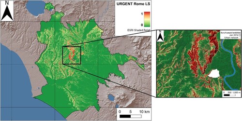
Landslides in Rome are mainly represented by shallow landslides (soil slips and translational slides) with reduced and comparable volumes. Recently occurred landslides in Rome are characterised by an average area of 2.1 × 10³ m², that due to the shallow position of the sliding surfaces (2–5 m) correspond to an average volume of 5 × 10³ m³ as order of magnitude (Alessi et al. 2014; Del Monte et al. 2016). Additionally, ephemeral hydraulic circulation built up along permeability contrasts between volcanic, or debris covers overlying sedimentary deposits, may induce transient seeping that reduces slope stability. The Monte Mario and Monte Ciocci hills are the areas where most of the recorded landslides have occurred (Figure 1). Their proneness to landsliding might be related to high slope angles formed of the Monte Vaticano and Monte Mario Formations, which consist of a thick succession of clays, silty-clays, and silty-sands highly sensitive to shallow and translational landslides. The weathering of these deposits produced unsaturated shallow soil covers, which have been proven to host ground instabilities (Schilirò et al. 2019).

Figure 1. Number of landslide events per geomorphological slope unit (Alvioli, Guzzetti, and Marchesini 2020) within the Municipality of Rome (a); percentage of landslides by type of failure, as defined by Hungr, Leroueil, and Picarelli (2014) (b); slope angle distribution of landslide events by type (c). Slope units are shown for non-flat areas only.

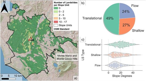
According to Esposito et al. (2023), the city of Rome has experienced at least 566 landslide events over the last century, 356 of which are reported as translational, flow or shallow landslides (Figure 1b,c). These landslides have almost always been associated with heavy rainfall, among which sixty-seven occurred during the exceptional rainfall event registered from 31 January to 2 February 2014 (Alessi et al. 2014). This event and the landslide related damages declare Rome’s susceptibility to geological hazards, which can interact with socio-economic activities, posing relevant risk conditions, and causing a significant impact, as documented by the service and road infrastructure interruption after the event, whose consequences lasted for months. Although landslide hazard in Rome, as well as in other major cities in Italy, is widely known, it still lacks urban-scale regulatory or advisory landslide susceptibility zonation, except for national scale susceptibility or hazard indicators (Iadanza et al. 2021; Trigila et al. 2013).

3. Materials & methods

3.1. Urban-scale assessment of landslide susceptibility

Analysis based on ML methods needs reliable data on which the model is based. The main prerequisite is information on the spatial occurrence of landslide events (van Westen, Castellanos, and Kuriakose 2008) together with conditioning factors picked because of their expected relationship with the occurrence of slope failures. Although landslide inventories are often incomplete in spatial and temporal terms, integration, cross-validation, and processing of open-source databases produced at different scales of observation are required to reduce bias before training the predictive models to be compared. In this study, the standardised and boosted landslide database of Rome was used to train different supervised ML algorithms.

The database contains both Landslide Initiation Points (LIP) and related polygons representing the area involved. The best performing model was then employed to estimate the LS level for the whole area, thus resulting in the urban-scale LSZ which in this study is referred to as “URGENT Rome”. It is developed within the PRIN project entitle “URGENT – URban Geology and geohazards: Engineering geology for safer, resilieNt and smart ciTies”.

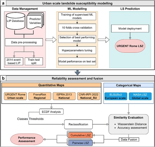
Figure 2(a) describes the pipeline implemented in this study to achieve the urban-scale shallow landslide susceptibility map of Rome.

Figure 2. Workflow developed to obtain an urban-scale landslide susceptibility zoning of Rome territory (a), and reliability assessment of open-source LS maps at different scales of observation (b).

3.1.1. Data pre-processing

All ML algorithms use some input data to create outputs. Input data comprise features, which are usually in the form of structured columns. Algorithms require features with some specific characteristics to work properly. Here, the need to feature engineering arises. Feature engineering was performed with two main goals: (1) preparing the proper input dataset, compatible with the ML algorithm requirements (i.e. tidy structure), and (2) improving the performance of the models.

Data about terrain, lithological, hydrological, soil, roads and streams were selected as potential predictor variables (Table 1). A total of 20 variables are included, of which 14 represent terrain features derived from the 5 m resolution DTM. Distances from roads, hydraulic permeability limits (i.e. hydrogeological units that cause significant contrast in hydraulic conductivity) and water streams were also computed. The remaining are categorical variables representing litho-technical units and urban land characteristics.

Table 1. List of variables deemed predictors of landslide susceptibility in Rome.

Variable	Abbreviation	Description
Digital Terrain Model	DTM	5 × 5 m DTM model derived by points and contour lines of elevation with Anudem algorithm (Hutchinson, Xu, and Stein 2011).
Slope Angle	slope	5 × 5 m slope angle map
Relative Relief	rrelief100	Difference between max and min altitude within a cell of 100 m (Oguchi 1997)
Topographic Position Index	tpi	TPI with a neighbourhood equal to 300 m
Dissection Ratio	dess_ratio	Topographic dissection within 100 m grid.
Drop	drop	Relative height within a radius of 50 m.
Aspect	aspect	Topographic aspect as degrees from north.
Aspect classes	aspect_8	Topographic aspect reclassified in 8 dials.
Curvatures	curv_plan, curv_prof, curv_tot	Planar, parallel and total curvature based on 5 × 5 m DTM
Flow Accumulation	flow_acc	Amount of upstream area draining into a cell.
Topographic Wetness Index	twi	Steady state wetness index map.
Ordinary annual rain	ord_rain	Based on rainfall analysis of 33 distributed rain gauges records (from 1951 to 2021)
Soil thickness	soil_thickness	Soil thickness based on Saulnier’s equation (Saulnier, Beven, and Obled 1997)
Land use	land_use	Regione Lazio land cover map https://dati.lazio.it/catalog/it/dataset/carta-uso-suolo-2016
Litho-technical units	litho	Based on 1:25000 lithological map of the Regione Lazio https://dati.lazio.it/catalog/it/dataset/carta-geologica-informatizzata-regione-lazio-25000
Distance to streams	dist_idro	Euclidean distance to nearest stream
Distance to roads	dist_road	Euclidean distance to nearest road.
Distance to permeability limit	dist_lim_k	Based on hydrogeological complex defined in the Hydrogeological map of Rome (La Vigna et al. 2015).

We derived litho-technical units from the official lithological map of Rome by grouping geological formations with similar geotechnical characteristics. We did not include the individual formations as a predictor variable due to the large number of categories, which would result in a high-cardinality feature. According to Maxwell et al. (2020), this allows embedding expert knowledge into the prediction. We also included land cover and soil consumption information to account for urban assets and activities. Thereafter we encoded categorical variables by replacing the original value of the feature with the frequency distribution, thus converting the feature into a numeric. Since we are dealing with rainfall-triggered shallow landslides, we took advantage of 33 distributed rain gauge records (from 1951 to 2021) to derive Thiessen polygons and their amount of ordinary annual rainfall.

All raster-based variables were then extracted at the mapped LIP and stable point locations using the Point sampling tool plugin (Jurgiel 2013) of QGIS 3 to generate tables from which to extract train, validation and test data.

Input data consist of LIPs and stable points with a ratio of 35–65%, for an overall amount of 2992 records stored as geo-dataframe. The few dated landslide records (i.e. those triggered by the heavy rainfall of 31 January 2014) were formerly split from the database and treated as event-based test samples to assess the capability of the six LSZs to correctly detect landslide occurrences.

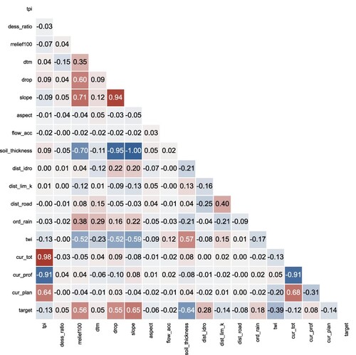
The importance of features in ML algorithms plays a very crucial role in prediction analysis in any field. First, we explored the data to select a subset of input features that would be relevant to the prediction, thus avoiding the issue of dimensionality, as some algorithms perform badly when in high dimensionality. Correlations between features, or multicollinearities, were calculated and variables were systematically removed if a pairwise correlation exceed 75%, as recommended by Kuhn and Johnson (2013). The algorithm used to filter out multicollinearity calculated a correlation matrix and the highest pairwise correlation was found (Figure 3). The variable within this pair with the lower correlation with the target variable was removed from the dataset. This was repeated until no pairwise correlation exceeded 75%. Sixteen out of 20 variables remained to be used in model training after verifying that there was no missing or redundant information.

Figure 3. Pairwise correlation of all continuous numerical features originally included in the study.

3.1.2. Machine learning modelling

Candidate models include Naïve Bayes, logistic regression, k-nearest neighbours and decision trees-based methods. The complete list of trained models can be found in Table 2. The data were split into two subsets. The former being the training set containing 80% of the data, whereas the latter being the hold-out set containing the remaining 20%. Stratified random sampling was used to account for the imbalanced binary outcome (Kotsiantis, Kanellopoulos, and Pintelas 2006). K-fold cross validation was performed on the training set to train and validate the model with ten subsets validation data.

Table 2. Machine learning classifiers being compared in this study. Abbreviations defined in this table will be used throughout the paper.

ML model	Abbreviation	Type of algorithm
Extra Trees Classifier	ET	Ensemble of decision trees
Light Gradient Boosted Machine	LightGBM	Ensemble of decision trees
Random Forest	RF	Ensemble of decision trees
Gradient Boosting Classifier	GBC	Ensemble of decision trees
Ada Boost Classifier	ADA	Ensemble of decision trees
Decision Tree	DT	Single tree structure
Logistic Regression	LR	Sigmoid function
Naïve Bayes	NB	Bayes theorem
Linear Discriminant Analysis	LDA	Linear decision boundary
K Nearest Neighbours	KNN	k-nearest neighbours vote

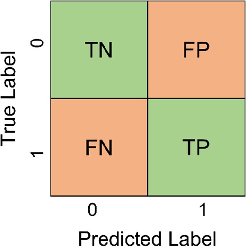
Cross-validation results were then used to compute ten confusion matrices for each model. Given a confusion matrix (Figure 4), the distribution of the overall accuracy (Equation 1), recall (Equation 2), precision (Equation 3), F1-Score (Equation 4) and ROC-AUC (Fawcett 2006) was derived. Score metrics were then used to select the best performing model to be further optimised with hyperparameters tuning. Since F1-score considers not only the number of prediction errors that the model makes, but also looks at the type of errors that are made, it works well on imbalanced data. For this reason, we chose the F1-score to select the most suitable model to predict susceptibility levels in the whole area. GridSearchCV function of the Scikit-learn library (Pedregosa et al. 2011) was exploited to determine the optimal set of hyperparameter values, thus minimising both variance and bias. To better understand and explain how the model works, we implemented the permutation feature importance method to assess feature relevance avoiding bias from categorical variables (Altmann et al. 2010).

Figure 4. Confusion matrix for binary classification where TP and TN denote the number of positive and negative examples that are classified correctly, while FN and FP denote the number of misclassified positive and negative examples respectively.

Once tested, the trained model was applied to predict the probability of each raster cell being a landslide initiation point, thus resulting in the LS map with values ranging from 0 to 1, representing minimum and maximum susceptibility respectively.

All the machine learning model development and deployment were coded in Python 3 taking advantage of Scikit-learn and PyCaret libraries among others (Ali 2020; Pedregosa et al. 2011). (1) $Accuracy={\displaystyle \frac{TP+TN}{TP+FP+FN+TN},}$(1) (2) $Recall={\displaystyle \frac{TP}{TP+FN},}$(2) (3) $Precision={\displaystyle \frac{TP}{TP+FP},}$(3) (4) $F1-score=2\times {\displaystyle \frac{Recall\times Precision}{Recall+Precision},}$(4)

3.2. Accuracy assessment and data fusion

This section focuses on evaluating and merging the available open-source LS maps originally produced at different scales of analysis to boost their performance. To this aim, the assessment of both similarity and accuracy of open-source LSZ with reference to the urban-scale map produced in this study was required. According to Cascini (2008), different scales of analysis denote different purposes. However, regional- to urban-scale susceptibility maps are often lacking. Therefore, there is a need to assess the reliability and potentials of small- to medium-scale LSZ in case more detailed studies have not yet been conducted. For that purpose, five LS maps at different scales and mapping units, including regional, national, European and global scale products, were collected and compared with the one produced in this study. Figure 2(b) illustrates maps and workflow implemented to carry out the performance assessment and to achieve multiscale-based LSZ products.

FranaRisk LSZ (Argentieri et al. 2018) covers the entire province of Rome with a cell size of 20 m. ISPRA 2013 (Trigila et al. 2013) and CNR-IRPI 2022 shallow LSZ (Loche et al. 2022) both cover the whole Italian territory but adopting different mapping units. The first is grid-based (500 m resolution) while the latter relies on geomorphological slope units (hereafter named SU). ELSUSv2 represents the official European LSZ (Wilde et al. 2018); it has a pixel size of 200 m. Lastly, NASA LSZ covers the entire globe with a grid size of 1 km (Stanley and Kirschbaum 2017).

Out of the six LS maps, two are already categorised in five classes (i.e. NASA, ELSUSv2), while the others have continuous numerical susceptibility values. Regarding the ISPRA 2013 LS map, we rescaled it in the range of 0–1 to make it comparable. The vector-based map utilising SU was rasterised to the resolution of URGENT Rome LSZ (5 m grid cell). Among the methods reported by the literature to select class thresholds (Baeza, Lantada, and Amorim 2016), we decided to focus on the capacity of the model to detect true landslides (i.e. true positives). Empirical cumulative distribution functions (ECDF) were computed specifically from the predictions made on the event-based test samples as well as on the overall landslides polygons stored in the database. Class thresholds were defined by detection rates of 10%, 15%, 25% and 50% to classify the probabilities as “very low”, “low”, “moderate”, “high” and “very high” landslide susceptibility. The detection rate percentiles were chosen following the same values adopted for ELSUSv2 Pan-European LSZ (Wilde et al. 2018). This step was necessary to standardise the LSZs and make them quantitatively comparable.

Following the LSZ reclassification, a similarity evaluation process was implemented by means of Wasserstein distance metric together with spatialised accuracy assessment. We exploited recorded landslides polygons to evaluate the ability of each LSZ to predict landslide hazardous areas by quantifying the difference between the ECDF. Furthermore, we also compared the distributions of the event-based test samples, i.e. the January 2014 rainfall-triggered landslides, related to non-ordinary conditions (Alessi et al. 2014). This was achieved by means of the Wasserstein distance metric (Piccoli and Rossi 2016). The Wasserstein Distance represents the area between the curves of the cumulative distribution of the two groups. It tells how much, on average, you should move each point of one group to get the other group, while maintaining the quantile of the points; for categorical features, it expresses the difference in classes between the tested LSZ map and a benchmark, here assumed in the URGENT Rome, which is the most detailed and updated one.

Even though these statistical approaches allow us to determine quantitatively which is the closest LS map, spatial data also needs spatial analysis to reveal trends and patterns, thus visualising the spatial location of differences and similarities. To do so, we achieved a spatialised accuracy assessment for each collected LSZ with the benchmark map (i.e. URGENT Rome). For this purpose, the respective excerpts of the categorised LSZ were binarized by merging the two highest susceptibility classes (“high” and “very high”) as susceptible areas with the rest as non-susceptible terrain in each case (Günther et al. 2014). Overlying binarized maps allow incorrectly classified terrains to be derived in terms of false positives and false negatives. This results in a new raster map for each comparison showing true/false positives and true/false negatives in the space, i.e. an accurate or inaccurate prediction. We also report the overall confusion matrix together with metrics scores, thus allowing a performance analysis of each open-source LSZ compared to URGENT Rome. The analysis ended up with an F1-score value for each LSZ which has been considered an indicator of its reliability in Rome. F1-scores were then used as weighting parameters when fusing the LS maps. Two approaches were tested (Figure 2b) with the aim to evaluate the improvement of predictive performance by data fusion approaches: firstly, a cumulative fusion of all LSZ was implemented from smallest to largest scale, assessing the performance at each step; then, a pairwise fusion was performed between the two maps built at closer scale. Equation 5 represents the adopted criteria to merge the maps, rounding decimals to the ceil value. Where LSI is the fused landslide susceptibility index; F1 and LS denote the F1-score and landslide susceptibility class relative to the i-th LSZ, respectively. (5) $LSI={\displaystyle \frac{1}{{\sum }_{i}F{1}_i}\times \sum _i(F{1}_i\times L{S}_i),}$(5)

4. Results

4.1. Urban-scale LSZ

F1 scores calculated from the validation folds of cross-validation phase for each separate model are provided in Figure 5. Table 3 represents performance scores based on the 10 independent validation sets of candidate models. The best four models (i.e. ET, LightGBM, RF and GBC) are characterised by a distribution of F1 scores always greater than 0.8, with the ET model standing out better in the mean and maximum value, and throughout the overall distribution (i.e. lower variance). The other models have lower scores both in terms of mean values and whisker length, with KNN being the worst. By considering also other metrics the ET model remains the best among candidates.

Figure 5. Distribution of cross-validation F1 scores obtained during model training.

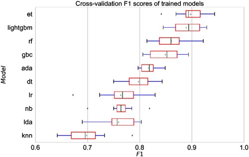
Table 3. The mean and standard deviation (SD) of scoring metrics resulting from K-fold cross validation analysis for candidate models. Data are sorted by F1 score.

Model	Accuracy		AUC		Recall		Precision		F1
	Mean	SD	Mean	SD	Mean	SD	Mean	SD	Mean	SD
et	0.933	0.018	0.979	0.007	0.906	0.034	0.886	0.034	0.896	0.028
lightgbm	0.928	0.019	0.977	0.006	0.903	0.033	0.876	0.043	0.889	0.029
rf	0.915	0.019	0.970	0.009	0.875	0.032	0.861	0.034	0.868	0.029
gbc	0.904	0.017	0.964	0.007	0.856	0.046	0.843	0.027	0.849	0.042
ada	0.088	0.009	0.953	0.008	0.836	0.030	0.810	0.025	0.817	0.014
dt	0.869	0.019	0.854	0.019	0.814	0.034	0.783	0.041	0.797	0.026
lr	0.857	0.020	0.931	0.013	0.732	0.059	0.799	0.031	0.661	0.054
nb	0.828	0.022	0.907	0.021	0.873	0.030	0.679	0.036	0.763	0.028
lda	0.859	0.014	0.935	0.011	0.705	0.055	0.826	0.030	0.759	0.032
knn	0.808	0.025	0.879	0.021	0.699	0.052	0.698	0.046	0.558	0.057

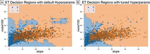
Figure 6 shows an instance of ET decision regions pre- and post-optimisation by finding the best combination of hyperparameter values to minimise both variance and bias. The pre-optimisation decision regions (Figure 6a) highlight some overfitting represented by small regions that split only a few isolated samples of one class embedded in the other. Those erroneous regions suggest overfitting and need to be removed to allow the model to better generalise to new data. Among other hyperparams (e.g. max depth, number of estimators, etc.), the tuned ET model was set to not split below a minimum number of samples, thus removing those isolated regions as shown in Figure 6(b).

Figure 6. Decision regions between slope angle and relative relief computed by the ExtraTreesClassifier before (A) and after (B) the optimisation process achieved with hyperparameters tuning, which returned optimal parameter values, including number of trees, minimum number of samples to split and maximum depth equal to 60, 2 and 25 respectively.

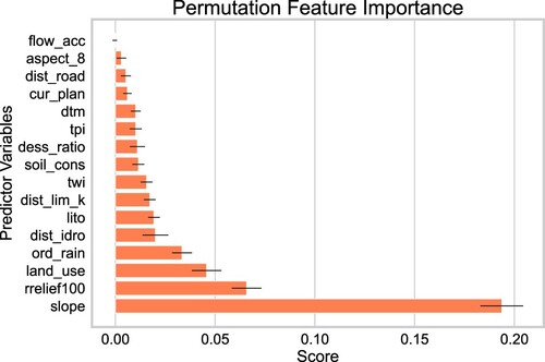
To understand how the model works, the importance of each variable was sorted from the most to least predictive (Figure 7). The higher the slope and relative relief the higher the landslide susceptibility, as also shown by the decision regions plot. Land use results as the third most important variable. Ordinary annual rainfall, distance to streams, litho-technical units, distance to permeability limits as well as TWI follow respectively. It should be noted the high consistency of variable importance given the slight standard deviation displayed. Permutation features importance results also denote the positive contribution of almost all the predictor variables to model performance, thus indicating that the selected variables should be kept. Flow accumulation is the only feature that appears irrelevant to the model.

Figure 7. Average permutation feature importance with standard deviations derived by repeating the shuffling process 15 times.

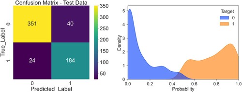
To represent the ability of the model to generalise to never seen data, the confusion matrix together with kernel density of probabilities (Figure 8) have been computed on the 20% of the data we held before creating the model (i.e. out-of-sample test set). The tabular confusion matrix denotes the number of predictions made by the model where it classified the classes correctly or incorrectly. Using a probability threshold of 0.5, we have almost 90% of correctly classified data for both 0s (i.e. stable points) and 1s (i.e. LIP). The reliability of the model is also certified by the overall precision, recall and F1-score which have values of 0.88 or 0.89. The kernel density plot represents the distribution of predicted probabilities for the withheld test data. This plot suggests a strong separation between LIP samples and stable point data. LIP samples are almost never getting a probability below 0.4. The median probabilities stand close to 0 and 0.9 for stable and LIP samples respectively (Figure 8).

Figure 8. Confusion matrix plot (left) and classification report (right) of predicted labels for the test dataset. Kernel density plot of predicted probabilities for the test samples.

The resulting prediction across the whole mapped extent and some example areas at a larger scale is provided in Figure 9. Red areas are those that are predicted to have a high likelihood of slope failure occurrence while green areas are predicted as having a low likelihood.

Figure 9. Urban-scale landslide susceptibility of Rome (namely URGENT Rome) derived with the tuned Extra Trees Classifier (left). A detailed example of Monte Mario hill with superimposed the event-based test samples (right).

4.2. Multiscale LSZ reliability assessment

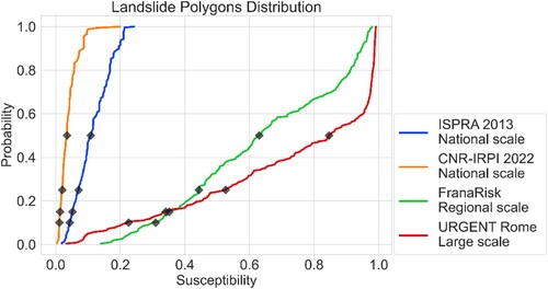
Figure 10 shows the empirical cumulative distribution of susceptibility values in the overall landslide polygons for each quantitative LSZ. The distributions appear significantly different among all scales of analysis. The national scale maps (i.e. ISPRA 2013 and CNR-IRPI 2022) have a totality of values below 0.2. It should be noted that the distribution of URGENT Rome predictions is typically greater than the others, with FranaRisk close behind. The FranaRisk LSZ performs better than others until the 15th percentile and then decreases with respect to the URGENT Rome values.

Figure 10. ECDF of mean susceptibilities predicted to landslides stored in the database as polygons. Black dots represent the percentile thresholds employed to derive the five classes.

Once reclassified, similarity analysis of the pair of LSZ for the event-based test samples LIP (Figure 11) and the overall landslide polygons (Figure 12) allowed us to compute a mean distance in susceptibility class distribution between the existing maps and URGENT Rome LSZ (i.e. the Wasserstein distance). Regarding the event-based test samples, the NASA Global LSZ as well as the ELSUSv2 Pan-European map are the furthest from URGENT Rome with an average distance of 1.84 and 1.82 classes respectively. CNR-IRPI 2022 and ISPRA 2013 maps gained much more predictive capacity as reported by the Wasserstein distance results of 0.33 and 1.12. FranaRisk confirms to be the closest to URGENT Rome with only 0.12 classes of distance.

Figure 11. Wasserstein distance as the area between cumulative distributions of 2014 event-based LIPs as predicted by LSZ. The Wasserstein Distance of categorical features expresses the difference in landslide susceptibility classes between the tested map and the benchmark (i.e. URGENT Rome).

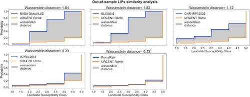
Figure 12. Wasserstein distance as the area between cumulative distributions of the overall landslides as predicted by LSZ. The Wasserstein Distance of categorical features expresses the difference in landslide susceptibility classes between the tested map and the benchmark (i.e. URGENT Rome).

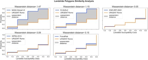
As regards landslide polygons, the NASA Global LS map and ELSUSv2 still remain the furthest, while ISPRA 2013 and CNR-IRPI 2022 got even closer than FranaRisk, with the CNR-IRPI 2022 being almost identical (0.05 classes).

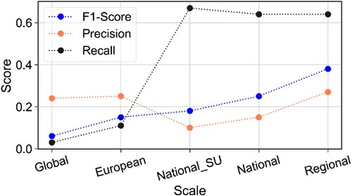
Spatialised accuracy assessment confirms the low capacity of LSZ at European and global scales to detect true landslides since 97% and 89% of false negatives were recorded by NASA LSZ and ELSUSv2 respectively (Figure 13). The national scale LSZ (i.e. ISPRA 2013 and CNR-IRPI 2022) improves the ability to detect true landslides. However, they report a high landslide susceptibility level even in areas not prone to landslides (i.e. false positives). Whereas FranaRisk LSZ keeps the predictive capabilities for true landslides but improves the detection of true negatives compared to the nationwide maps. As a result, the spatial accuracy assessment returned scoring metrics (e.g. F1-score) that increase proportionally with the scale of the LSZ (Figure 14).

Figure 13. Spatialised performance assessment of each open-source LSZ with reference to URGENT Rome LSZ.

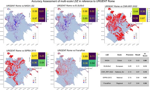
Figure 14. Line plot of evaluation metrics obtained from the spatialised accuracy assessment of open-source LSZ at different scales of investigation.

Performance metrics relative to original and merged LS maps (both cumulative and pairwise) are summarised in Figure 15. Precision scores (Figure 15c) highlight low performance of all the considered maps. Among the others, the original LSZ at regional scale (i.e. FranaRisk) stands as the closer to the reference, and it is closely followed by its integration with the national scale map (i.e. ISPRA 2013). Eventually, precision values of multiscale maps remain close to the original ones.

Figure 15. Comparison of F1-score (a), Recall (b) and Precision (c) scores for both original and multiscale landslide susceptibility maps with reference to URGENT Rome LSZ.

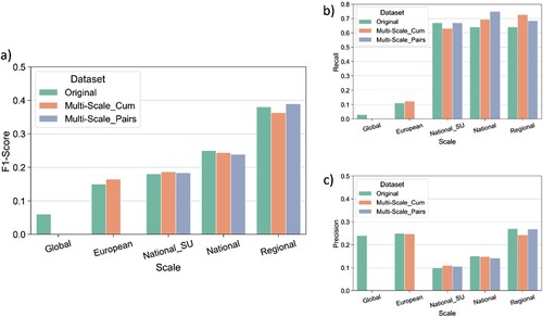
On the other hand, recall scores (Figure 15b) are always higher than original maps, with the fusion of the two nationwide maps (i.e. ISPRA 2013 and CNR-IRPI 2022) producing the highest performance (0.75). Anyway, the cumulative fusion of all LSZ is only 0.02 away.

By bringing together recall and precision, the resulting F1 scores (Figure 15a) provided an overall picture of the performance. As a result, the map that comes closest to URGENT Rome LSZ is provided by the fusion of FranaRisk and ISPRA 2013 maps (F1-score of 0.39), improving the performance of the best original map.

5. Discussion

The several supervised machine learning classifiers individually trained and validated by means of the K-fold cross validation technique allowed us to identify the ET model as the best performing one among others. Generally, all the trained models perform well, but the ET outperforms the others in any calculated metric. We stress the importance of model optimisation by tuning its hyperparameters, thus finding the optimal minimum between bias and variance. Moreover, tree-based models have a strong tendency to overestimate the importance of continuous numerical or high cardinality categorical features because they provide more opportunity for the models to split the data in half than the discrete features. Therefore, the default feature importance function of tree-based models returns biased results. Indeed, to overcome this problem we recommend using the permutation feature importance method, which also lists the features that worsen the model performance. In urban areas like the city of Rome, morphological variables such as slope angle and relative relief play the most important role in the prediction of the landslide susceptibility value, which is consistent with previous studies (Baeza, Lantada, and Amorim 2016; Maxwell et al. 2020; Titti et al. 2022). This is probably due to urbanisation activities which generate man-made steep slopes close to the almost flat urban network. Nevertheless, cumulated annual rainfall, land use and litho-technical units play an important role as preparatory and predisposing factors for shallow landslides.

The final optimised model tested with the held 20% of the samples correctly classified almost 90% of both positive and negative samples, thus confirming its generalisation capabilities and allowing its deployment to predict landslide susceptibility for the whole area of the Municipality of Rome. Indeed, incorrectly classified samples never get susceptibility further than 0.1 from the binary classification threshold (i.e. 0.5).

The urban-scale LS map (i.e. URGENT Rome) highlights the hotspots of Monte Mario and Monte Ciocci hills. This was indeed confirmed by considering the event-based test samples related to the landslides of January 2014 that occurred mostly along the south-eastern slope of the hill. We stress that the rainfall-triggered landslides in winter 2014 represent an out-of-sample set that the model has never seen. Other high susceptibility areas are represented by steep slopes near the streams, especially in the northern sector of the municipality, where volcanic deposits have been strongly eroded.

Once obtained the urban-scale URGENT Rome LSZ has been compared to other available open-source LSZ built at different scales of investigation. Firstly, we applied the empirical cumulative distribution function to reclassify quantitative maps in 5 hazard classes. This allowed us to make them comparable with the already qualitative maps (i.e. NASA and ELSUSv2 LSZ). Since the ECDF curve shows the probability of local landslides to be predicted, we stress that this reclassification method may strongly increase the predictive performance of hazard products made at small and medium scales. However, percentiles values to be used as class thresholds are not standardised and they rely on expert judgment. This is proved by the similarity analysis, in which the national scale maps show reduced differences with the URGENT Rome LSZ. The similarity analysis carried out on both 2014 event-based LIPs and landslide polygons highlighted the effect of mapping unit as well as pixel size, and therefore the overall scale of analysis. Among the maps that were compared, grid-based ones perform better when predicting landslide initiation points, and the larger the scale the closest the map with respect to the reference. The SU-based LSZ turns out to be the closest to URGENT Rome when predicting the entire area potentially affected. This is because it assigns a uniform hazard level to the whole slope. Although the similarity analysis carried out with the Wasserstein distance metric concerns true positives only, the ability of hazard products to detect stable areas (i.e. true negatives) must be also evaluated. With this purpose, we carried out a spatialised accuracy assessment which returned the number of true/false positives and true/false negatives throughout the map. The results confirm the low capacity of global and European scale maps to detect true landslides, thus resulting in a significant underestimation of landslide hazard in Rome. As suggested by the similarity analysis, national scale maps may be adequate to detect areas susceptible to landsliding, but they overestimate them, thus resulting in high false positive rates (i.e. low precision). The regional scale map has the most high and balanced scores. It’s worth noting that landslide inventory is partially overlapped with the one considered in URGENT urban susceptibility zoning. Although it has the biggest F1-score, it is still far from URGENT Rome. According to Cascini (2008) and Corominas et al. (2013), the larger the scale the most reliable the zoning is, thus changing its purposes. Hereby, we spotted the linear increment of F1-scores with the scale of analysis. We stress that this is probably due to the resolution and distribution of input data which inevitably are biased and incomplete when very large areas must be considered. Landslide hazard assessment at a large or detailed scale is often lacking. However, the proposed method for merging a variety of low accuracy products represents an attempt to improve the predictive performance of the single ones and gaining reliability. The several LSZ were integrated cumulatively and pairwise to evaluate the accuracy at each integration. The closest reliability and classification scores can be achieved by merging the FranaRisk and ISPRA 2013 maps (i.e. regional, and national scale). Despite a general limited improvement reached by merging the multiple scale maps, the implemented method can enhance the proportion of actual landslides correctly classified (i.e. the recall metric). With this perspective, the adopted data fusion criteria increased the ability to detect occurred landslides while maintaining precision. However, the number of false positives remains high as for original maps, thus affecting the overall F1 scores.

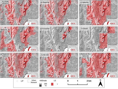
As an example, Figure 16 shows how the Monte Mario hill is classified by the different LS maps. In contrast to URGENT Rome (Figure 16a), the fusion of lower resolution original LSZ (Figure 16g–i), although they properly classify all LIPs, also misclassify some terrains surrounding the slopes that may not be prone to landslide. This reflects on the number of buildings that would be exposed to landslide risk within the municipality. In fact, it goes from a truthful 3% of the urban-scale URGENT Rome map up to about 25% recorded with the fusion of the two nationwide maps. With this perspective, site-specific urban scale landslide susceptibility analyses are always required for a balanced assessment of landslide hazard when detailed risk analysis and/or land-use planning are carried out.

Figure 16. Details of predicted landslide susceptibility at the Monte Mario hill and overall percentage of exposed buildings within the municipality of Rome according to each product. The URGENT Rome map (a) compared with the original open-source LS products built at different scales of analysis (b – f) and with the top performing products obtained with the fusion criteria: regional and national scale (b), all available maps (c) and the two nationwide maps based on different mapping unit (d). Landslide Initiation Points (LIP) and the Roman urban network are plotted on each map.

6. Conclusion

This study reports the complete and comprehensive workflow that should be implemented to obtain urban-scale LS maps when dealing with data-driven methods as supervised machine learning (ML) algorithms. Thorough pre-processing stages are fundamental to prepare data for machine learning. In this research, we tested various ML models to select the optimal and most performing one for landslide and stability classification in the urban area of Rome (Italy). Through empirical cumulative distribution functions applied to the out-of-samples landslides we selected susceptibility class thresholds based on model performance to correctly classify landslides. Once validated, the largest scale LSZ available in Rome was compared with regional, national, European and global scale LS products.

ECDF were used to standardise the reclassification of continuous LS maps once values of percentiles are determined. Comparisons between LSZ reveal differences in the ability to predict instability and stability with respect to the reference. The main outcomes revealed how the pixel size as well as the adopted mapping unit play a crucial role in the result. Specifically, wide grids fail to accurately localise potential landslide and stable areas. Whereas LSZ based on slope unit may give comprehensive information about the overall area potentially affected by the landslide evolution, they do not allow the direct definition of the source areas, which can be improved by merging grid and SU-based products. The implemented multiscale zoning method assigns a specific accuracy value to individual maps, which is appropriately accounted for when merging.

In a general perspective, the fusion of multiple low-resolution maps increased the ability to correctly classify occurred landslides; however, with the adopted method, the improvement in general performance is not enough to justify its deployment due to the high number of false positives. Nevertheless, when both urban and regional scale products are lacking, the fusion of national, European and global maps might significantly help in better predict landslides occurrence in urban areas.

Disclosure statement

No potential conflict of interest was reported by the author(s).

Data availability statement

We share the necessary data to make our study transparent and reproducible. The landslide database and the urban-scale landslide susceptibility map of Rome reported in this work are available at the following repository: 10.5281/zenodo.7589881.

Additional information

Funding

This research is framed within the PRIN 2017 project – URGENT “URban Geology and geohazards: Engineering geology for safer, resilieNt and smart ciTies” – UR SAPIENZA.

References

- Alessi, Dario, Francesca Bozzano, Andrea Lisa, Carlo Esposito, Andrea Fantini, Adriano Loffredo, Salvatore Martino, et al. 2014. “Geological Risks in Large Cities: The Landslides Triggered in the City of Rome (Italy) by the Rainfall of 31 January-2 February 2014.” Italian Journal of Engineering Geology and Environment 1 (June): 15–34. doi:10.4408/IJEGE.2014-01.O-02.
- Ali, Moez. 2020. “PyCaret: An Open Source, Low-Code Machine Learning Library in Python.” PyCaret Version 2.
- Altmann, André, Laura Toloşi, Oliver Sander, and Thomas Lengauer. 2010. “Permutation Importance: A Corrected Feature Importance Measure.” Bioinformatics (Oxford, England) 26 (10): 1340–1347. https://doi.org/10.1093/bioinformatics/btq134.
- Alvioli, Massimiliano, Fausto Guzzetti, and Ivan Marchesini. 2020. “Parameter-Free Delineation of Slope Units and Terrain Subdivision of Italy.” Geomorphology 358 (June): 107124. https://doi.org/10.1016/j.geomorph.2020.107124.
- Amanti, M., V. Chiessi, and P. M. Guarino. 2012. “The 13 November 2007 Rock-Fall at Viale Tiziano in Rome (Italy).” Natural Hazards and Earth System Sciences 12 (5): 1621–1632. https://doi.org/10.5194/nhess-12-1621-2012. Copernicus GmbH.
- Argentieri, A., C. Esposito, M. Fabiani, G. M. Marmoni, M. Piro, G. Rotella, G. Scarascia Mugnozza, and P. Vitali. 2018. “The “Franarisk” Project in Rome Metropolitan Area: A Tool for Land Planning and Management and for Preliminary Risk Assessment of Infrastructures and Buildings.” In Catania, SGI-SIMP 2018.
- Baeza, Cristina, and Jordi Corominas. 2001. “Assessment of Shallow Landslide Susceptibility by Means of Multivariate Statistical Techniques.” Earth Surface Processes and Landforms 26 (12): 1251–1263. https://doi.org/10.1002/esp.263.
- Baeza, Cristina, Nieves Lantada, and Samuel Amorim. 2016. “Statistical and Spatial Analysis of Landslide Susceptibility Maps with Different Classification Systems.” Environmental Earth Sciences 75 (19): 1318. https://doi.org/10.1007/s12665-016-6124-1.
- Basu, Tirthankar, and Swades Pal. 2018. “Identification of Landslide Susceptibility Zones in Gish River Basin, West Bengal, India.” Georisk: Assessment and Management of Risk for Engineered Systems and Geohazards 12 (1): 14–28. https://doi.org/10.1080/17499518.2017.1343482. Taylor & Francis.
- Bhuyan, Kushanav, Hakan Tanyaş, Lorenzo Nava, Silvia Puliero, Sansar Raj Meena, Mario Floris, Cees van Westen, and Filippo Catani. 2023. “Generating Multi-Temporal Landslide Inventories Through a General Deep Transfer Learning Strategy Using HR EO Data.” Scientific Reports 13 (1): 162. https://doi.org/10.1038/s41598-022-27352-y. Nature Publishing Group.
- Bordoni, M., V. Vivaldi, L. Lucchelli, L. Ciabatta, L. Brocca, J. P. Galve, and C. Meisina. 2021. “Development of a Data-Driven Model for Spatial and Temporal Shallow Landslide Probability of Occurrence at Catchment Scale.” Landslides 18 (4): 1209–1229. https://doi.org/10.1007/s10346-020-01592-3.
- Bozzano, F., A. Andreucci, M. Gaeta, and R. Salucci. 2000. “A Geological Model of the Buried Tiber River Valley Beneath the Historical Centre of Rome.” Bulletin of Engineering Geology and the Environment 59 (1): 1–21. https://doi.org/10.1007/s100640000051.
- Bozzano, Francesca, Carlo Esposito, Stefania Franchi, Paolo Mazzanti, Daniele Perissin, Alfredo Rocca, and Emanuele Romano. 2015. “Analysis of a Subsidence Process by Integrating Geological and Hydrogeological Modelling with Satellite InSAR Data.” In Engineering Geology for Society and Territory - Volume 5, edited by Giorgio Lollino, Andrea Manconi, Fausto Guzzetti, Martin Culshaw, Peter Bobrowsky, and Fabio Luino, 155–159. Cham: Springer International Publishing. https://doi.org/10.1007/978-3-319-09048-1_31.
- Brabb, Earl E. 1984. Innovative Approaches to Landslide Hazard and Risk Mapping. Proceedings of the 4th international symposium on landslides, Toronto, Canada, 1, 30–32.
- Cascini, Leonardo. 2008. “Applicability of Landslide Susceptibility and Hazard Zoning at Different Scales.” Engineering Geology 102 (3-4): 164–177. https://doi.org/10.1016/j.enggeo.2008.03.016.
- Ciotoli, Giancarlo, E. Loreto, Lorenzo Liperi, Fabio Meloni, Stefania Nisio, and Adelaide Sericola. 2014. Carta Dei Sinkhole Naturali Del Lazio 2012 e Sviluppo Futuro Del Progetto Sinkholes Regione Lazio’.
- Corominas, J., C. van Westen, P. Frattini, L. Cascini, J.-P. Malet, S. Fotopoulou, F. Catani, et al. 2013. “Recommendations for the Quantitative Analysis of Landslide Risk.” Bulletin of Engineering Geology and the Environment 73 (2): 209–263. https://doi.org/10.1007/s10064-013-0538-8.
- Crosta, G. B., S. Imposimato, D. Roddeman, S. Chiesa, and F. Moia. 2005. “Small Fast-Moving Flow-Like Landslides in Volcanic Deposits: The 2001 Las Colinas Landslide (El Salvador).” Engineering Geology 79 (3-4): 185–214. https://doi.org/10.1016/j.enggeo.2005.01.014.
- Cui, Yifei, Deqiang Cheng, Clarence E. Choi, Wen Jin, Yu Lei, and Jeffrey S. Kargel. 2019. “The Cost of Rapid and Haphazard Urbanization: Lessons Learned from the Freetown Landslide Disaster.” Landslides 16 (6): 1167–1176. https://doi.org/10.1007/s10346-019-01167-x.
- Del Monte, Maurizio, Maurizio D’Orefice, Gian Marco Luberti, Roberta Marini, Alessia Pica, and Francesca Vergari. 2016. “Geomorphological Classification of Urban Landscapes: The Case Study of Rome (Italy).” Journal of Maps 12 (sup1): 178–189. https://doi.org/10.1080/17445647.2016.1187977. Taylor & Francis.
- Esposito, Carlo, Niccolò Belcecchi, Francesca Bozzano, Alessandro Brunetti, Gian Marco Marmoni, Paolo Mazzanti, Saverio Romeo, Flavio Cammillozzi, Giancarlo Cecchini, and Massimo Spizzirri. 2021. “Integration of Satellite-Based A-DInSAR and Geological Modeling Supporting the Prevention from Anthropogenic Sinkholes: A Case Study in the Urban Area of Rome.” Geomatics, Natural Hazards and Risk 12 (1): 2835–2864. https://doi.org/10.1080/19475705.2021.1978562. Taylor & Francis.
- Esposito, Carlo, Giandomenico Mastrantoni, Gian Marco Marmoni, Benedetta Antonelli, Patrizia Caprari, Alessia Pica, Luca Schilirò, and Francesca Bozzano. 2023. “From theory to practice: optimisation of available information for landslide hazard assessment in Rome relying on official, fragmented data sources.” Landslides. https://doi.org/10.1007/s10346-023-02095-7.
- Fawcett, Tom. 2006. “An Introduction to ROC Analysis.” Pattern Recognition Letters, ROC Analysis in Pattern Recognition 27 (8): 861–874. https://doi.org/10.1016/j.patrec.2005.10.010.
- Fell, Robin, Jordi Corominas, Christophe Bonnard, Leonardo Cascini, Eric Leroi, and William Z. Savage. 2008. “Guidelines for Landslide Susceptibility, Hazard and Risk Zoning for Land-Use Planning.” Engineering Geology 102 (3-4): 99–111. https://doi.org/10.1016/j.enggeo.2008.03.014.
- Flentje, Phillip N, Anthony Miner, Graham Whitt, and Robin Fell. 2007. “Guidelines for Landslide Susceptibility.” Hazard and Risk Zoning for Land Use Planning’ 42 (1): 28.
- Funiciello, R., and G. Giordano. 2008. “The Geological Map of Rome: Lithostratigraphy and Stratigraphic Organization.” La Geologia Di Roma. Dal Centro Storico Alla Periferia II. Mem Desc Carta Geologica D’Italia 80:39–85.
- Günther, Andreas, Miet Van Den Eeckhaut, Jean-Philippe Malet, Paola Reichenbach, and Javier Hervás. 2014. “Climate-Physiographically Differentiated Pan-European Landslide Susceptibility Assessment Using Spatial Multi-Criteria Evaluation and Transnational Landslide Information.” Geomorphology 224 (November): 69–85. https://doi.org/10.1016/j.geomorph.2014.07.011.
- Guzzetti, Fausto, Alberto Carrara, Mauro Cardinali, and Paola Reichenbach. 1999. “Landslide Hazard Evaluation: A Review of Current Techniques and Their Application in a Multi-Scale Study, Central Italy.” Geomorphology 31 (1-4): 181–216. https://doi.org/10.1016/S0169-555X(99)00078-1.
- Hungr, Oldrich, Serge Leroueil, and Luciano Picarelli. 2014. “The Varnes Classification of Landslide Types, an Update.” Landslides 11 (2): 167–194. https://doi.org/10.1007/s10346-013-0436-y.
- Hutchinson, Michael F., Tingbao Xu, and John A. Stein. 2011. “Recent Progress in the ANUDEM Elevation Gridding Procedure.” Geomorphometry 2011:19–22. International Society for Geomorphometry Redlands.
- Iadanza Carla, Carlo Cacace, Sara Del Conte, Daniele Spizzichino, Stefano Cespa & Alessandro Trigila. 2013. ‘Cultural Heritage, Landslide Risk and Remote Sensing in Italy’. In Landslide Science and Practice: Volume 6: Risk Assessment, Management and Mitigation, edited by Claudio Margottini, Paolo Canuti, and Kyoji Sassa, 491–499. Berlin, Heidelberg: Springer. https://doi.org/10.1007/978-3-642-31319-6_65.
- Iadanza, C., A. Trigila, P. Starace, A. Dragoni, T. Biondo, and M. Roccisano. 2021. “IdroGEO: A Collaborative Web Mapping Application Based on REST API Services and Open Data on Landslides and Floods in Italy.” ISPRS International Journal of Geo-Information 10 (2): 89. https://doi.org/10.3390/ijgi10020089. Multidisciplinary Digital Publishing Institute.
- Iadanza, C., A. Trigila, E. Vittori, and L. Serva. 2009. “Landslides in Coastal Areas of Italy.” Geological Society, London, Special Publications 322 (1): 121–141. https://doi.org/10.1144/SP322.5. Geological Society of London.
- Jurgiel, Borys. 2013. “Borysiasty/Pointsamplingtool.” Python. https://github.com/borysiasty/pointsamplingtool.
- Kainthura, Poonam, and Neelam Sharma. 2022. “Machine Learning Driven Landslide Susceptibility Prediction for the Uttarkashi Region of Uttarakhand in India.” Georisk: Assessment and Management of Risk for Engineered Systems and Geohazards 16 (3): 570–583. https://doi.org/10.1080/17499518.2021.1957484. Taylor & Francis.
- Kiersch, G. 1964. “Vaiont Reservoir Disaster.” Civil Engineering, ASCE 34: 32–47.
- Kotsiantis, Sotiris B., Dimitris Kanellopoulos, and Panagiotis E. Pintelas. 2006. “Data Preprocessing for Supervised Leaning.” International Journal of Computer Science 1 (2): 111–117. Citeseer.
- Kuhn, Max, and Kjell Johnson. 2013. Applied Predictive Modeling. New York, NY: Springer.
- La Vigna, Francesco, Roberto Mazza, Marco Amanti, Cristina Di Salvo, Marco Petitta, and Luca Pizzino. 2015. “The Synthesis of Decades of Groundwater Knowledge: The New Hydrogeological Map of Rome.” Acque Sotterranee - Italian Journal of Groundwater 4 (4): 9–17. https://doi.org/10.7343/as-128-15-0155.
- Loche, Marco, Massimiliano Alvioli, Ivan Marchesini, Haakon Bakka, and Luigi Lombardo. 2022. Landslide Susceptibility Maps of Italy: Lesson Learnt from Dealing with Multiple Landslide Classes and the Uneven Spatial Distribution of the National Inventory. Preprint. Physical Sciences and Mathematics. https://doi.org/10.31223/X5Q92S.
- Luberti, Gian Marco, Francesca Vergari, Roberta Marini, Alessia Pica, and Maurizio Del Monte. 2018. “Anthropogenic Modifications to the Drainage Network of Rome (Italy): The Case Study of the Aqua Mariana.” Alpine and Mediterranean Quaternary 31 (2): 119–132. https://doi.org/10.26382/AMQ.2018.08.
- Luo, Junyao, Lulu Zhang, Haoqing Yang, Xin Wei, Dongsheng Liu, and Jiabao Xu. 2022. “Probabilistic Model Calibration of Spatial Variability for a Physically-Based Landslide Susceptibility Model.” Georisk: Assessment and Management of Risk for Engineered Systems and Geohazards 16 (4): 728–745. https://doi.org/10.1080/17499518.2021.1988986. Taylor & Francis.
- Martino, S., F. Bozzano, P. Caporossi, D. D’Angiò, M. Della Seta, C. Esposito, A. Fantini, et al. 2019. “Impact of Landslides on Transportation Routes During the 2016–2017 Central Italy Seismic Sequence.” Landslides 16 (6): 1221–1241. https://doi.org/10.1007/s10346-019-01162-2.
- Mastrantoni, Giandomenico, Patrizia Caprari, Carlo Esposito, Gian Marco Marmoni, Paolo Mazzanti, and Francesca Bozzano. 2022. Data Requirements and Scientific Efforts for Reliable Large-Scale Assessment of Landslide Hazard in Urban Areas. EGU22-4669. Copernicus Meetings. https://doi.org/10.5194/egusphere-egu22-4669.
- Mateos, Rosa María, Juan López-Vinielles, Eleftheria Poyiadji, Dimetrios Tsagkas, Michael Sheehy, Kleopas Hadjicharalambous, Pavel Liscák, et al. 2020. “Integration of Landslide Hazard Into Urban Planning Across Europe.” Landscape and Urban Planning 196 (April): 103740. https://doi.org/10.1016/j.landurbplan.2019.103740.
- Maxwell, Aaron E., Maneesh Sharma, James S. Kite, Kurt A. Donaldson, James A. Thompson, Matthew L. Bell, and Shannon M. Maynard. 2020. “Slope Failure Prediction Using Random Forest Machine Learning and LiDAR in an Eroded Folded Mountain Belt.” Remote Sensing 12 (3): 486. https://doi.org/10.3390/rs12030486. Multidisciplinary Digital Publishing Institute.
- Mazzanti, P., and F. Bozzano. 2011. “Revisiting the February 6th 1783 Scilla (Calabria, Italy) Landslide and Tsunami by Numerical Simulation.” Marine Geophysical Research 32 (1-2): 273–286. https://doi.org/10.1007/s11001-011-9117-1.
- Ngadisih, Ryuichi Yatabe, Netra P. Bhandary, and Ranjan K. Dahal. 2014. “Integration of Statistical and Heuristic Approaches for Landslide Risk Analysis: A Case of Volcanic Mountains in West Java Province, Indonesia.” Georisk: Assessment and Management of Risk for Engineered Systems and Geohazards 8 (1): 29–47. https://doi.org/10.1080/17499518.2013.826030. Taylor & Francis.
- Oguchi, Takashi. 1997. “Drainage Density and Relative Relief in Humid Steep Mountains with Frequent Slope Failure.” Earth Surface Processes and Landforms 22 (2): 107–120. https://doi.org/10.1002/(SICI)1096-9837(199702)22:2<107::AID-ESP680>3.0.CO;2-U.
- Parotto, M. 2008. “Evoluzione Paleogeografica Dell’area Romana: Una Breve Sintesi.’ Special Volume “La Geologia di Roma. Dal Centro Storico Alla Periferia”.” Memorie Descrittive Della Carta Geologica D’Italia 80: 25–38.
- Pedregosa, Fabian, Gael Varoquaux, Alexandre Gramfort, Vincent Michel, Bertrand Thirion, Olivier Grisel, Mathieu Blondel, et al. 2011. “Scikit-Learn: Machine Learning in Python.” Machine Learning in Python 12: 2825–2830.
- Persichillo, Maria Giuseppina, Massimiliano Bordoni, Claudia Meisina, Carlotta Bartelletti, Michele Barsanti, Roberto Giannecchini, Giacomo D’Amato Avanzi, et al. 2017. “Shallow Landslides Susceptibility Assessment in Different Environments.” Geomatics, Natural Hazards and Risk 8 (2): 748–771. https://doi.org/10.1080/19475705.2016.1265011. Taylor & Francis.
- Piccoli, Benedetto, and Francesco Rossi. 2016. “On Properties of the Generalized Wasserstein Distance.” Archive for Rational Mechanics and Analysis 222 (3): 1339–1365. https://doi.org/10.1007/s00205-016-1026-7. Springer.
- Reichenbach, Paola, Mauro Rossi, Bruce D. Malamud, Monika Mihir, and Fausto Guzzetti. 2018. “A Review of Statistically-Based Landslide Susceptibility Models.” Earth-Science Reviews 180 (May): 60–91. https://doi.org/10.1016/j.earscirev.2018.03.001.
- Salvati, P., C. Bianchi, M. Rossi, and F. Guzzetti. 2010. “Societal Landslide and Flood Risk in Italy.” Natural Hazards and Earth System Sciences 10 (3): 465–483. https://doi.org/10.5194/nhess-10-465-2010. Copernicus GmbH.
- Saulnier, Georges-Marie, Keith Beven, and Charles Obled. 1997. “Including Spatially Variable Effective Soil Depths in TOPMODEL.” Journal of Hydrology 202 (1-4): 158–172. https://doi.org/10.1016/S0022-1694(97)00059-0.
- Schilirò, L., G. Poueme Djueyep, C. Esposito, and G. Scarascia Mugnozza. 2019. “The Role of Initial Soil Conditions in Shallow Landslide Triggering: Insights from Physically Based Approaches.” Geofluids 2019 (June): e2453786. https://doi.org/10.1155/2019/2453786. Hindawi.
- Soeters, Robert, and C. J. Van Westen. 1996. “Slope Instability Recognition, Analysis and Zonation.” In Landslides: Investigation and Mitigation 247, edited by A. Keith Turner and Robert L. Schuster, 129–177. Washington, DC: National Academy Press.
- Stanley, Thomas, and Dalia B. Kirschbaum. 2017. “A Heuristic Approach to Global Landslide Susceptibility Mapping.” Natural Hazards 87 (1): 145–164. https://doi.org/10.1007/s11069-017-2757-y.
- Su, Chenxu, Bijiao Wang, Yunhong Lv, Mingpeng Zhang, Dalei Peng, Bate Bate, and Shuai Zhang. 2022. “Improved Landslide Susceptibility Mapping Using Unsupervised and Supervised Collaborative Machine Learning Models.” Georisk: Assessment and Management of Risk for Engineered Systems and Geohazards 0 (0): 1–19. https://doi.org/10.1080/17499518.2022.2088802. Taylor & Francis.
- Titti, Giacomo, Alessandro Sarretta, Luigi Lombardo, Stefano Crema, Alessandro Pasuto, and Lisa Borgatti. 2022. “Mapping Susceptibility With Open-Source Tools: A New Plugin for QGIS.” Frontiers in Earth Science 10 (March): 842425. https://doi.org/10.3389/feart.2022.842425.
- Tonini, M., G. Pecoraro, K. Romailler, and M. Calvello. 2022. “Spatio-Temporal Cluster Analysis of Recent Italian Landslides.” Georisk: Assessment and Management of Risk for Engineered Systems and Geohazards 16 (3): 536–554. https://doi.org/10.1080/17499518.2020.1861634. Taylor & Francis.
- Trigila, Alessandro, Paolo Frattini, Nicola Casagli, Filippo Catani, Giovanni Crosta, Carlo Esposito, Carla Iadanza, et al. 2013. “Landslide Susceptibility Mapping at National Scale: The Italian Case Study.” In Landslide Science and Practice: Volume 1: Landslide Inventory and Susceptibility and Hazard Zoning, edited by Claudio Margottini, Paolo Canuti, and Kyoji Sassa, 287–295. Berlin, Heidelberg: Springer. https://doi.org/10.1007/978-3-642-31325-7_38.
- Trigila, Alessandro, Carla Iadanza, Carlo Esposito, and Gabriele Scarascia-Mugnozza. 2015. “Comparison of Logistic Regression and Random Forests Techniques for Shallow Landslide Susceptibility Assessment in Giampilieri (NE Sicily, Italy).” Geomorphology, Geohazard Databases: Concepts, Development, Applications 249 (November): 119–136. https://doi.org/10.1016/j.geomorph.2015.06.001.
- Trigila, Alessandro, Carla Iadanza, Michele Munafò, and Ines Marinosci. 2015. “Population Exposed to Landslide and Flood Risk in Italy.” In Engineering Geology for Society and Territory - Volume 5, edited by Giorgio Lollino, Andrea Manconi, Fausto Guzzetti, Martin Culshaw, Peter Bobrowsky, and Fabio Luino, 843–848. Cham: Springer International Publishing. https://doi.org/10.1007/978-3-319-09048-1_163.
- Trigila, Alessandro, Carla Iadanza, and Daniele Spizzichino. 2010. “Quality Assessment of the Italian Landslide Inventory Using GIS Processing.” Landslides 7 (4): 455–470. https://doi.org/10.1007/s10346-010-0213-0.
- van Westen, Cees J., Enrique Castellanos, and Sekhar L. Kuriakose. 2008. “Spatial Data for Landslide Susceptibility, Hazard, and Vulnerability Assessment: An Overview.” Engineering Geology, Landslide Susceptibility, Hazard and Risk Zoning for Land Use Planning 102 (3): 112–131. https://doi.org/10.1016/j.enggeo.2008.03.010.
- Vijith, H., K. N. Krishnakumar, G. S. Pradeep, M. V. Ninu Krishnan, and G. Madhu. 2014. “Shallow Landslide Initiation Susceptibility Mapping by GIS-Based Weights-of-Evidence Analysis of Multi-Class Spatial Data-Sets: A Case Study from the Natural Sloping Terrain of Western Ghats, India.” Georisk: Assessment and Management of Risk for Engineered Systems and Geohazards 8 (1): 48–62. https://doi.org/10.1080/17499518.2013.843437. Taylor & Francis.
- Wilde, Martina, Andreas Günther, Paola Reichenbach, Jean-Philippe Malet, and Javier Hervás. 2018. “Pan-European Landslide Susceptibility Mapping: ELSUS Version 2.” Journal of Maps 14 (2): 97–104. https://doi.org/10.1080/17445647.2018.1432511.