On the use of different data assimilation schemes in a fully coupled hydro-mechanical slope stability analysis

ABSTRACT

Different data assimilation schemes such as the ensemble Kalman filter (EnKF), ensemble smoother (ES) and ensemble smoother with multiple data assimilation (ESMDA) are implemented in a hydro-mechanical slope stability analysis. For a synthetic case, these schemes assimilate displacements at the crest and the slope to estimate strength and stiffness parameters. These estimated parameters are then used to estimate the system's state and factor of safety (FoS). The results show that EnKF provides an FoS estimation with a mean close to the truth and with the smallest standard deviation, with ESMDA using the largest amount of assimilation steps also providing a mean close to the truth but with less confidence. The ES and ESMDA with fewer assimilation steps underestimate the FoS approximation and have low confidence. Assimilating measurements over a longer period provides a more accurate parameter, state and FoS estimation. ES has the best computational performance, with ESMDA performing worse, with its performance dependent on the number of assimilation steps. The computational performance of the EnKF is better than ESMDA but around 50% worse than the ES. Non-linearity of the underlying problem is a key cause of the multi-step assimilation processes having a better performance.

KEYWORDS:

• Slope stability
• data assimilation
• ensemble Kalman filter
• ensemble smoother
• ensemble smoother with multiple data assimilation

1. Introduction

Slope stability assessment is important in many geotechnical applications. These applications include, amongst others, flood defence systems (i.e. dykes, embankments), transport infrastructures (i.e. embankments) and open-pit mining. The slope failure in these applications can cause significant damage. Assessing slope stability as accurately as possible can ensure safety while maximising it in the most efficient way.

There are various slope stability assessment methods, e.g. empirical methods, limit equilibrium methods, numerical methods, and probabilistic methods. Numerical methods such as finite element methods (FEM) are very popular as they make no prior assumption on the failure process and can simulate the complexities of geomaterial behaviour under various conditions. For example, FEM can model coupled physical processes (e.g. hydro-mechanical behaviour), can use advanced constitutive models to represent complex material behaviour, and can take into account uncertainties in geometry and material properties. Despite these characteristics of FEM, modelled results tend to differ from what is observed in reality. This difference in modelling and measurements can be due to a poor representation of the physical processes in the governing equations, poorly known model parameters, inaccurate representation of complex geometries, limited resolution, inaccurate representation of complex initial and boundary conditions, or a combination of these. A possible way to mitigate this limitation is by using observed data to constrain the models, i.e. assimilate the data.

Data assimilation provides an estimate of the state and parameters based on numerical models and measurements, considering uncertainties in both (Evensen, Vossepoel, and van Leeuwen 2022). In general, these methods calculate multiple (statistically equivalent) models (so-called realisations) to calculate an initially estimated (prior) distribution of a given variable. This distribution can be combined with measurements to update model outputs (i.e. model states) or model inputs (i.e. parameters) and as such calculate an improved (posterior) distribution. Such a process can be computationally expensive, as it involves running multiple model realisations, and therefore computational performance is important.

Geotechnical structures (such as slope structures) are now increasingly equipped with measurement devices to monitor their response to external changes. These measurements can be surface displacements, porewater pressures, strains, etc. These measurements can be obtained from in-situ devices (such as inclinometers, strain gauges, and so on) or can be measured remotely (with Light Detection and Ranging (LIDAR), Interferometric Synthetic Aperture Radar (InSAR), etc.). In an earlier publication, Mohsan, Vardon, and Vossepoel (2021) showed that such measurements can be used in one specific data assimilation scheme to estimate uncertain material model parameters in an FEM model of slope stability. An uncertainty in model parameters exists because of many reasons, such as errors caused by the equipment or procedure, transformation errors (Ching and Phoon 2015; Van der Krogt, Schweckendiek, and Kok 2019; Wang et al. 2017), the inherent spatial variability (Phoon and Kulhawy 1999a, 1999b) or a combination of these. To ensure safety of the system, the proximity to failure (e.g. FoS) is important to know, however, it cannot be directly measured. Therefore, related measurements must be used in a system to predict or evaluate the FoS.

Several researchers (e.g. Contreras and Brown 2019; Grönlund and Stille 2009; Huang et al. 2014; Jiang et al. 2022; Juang and Zhang 2017; Kelly and Huang 2015; Wang et al. 2021; Yang et al. 2021; Zhang et al. 2013) have used Bayesian methods to estimate uncertain parameters from observations in slope stability problems. These include Juang and Zhang (2017) and Contreras and Brown (2019) who use past observations of slope failures to improve shear strength parameter estimation. Zhang et al. (2013) and Yang et al. (2021) both use pore pressure observations to update estimates of (uncertain) hydraulic parameters in a slope stability system. Zhang et al. (2013) update unsaturated parameters within a slope and Yang et al. (2021) update saturated parameters within a spatially variable slope. Huang et al. (2014) use a Bayesian method for predicting the performance of an embankment and Kelly and Huang (2015) use a Bayesian updating approach in combination with observations for a settlement estimation during the construction phase of an embankment. Grönlund and Stille (2009) use a Bayesian technique for estimating a tunnel-induced settlement. A key feature of all Bayesian methods is the need to calculate the posterior distribution via the evaluation of the performance, which outside of fairly simple situations, requires numerical integration. The most common method to do so is the Markov Chain Monte Carlo method where a significant amount of analyses must be evaluated, e.g. 200,000 model evaluations in Yang et al. (2021) and 12,000 model evaluations in Wang et al. (2021). This typically means that detailed numerical models cannot be used, and either analytical or surrogate models must be used.

Another method of calculating the posterior distribution is utilising a set of methods using an ensemble, i.e. a set of parallel simulations, to estimate the model error covariance. Ensemble-based methods for data assimilation are well established, e.g. the ensemble Kalman filter (EnKF), the ensemble smoother (ES) and the ensemble smoother with multiple data assimilation (ESMDA). However, these have had only limited use in slope stability. The EnKF (Evensen 1994) is an ensemble-based method based on the Kalman filter (Kalman 1960), which assimilates measurements sequentially in time. The EnKF has been widely implemented in different fields and is currently one of the most popular data assimilation methods. This method has been used in numerical weather prediction (e.g. Houtekamer and Mitchell 2005; Szunyogh et al. 2005), oceanography (e.g. Bertino, Evensen, and Wackernagel 2003; Keppenne and Rienecker 2003), hydrology (e.g. Chen and Zhang 2006; Reichle, McLaughlin, and Entekhabi 2002), geotechnical engineering (e.g. Liu, Vardon, and Hicks 2018; Mavritsakis 2017; Mohsan, Vardon, and Vossepoel 2021, 2023; Vardon, Liu, and Hicks 2016) and petroleum reservoir history matching (e.g. Aanonsen, Reynolds, and Vall‘es 2009; Evensen 2009; Glegola et al. 2012; Nævdal, Mannseth, and Vefring 2002; Oliver and Chen 2011). The EnKF has a sequential scheme, where states or parameters are updated every time measurements are available, which has the disadvantage of potentially leading to inconsistencies in previous steps. Another possible disadvantage of the EnKF is the Gaussian approximation of error covariances in the update scheme. Because of this, the EnKF may not give optimal results for problems with non-Gaussian parameter distributions. Furthermore, when applying EnKF for parameter estimation, repeated restarting after each update step can lead to significant use of computation time. Vardon, Liu, and Hicks (2016) and Liu, Vardon, and Hicks (2018) implemented an ensemble Kalman filter (EnKF) in a slope stability problem. They integrated the EnKF with the random finite element method (RFEM) for the estimation of hydraulic conductivity based on measurements of pore water pressure. They implemented data assimilation for slopes in steady state and transient conditions. The authors concluded that the improved estimation of hydraulic conductivity led to improved pore water pressure estimation, and ultimately provided an improved factor of safety estimation. Mohsan, Vardon, and Vossepoel (2021) implemented the EnKF on a fully coupled hydro-mechanical slope stability system to study the performance of two constitutive models: the Mohr–Coulomb (MC) model and the hardening soil (HS) model. It was concluded that the HS model can more generally be used to get reliable results (FoS estimation) while assimilating the horizontal slope deformations into the model. In contrast to above Bayesian methods in geotechnical engineering, a relatively small ensemble size can be used in data assimilation to estimate the model parameters e.g. 500 model evaluations in Vardon, Liu, and Hicks (2016) and 50 model evaluations in Mohsan, Vardon, and Vossepoel (2021). Additionally, Bayesian methods/inverse analysis are typically used for quasi static geomechanical applications while data assimilation is for transient geomechanical applications.

The ES (Van Leeuwen and Evensen 1996) is an alternative ensemble-based formulation, which assimilates all measurements simultaneously and outputs a global update. The ES has been implemented in the fields of petroleum reservoir engineering (e.g. Skjervheim and Evensen 2011) and oceanography (e.g. Van Leeuwen 1999; Van Leeuwen and Evensen 1996). In the ES, the recursion in time is not needed, making this scheme generally computationally more efficient in comparison with the EnKF (Skjervheim and Evensen 2011). However, for non-linear dynamic models, particularly models with strongly nonlinear dynamics, the EnKF has shown better results than ES, because the recursive nature of EnKF steers the ensemble such that the resulting estimate gets closer to the true solution. In addition to that, the EnKF deals the weakly non-linear model better than the ES. With the ES, on the other hand, a single global correction is made by assimilating all data to update all ensemble members. Given that a limited number of ensemble members are used and hence only a limited part of the solution space is sampled, the ES may not be able to find a reasonable data match.

ESMDA (Emerick and Reynolds 2013) is an improved form of ensemble methods such as the ES, which assimilates measurements in an iterative procedure and has been implemented in the field of petroleum engineering (e.g. Emerick 2016; Emerick and Reynolds 2013; Maucec et al. 2016) but has also been applied in other fields (e.g. Evensen 2018; Evensen et al. 2021; Evensen and Eikrem 2018).

Several publications have compared the performance of these ensemble-based methods in different fields (e.g. Emerick 2016; Evensen, Vossepoel, and van Leeuwen 2022; Skjervheim and Evensen 2011; Van Leeuwen and Evensen 1996). The performance has been evaluated based on both computational effort and the ability to steer the analyses towards the measured (or synthetically generated) data. Van Leeuwen and Evensen (1996) tested both the EnKF and the ES on ocean circulation models. They concluded that the EnKF gives better results than the ES in an ocean circular model. The better accuracy of the EnKF can be explained by the manner in which it deals with nonlinear behaviour of the system. The sequential nature of this scheme as implemented here brings the numerical model state closer to the data at each assimilation point. In contrast, the ES takes all measurements over a time period into consideration at once, which makes it more difficult to find a close match of the model state and the data over the entire time period.

Skjervheim and Evensen (2011) implemented the sequential EnKF and the ES for the reservoir models. They concluded that these two methodologies output similar results, but the ES took approximately 10% of the computational time of that of the EnKF. Emerick (2016) implemented the EnKF, the ES and ESMDA in a reservoir engineering problem. It was concluded that the ES did not provide a reasonable data match and that ESMDA provided a better data match than EnKF with a comparable computational cost. It seems, therefore, that the performance of the schemes depends on the problem at hand.

In the present study, three different data assimilation methodologies have been implemented in a fully coupled hydro-mechanical slope stability model to study the performance of these schemes, i.e. the EnKF, ES and ESMDA. The slope stability model uses the HS model to simulate the (non-linear) material behaviour. In Section 2, details of the overall methodology for stability analysis, including the forward model and the data assimilation schemes are presented. Section 3 presents a synthetic example to evaluate the performance of the data assimilation schemes, with the results presented in Section 4. These results are followed by a discussion in Section 5 and conclusions in Section 6.

2. Methodology

The data assimilation framework considered in this study consists of a forward model that simulates the geomechanical behaviour of a slope and a specified data assimilation scheme that assimilates measurements of surface deformation into this forward model to estimate the geomechanical parameters. The forward model is a fully coupled hydro-mechanical slope stability model with a changing external water level, simulated using the commercial code PLAXIS (PLAXIS 2015). Unsteady flow generates a simulation from which synthetic measurements can be sampled that reflect a changing stress state in the slope. We have selected surface deformations of the slope as the measurements due to the easy nature of obtaining such data using easily deployed equipment or remote sensing. We will explore to what extent different data assimilation schemes can relate these measurements to model parameters, and consequently the FoS. A constitutive model called the hardening soil (HS) model (PLAXIS 2015) is used to define the material behaviour, following previous work (Mohsan, Vardon, and Vossepoel 2021) which demonstrated the benefits of the model over more commonly used models such as the Mohr–Coulomb model. The forward model is integrated with a specific data assimilation scheme (the EnKF, ES or ESMDA) to investigate the performance of the data assimilation scheme with synthetic twin experiments. The synthetic measurements for these experiments are sampled from a realisation of the forward model referred to as the “truth”. The performance of the data assimilation schemes is evaluated based on the comparison between the synthetic (“true”) and estimated model parameters, the model-data misfit (deformation), the distribution of the estimated FoS and the computation time. The FoS estimation is the target metric, but the other metrics give important insight into the performance of the scheme and therefore its further applicability.

2.1. Forward model

The forward model consists of a coupled system of mechanical and hydraulic equations. For the mechanical behaviour, equilibrium is considered, i.e.: (1) $\mathrm{\nabla }\cdot {\sigma }^{\prime }+\mathrm{\nabla }\mathrm{Sp}+\rho \mathit{b}=\mathbf{0},$(1) where ∇ is the gradient operator, $\mathrm{\nabla }\cdot$ is the divergence, ${\sigma }^{\prime }$ is Bishop's effective stress tensor (in this case neglecting the air pressure), S is the effective saturation, p is the pore pressure, ρ is the density and $\mathit{b}$ are the body accelerations (e.g. from gravity).

The constitutive behaviour can be expressed as (2) ${\sigma }^{\prime }=D^{\prime }ϵ,$(2) where $D^{\prime }$ is the effective constitutive matrix and $ϵ$ is the strain tensor. The substitution of Equation (2(2) ${\sigma }^{\prime }=D^{\prime }ϵ,$(2) ) into Equation (1(1) $\mathrm{\nabla }\cdot {\sigma }^{\prime }+\mathrm{\nabla }\mathrm{Sp}+\rho \mathit{b}=\mathbf{0},$(1) ), recognising that $ϵ=0.5((\mathrm{\nabla }\mathit{u})+(\mathrm{\nabla }\mathit{u}{)}^T)$, where $\mathit{u}$ is the displacement, yields the al governing equation. The HS model, used as the constitutive model in this study, is a non-linear elastoplastic model, which includes several realistic soil features such as non-linear elasticity, stress-dependent stiffness, irreversible non-linear plastic strain and hardening/softening mechanisms. The HS model uses the following parameters: cohesion ($c^{\prime }$), friction angle (${\varphi }^{\prime }$), dilatancy angle (ψ), the secant deviatoric stiffness at reference pressure in a standard drained triaxial test ($E_{50}^{\mathrm{ref}}$), the tangent stiffness at reference pressure for primary odometer loading ($E_{\mathrm{oed}}^{\mathrm{ref}}$), the loading–unloading stiffness at reference pressure ($E_{\mathrm{ur}}^{\mathrm{ref}}$), the Poisson's ratio for unloading reloading (${\nu }_{\mathrm{ur}}$) and a parameter m which controls the stress-level dependency for the stiffness parameters. In the HS model, the cohesion and friction angle define the ultimate strength using the Mohr–Coulomb failure criterion, and non-linear stiffnesses are used to represent different volumetric deformations in different conditions (loading due to primary deviatoric loading, loading due to primary compression and unloading/reloading). Each stiffness is defined to be non-linear depending on the minor principal stress (${\sigma }_3$) and depending on the strength parameters. For example, the stress-dependent stiffness due to primary deviatoric loading ($E_{50}$) and can be written as (3) $E_{50}=E_{50}^{\mathrm{ref}}{\left(\frac{\mathrm{ccos}(\varphi )-{\sigma }_3\sin (\varphi )}{\mathrm{ccos}(\varphi )-p_{\mathrm{ref}}\sin (\varphi )}\right)}^m,$(3) where $E_{50}^{\mathrm{ref}}$ is the reference stiffness modulus corresponding to the reference stress $p_{\mathrm{ref}}$. The amount of stress dependency is given by the power m. For more details of the HS model, see Schanz, Vermeer, and Bonnier (2019).

To model the hydraulic behaviour, the conservation of mass is considered which can be expressed as (4) $\frac{\mathrm{\partial }({ϵ}_{\mathrm{vol}})}{\mathrm{\partial }t}=-\mathrm{\nabla }\cdot \mathit{v}-Q,$(4) where ${ϵ}_{\mathrm{vol}}$ is the volumetric strain (which can be determined from the displacement), $\mathit{v}$ is the velocity vector and Q is a source term. Furthermore, this equation neglects the compressibility of the fluid and solid phases. The velocity of water is incorporated via Darcy's Law: (5) $\mathit{v}=-k\mathrm{\nabla }(\frac{p}{{\rho }_{l}g}+z),$(5) where $k$ is the hydraulic conductivity matrix, g is the gravitational constant and z is the elevation.

Both mechanical and hydraulic equations have primary variables of displacement and fluid pressure, and are therefore a coupled system of equations.

The equations are discretised in space and time using standard FEM procedures, and compute the behaviour of the slope due to the gravity and hydraulic loading. The horizontal slope deformations are extracted from this hydro-mechanical analysis. The model calculates the results until the time when a stability analysis is required and a number of measurements are available. Then a stability analysis is carried out (using the strength reduction method, where $\tan ({\varphi }^{\prime })$ and $c^{\prime }$ are successively reduced until failure), which results in an estimate of the factor of safety (FoS) which is the ratio of the original strength to the reduced strength of the material at failure.

2.2. Data assimilation schemes

EnKF, ES and ESMDA are all ensemble-based data assimilation schemes used to estimate the parameters of the system. In all cases, an initial set of realisations (i.e. an ensemble) is generated by randomly selecting parameters from a prior distribution that is based on what is known about the system. Then the model parameters are estimated based on available measurements.

The EnKF assimilates the measurements sequentially in time. In the scheme as applied, the ensemble is run from the start to a time when the measurements (${\mathit{d}}_1$) are available (see Figure 1a for a schematic of the process). These measurements are assimilated into the model which results in the posterior distribution. To make the model state consistent with the posterior parameters, the posterior model parameters are used to rerun the model from the start of the simulation to the next time when the new measurements (${\mathit{d}}_2$) are available. This new set of measurements is then assimilated into the numerical model to again update parameter estimates and so on. Thus, after each EnKF update step, the forward model restarts from the beginning of the analysis.

Figure 1. Illustration of the data assimilation schemes: (a) EnKF, (b) ES, (c) ESMDA ((a) and (b) after (Evensen 2009)).

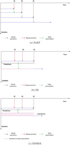
ES is an alternative ensemble-based data assimilation scheme. ES does not assimilate the data sequentially in time, but performs a single estimation assimilating all available measurements (${\mathit{d}}_1-{\mathit{d}}_n$) in the space–time domain. In this scheme, the model prediction is first computed for all ensemble members at all time steps. Then all available measurements are assimilated to find the global parameter update. Finally, the model is re-run with the updated parameters to find the final output of the data assimilation framework (see Figure 1b for the illustration). Both the EnKF and the ES use the same equations for the posterior, but in the case of the ES it is applied once for all measurements, whereas for the EnKF it is applied every time when measurements are available.

Emerick and Reynolds (2012) proposed ESMDA as an improvement of ES. In ESMDA, the same data is assimilated iteratively. To account for the fact that the scheme assimilates the same data multiple times, it uses an inflation factor for the error covariance matrix of measurements. This means that instead of making a single linear, potentially large update, multiple smaller linear updates are performed. These iterations can partly resolve reported problems with non-linearity and generally lead to more accurate reconstruction of the “truth” than ES.

2.2.1. Formulation of the data assimilation schemes

To formulate the data assimilation principles, suppose we have the model prediction $\mathit{y}$ which is obtained by running the perfect forward model with pre-defined input model parameters. To map this model output to the measurement space for comparison with the measurements, we use the so-called measurement operator g, which should be highlighted is an operator and not a vector of measurements, i.e. (6) $\mathit{y}=g(m(\mathit{z})),$(6) in which (7) $\mathit{z}={\left(\begin{array}{c}\mathit{x}\mathit{\theta }\end{array}\right)}^{\mathrm{T}}.$(7) Here $\mathit{y}\in {\mathbb{R}}^{N_m}$ is the model forecast mapped to the measurement locations with $N_m$ is the number of measurements, m is model operator which relate input parameters to output, g is the measurement operator which maps the output to measurement space. Furthermore, in Equation (7(7) $\mathit{z}={\left(\begin{array}{c}\mathit{x}\mathit{\theta }\end{array}\right)}^{\mathrm{T}}.$(7) ), $\mathit{z}\in {\mathbb{R}}^{N_x+N_{\theta }}$ is a control or state vector consisting of the state ($\mathit{x}\in {\mathbb{R}}^{N_x}$) and ($\mathit{\theta }\in {\mathbb{R}}^{N_{\theta }}$) represents the parameters with $N_x$ the number of state points and $N_{\theta }$ the number of model parameters.

For a unique given set of parameters, we consider a single simulation of the model and assume this to be the “truth” ($\mathit{y}$). The synthetic measurements are created from the “truth” and perturbed with randomly selected measurement errors and hence can be represented as (8) $\mathit{d}=\mathit{y}+\mathit{e},$(8) where $\mathit{d}\in {\mathbb{R}}^{N_m}$ is the measurement vector and $\mathit{e}\in {\mathbb{R}}^{N_m}$ is the measurement error vector. Measurement errors are assumed to include instrument errors and representation errors and are normally distributed with zero mean and variance defined by the inaccuracies inherent to the measurement device and the representation error (for a discussion on representation error, see Janjić et al. 2018).

Bayes’ theorem defines the joint probability (f) for $\mathit{z}$ and $\mathit{y}$ given the measurements $\mathit{d}$ as (9) $f(\mathit{z},\mathit{y}|\mathit{d})\propto f(\mathit{d}|\mathit{y})f(\mathit{y}|\mathit{z})f(\mathit{z}).$(9) The marginal pdf of $\mathit{z}$ given $\mathit{d}$ can be found as (10) $f(\mathit{z}|\mathit{d})\propto \int f(\mathit{d}|\mathit{y})f(\mathit{y}|\mathit{z})f(\mathit{z})d\mathit{y}=f(\mathit{d}|g(\mathit{z}))f(\mathit{z}).$(10) Assuming the priors to be Gaussian distributed, Equation 10(10) $f(\mathit{z}|\mathit{d})\propto \int f(\mathit{d}|\mathit{y})f(\mathit{y}|\mathit{z})f(\mathit{z})d\mathit{y}=f(\mathit{d}|g(\mathit{z}))f(\mathit{z}).$(10) can be written as (11) $f(\mathit{z}|\mathit{d})\propto \exp \{-\frac{1}{2}J\},$(11) where the cost function J is defined as follows: (12) $J(\mathit{z})=(\mathit{z}-{\mathit{z}}^{\mathrm{f}}{)}^{\mathrm{T}}{\mathbf{C}}_{\mathit{z}\mathit{z}}^{-1}(\mathit{z}-{\mathit{z}}^{\mathrm{f}})+(g(\mathit{z})-\mathit{d}{)}^{\mathrm{T}}{\mathbf{C}}_{\mathit{d}\mathit{d}}^{-1}(g(\mathit{z})-\mathit{d}).$(12) In Equation (12(12) $J(\mathit{z})=(\mathit{z}-{\mathit{z}}^{\mathrm{f}}{)}^{\mathrm{T}}{\mathbf{C}}_{\mathit{z}\mathit{z}}^{-1}(\mathit{z}-{\mathit{z}}^{\mathrm{f}})+(g(\mathit{z})-\mathit{d}{)}^{\mathrm{T}}{\mathbf{C}}_{\mathit{d}\mathit{d}}^{-1}(g(\mathit{z})-\mathit{d}).$(12) ), ${\mathit{z}}^{\mathrm{f}}$ is the prior estimate of $\mathit{z}$, ${\mathbf{C}}_{\mathit{z}\mathit{z}}\in {\mathbb{R}}^{(N_x+N_{\mathit{\theta }})\times (N_x+N_{\mathit{\theta }})}$ is the error covariance of ${\mathit{z}}^{\mathrm{f}}$, and ${\mathbf{C}}_{\mathit{d}\mathit{d}}\in {\mathbb{R}}^{N_m\times N_m}$ is the error covariance of measurements. The ensemble consists of simulations with each a different parameter value. This approach is based on the assumption that model state error is mainly caused by uncertain parameters, and that the parameter errors determine the state errors. The Kalman filter formulation can be derived by assuming the linear operator and minimisation of the cost function (Equation 12(12) $J(\mathit{z})=(\mathit{z}-{\mathit{z}}^{\mathrm{f}}{)}^{\mathrm{T}}{\mathbf{C}}_{\mathit{z}\mathit{z}}^{-1}(\mathit{z}-{\mathit{z}}^{\mathrm{f}})+(g(\mathit{z})-\mathit{d}{)}^{\mathrm{T}}{\mathbf{C}}_{\mathit{d}\mathit{d}}^{-1}(g(\mathit{z})-\mathit{d}).$(12) ). For further details, see Evensen, Vossepoel, and van Leeuwen (2022). Below, the main features of the different assimilation schemes are presented, the algorithms are presented in more detail in the Appendix.

EnKF: In the case of EnKF, multiple realisations of the forward model are being performed. The Kalman equation for each of the ensemble member $i\in N_{\mathrm{e}}$ can be written as (13) ${\mathit{z}}_i^{\mathrm{a}}={\mathit{z}}_i^{\mathrm{f}}+{\mathbf{C}}_{\mathit{z}\mathit{z}}^e{\mathbf{G}}^{\mathrm{T}}(\mathbf{G}{\mathbf{C}}_{\mathit{z}\mathit{z}}^e{\mathbf{G}}^{\mathrm{T}}-{\mathbf{C}}_{\mathit{d}\mathit{d}}{)}^{-1}({\mathit{d}}_i-\mathbf{G}({\mathit{z}}_i^{\mathrm{f}})),$(13) where ${\mathit{z}}^{\mathrm{a}}$ represents the analysis estimate and ${\mathit{z}}^{\mathrm{f}}$ represents the prior estimate and ${\mathbf{C}}_{\mathit{z}\mathit{z}}^e$ is termed as the model covariance matrix. Here (14) ${\mathit{d}}_i=\mathit{d}+{\mathit{ϵ}}_i$(14) represents the perturbed measurements for each ith member, with ${\mathit{ϵ}}_i$ having the same distribution as the measurement errors $\mathit{e}$ in Equation (8(8) $\mathit{d}=\mathit{y}+\mathit{e},$(8) ), following the approach of Burgers, van Leeuwen, and Evensen (1998).

In the implementation of the EnKF in this study, the update equation (Equation 13(13) ${\mathit{z}}_i^{\mathrm{a}}={\mathit{z}}_i^{\mathrm{f}}+{\mathbf{C}}_{\mathit{z}\mathit{z}}^e{\mathbf{G}}^{\mathrm{T}}(\mathbf{G}{\mathbf{C}}_{\mathit{z}\mathit{z}}^e{\mathbf{G}}^{\mathrm{T}}-{\mathbf{C}}_{\mathit{d}\mathit{d}}{)}^{-1}({\mathit{d}}_i-\mathbf{G}({\mathit{z}}_i^{\mathrm{f}})),$(13) ) is applied whenever the measurements are available. At each update step, elements of Equation (13(13) ${\mathit{z}}_i^{\mathrm{a}}={\mathit{z}}_i^{\mathrm{f}}+{\mathbf{C}}_{\mathit{z}\mathit{z}}^e{\mathbf{G}}^{\mathrm{T}}(\mathbf{G}{\mathbf{C}}_{\mathit{z}\mathit{z}}^e{\mathbf{G}}^{\mathrm{T}}-{\mathbf{C}}_{\mathit{d}\mathit{d}}{)}^{-1}({\mathit{d}}_i-\mathbf{G}({\mathit{z}}_i^{\mathrm{f}})),$(13) ) consist of the available information at that specific assimilation step in which ${\mathit{z}}_i^{\mathrm{a}},{\mathit{z}}_i^{\mathrm{f}}\in {\mathbb{R}}^{N_x+N_{\theta }}$ represent the analysis and forecast vector, respectively, at that specific data assimilation time for $i\mathrm{th}$ ensemble member, ${\mathbf{C}}_{\mathit{z}\mathit{z}}\in {\mathbb{R}}^{(N_x+N_{\mathit{\theta }})\times (N_x+N_{\mathit{\theta }})}$ is the error covariance of ${\mathit{z}}_i^{\mathrm{f}}$ at that specific data assimilation time and ${\mathbf{C}}_{\mathit{d}\mathit{d}}\in {\mathbb{R}}^{N_m\times N_m}$ is the error covariance of measurements for that specific data assimilation time.

Ensemble smoother (ES): ES equations are essentially the same equations as those of the EnKF. Just like the equations for the EnKF, Equation 13(13) ${\mathit{z}}_i^{\mathrm{a}}={\mathit{z}}_i^{\mathrm{f}}+{\mathbf{C}}_{\mathit{z}\mathit{z}}^e{\mathbf{G}}^{\mathrm{T}}(\mathbf{G}{\mathbf{C}}_{\mathit{z}\mathit{z}}^e{\mathbf{G}}^{\mathrm{T}}-{\mathbf{C}}_{\mathit{d}\mathit{d}}{)}^{-1}({\mathit{d}}_i-\mathbf{G}({\mathit{z}}_i^{\mathrm{f}})),$(13) , they are found by equating the cost function gradient equal to zero to find its minimum and defining the covariances around its mean (Evensen 2018).

In the case of ES, all measurements are assimilated in a single step to find a global update which means the measurement vector(${\mathit{d}}_i$) in Equation (13(13) ${\mathit{z}}_i^{\mathrm{a}}={\mathit{z}}_i^{\mathrm{f}}+{\mathbf{C}}_{\mathit{z}\mathit{z}}^e{\mathbf{G}}^{\mathrm{T}}(\mathbf{G}{\mathbf{C}}_{\mathit{z}\mathit{z}}^e{\mathbf{G}}^{\mathrm{T}}-{\mathbf{C}}_{\mathit{d}\mathit{d}}{)}^{-1}({\mathit{d}}_i-\mathbf{G}({\mathit{z}}_i^{\mathrm{f}})),$(13) ) consists of all information at all data assimilation steps. This implies that ${\mathit{z}}_i^{\mathrm{a}},{\mathit{z}}_i^{\mathrm{f}}\in {\mathbb{R}}^{(N_x+N_{\theta })\ast t}$, the analysis and forecast vectors, consist of the state-parameter vector for all time steps until the end of data assimilation window for a specific, $i^{\mathrm{th}}$, ensemble member, where ${\mathbf{C}}_{\mathit{z}\mathit{z}}\in {\mathbb{R}}^{(N_x+N_{\mathit{\theta }})\ast t\times (N_x+N_{\mathit{\theta }})\ast t}$ is the spatio-temporal error covariance of ${\mathit{z}}_i^{\mathrm{f}}$, and ${\mathbf{C}}_{\mathit{d}\mathit{d}}\in {\mathbb{R}}^{(N_m\times N_m)\ast t}$ is the error covariance of measurements for all data assimilation steps.

ESMDA: ESDMA can also be derived from Bayes theory and has the same theoretical basis as ES. However, rather than computing the analysis in a single iteration, it is obtained in a number of steps, where the posterior ($f(\mathit{z}|\mathit{d})$) is made up of a combination of tempered likelihood functions ($\prod _{j=1}^{N_{\mathrm{m}\mathrm{d}\mathrm{a}}}f(\mathit{d}|g({\mathit{z}}_{j-1}){)}^{\frac{1}{{\alpha }_j}}$) and prior ($f(\mathit{z})$). This implies: (15) $f(\mathit{z}|\mathit{d})=f(\mathit{z})\prod _{j=1}^{N_{\mathrm{m}\mathrm{d}\mathrm{a}}}f(\mathit{d}|g({\mathit{z}}_{j-1}){)}^{\frac{1}{{\alpha }_j}},$(15) where (16) $\sum _{j=1}^{N_{\mathrm{m}\mathrm{d}\mathrm{a}}}\frac{1}{{\alpha }_j}=1.$(16) In these equations, ${\alpha }_j$ is the tempering parameter for the $j\mathrm{th}$ recursive step to inflate the measurement error to damp the model update. With this formulation, the cost function can be written as (17) $J({\mathit{z}}_{i,j+1})=({\mathit{z}}_{i,j+1}-{\mathit{z}}_{i,j}^{\mathrm{f}}{)}^{\mathrm{T}}{\mathbf{C}}_{\mathit{z}\mathit{z}}^{-1}({\mathit{z}}_{i,j+1}-{\mathit{z}}_{i,j}^{\mathrm{f}})+(g({\mathit{z}}_{i,j+1})-{\mathit{d}}_i-\sqrt{{\alpha }_j}ϵ{)}^{\mathrm{T}}{\alpha }_j{\mathbf{C}}_{\mathit{d}\mathit{d}}^{-1}(g({\mathit{z}}_{i,j+1})-{\mathit{d}}_i-\sqrt{{\alpha }_j}ϵ),$(17) where $J({\mathit{z}}_{i,j+1})$ is the cost function for ensemble i and j + 1 recursive update step. The minimisation of cost function corresponds to maximisation of the each recursion, that is: (18) ${\mathit{z}}_{i,j+1}^{\mathrm{a}}={\mathit{z}}_{i,j}^{\mathrm{f}}+{\mathbf{C}}_{\mathit{z}\mathit{z}}^{e,j}{\mathbf{G}}^{\mathrm{T}}(\mathbf{G}{\mathbf{C}}_{\mathit{z}\mathit{z}}^{e,j}{\mathbf{G}}^{\mathrm{T}}-{\alpha }_j{\mathbf{C}}_{\mathit{d}\mathit{d}}{)}^{-1}({\mathit{d}}_i+\sqrt{{\alpha }_j}ϵ-g({\mathit{z}}_{i,j}^{\mathrm{f}})).$(18) In each step, the measurement error matrix is inflated with ${\alpha }_j$ and measurements are perturbed with $\sqrt{{\alpha }_j}ϵ$. The error covariance matrix is updated for each of the recursive update steps with a new value of ${\alpha }_j$. The ${\alpha }_j$ parameters should satisfy the Equation (16(16) $\sum _{j=1}^{N_{\mathrm{m}\mathrm{d}\mathrm{a}}}\frac{1}{{\alpha }_j}=1.$(16) ) condition assimilate the observations in multiple steps, i.e. with multiple smaller corrections, and at the same time to ensure the measurements do not obtain too much weight. As the same data is assimilated in $N_{\mathrm{m}\mathrm{d}\mathrm{a}}$ iterations, a practical difficulty of the implementation of ESMDA is that $N_{\mathrm{m}\mathrm{d}\mathrm{a}}$ and its coefficients need to be selected prior to the data assimilation. Emerick and Reynolds (2013) suggest choosing α values in decreasing order to ensure that the initial updates are smaller.

3. Synthetic example

An idealised 2D slope geometry is considered to test and illustrate the performance of the data assimilation schemes described in Section 2.2. The geometry of the slope with mechanical and hydraulic boundary conditions is shown in Figure 2. The black circles on the crest and slope represent the measurement locations. The slope undergoes gravity and hydraulic loading (variable hydraulic boundary conditions). To setup the initial stress state of the slope system, gravity loading with steady-state groundwater flow calculations are performed by considering the water level at line CE in Figure 2. In this study, Van Genuchten-Mualem (1976) model is used to simulate the behaviour of unsaturated soil with the properties mentioned in Table 1. After the initial stress state, the slope is subjected to the generally-rising fluctuation ($D_w$) of the water level. The fluctuation of ($D_w$) is shown on the top-right of Figure 2. The changes in hydraulic boundaries associated with this water level fluctuation cause vertical and lateral slope deformations and changes in the factor of safety that are computed with the forward model.

Figure 2. Geometry of the slope (dimensions in m) and black circles represent the measurement points. On the top right, water level fluctuation is shown. The model forecast at the red stars are computed to perform the data assimilation.

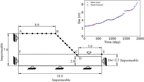
Table 1. “Truth” model parameters for EnKF, ES, ESMDA.

Parameters	Values	Unit
Effective friction angle (${\varphi }^{\prime }$)	25	${}^{\circ }$
Effective cohesion ($c^{\prime }$)	5	kPa
Dilatancy angle (ψ)	0	${}^{\circ }$
$E_{50}^{\mathrm{ref}}$	20,000	kPa
$E_{\mathrm{oed}}^{\mathrm{ref}}$	$E_{50}^{\mathrm{ref}}$	kPa
$E_{\mathrm{ur}}^{\mathrm{ref}}$	2.5$E_{50}^{\mathrm{ref}}$	kPa
Poisson's ratio for unloading/reloading (${\nu }_{\mathrm{ur}}$)	0.2	–
Stress-level dependency (m)	0.5	–
Unsaturated unit weight (${\gamma }_d$)	17	kN/m${}^3$
Saturated unit weight (${\gamma }_s$)	18.5	kN/m${}^3$
Hydraulic conductivity ($k_x=k_y$)	0.12	m/day
VGM parameter ($g_a$)	3.83	$m^{-1}$
VGM parameter ($g_n$)	1.3774	–
VGM parameter ($g_l$)	1.25	–
Saturated volumetric water content (${\theta }_s$)	1.0	–
Residual volumetric water content (${\theta }_r$)	0.062	–

*Note: VGM stands for van Genuchten-Mualem model.

A so-called truth is defined by selecting a unique simulation of the forward model by specifying “true” parameters (Table 1) and the initial state. True model evolution in the form of horizontal displacements at point G (see Figure 2) and the resulting FoS can be seen in Figure 3. The displacements are seen to increase as the water level rises, in conjunction with the effective stress decrease. The FoS is seen to first decrease, most likely due to the reduction in effective stress and the consequential reduction in shear strength due to the friction component, and then increase, most likely due to the reduction in buoyant weight of the material. Both the reduction in shear strength and buoyant weight are due to the increase in the water level, with the details of the geometry and material parameters governing which impact is dominant. The horizontal deformations on the crest-slope are sampled from this forward simulation during a time interval of 150–200 days (with the sample times indicated in the top right sub-figure of Figure 2 by red-stars). Considering the millimetre scale accuracy of measurements devices (such as INSAR, and laser scanners), we have added realistic measurement noise (with zero mean and ${10}^{-7}$ m variance) to the data, and then these synthetic measurements are assimilated into an FEM model with the same initial conditions and water level fluctuations as the truth simulation, but with different parameter distributions for strength and stiffness as shown in Table 2.

Figure 3. Evolution of horizontal displacement (m) at point G on the slope and FoS evolution based on the true model parameters (see in Table 1) and water level fluctuation (see in Figure 2)

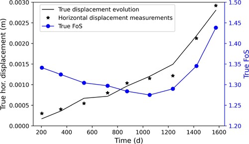
Table 2. Initial estimation of model parameters.

Parameters	Parameter values	Distribution	Unit
Effective friction angle (${\varphi }^{\prime }$)	$\mu =30,\sigma =3$	Normal	${}^{\circ }$
$E_{50}^{\mathrm{ref}}$	$\mu =25000,\sigma =2500$	Normal	kPa

EnKF, ES and ESMDA are tested in this setup to estimate the two most sensitive parameters, the friction angle (${\varphi }^{\prime }$) and secant stiffness at reference pressure ($E_{50}^{\mathrm{ref}}$) parameters, and then finally the FoS estimation. For each of the schemes, the ensemble has 50 members. This ensemble size was demonstrated by Mohsan, Vardon, and Vossepoel (2021) to be sufficient to reliably assimilate the data using a similar case study. This highlights the potential advantage of ensemble type approaches. The performance of the data assimilation schemes is evaluated by comparing their ability to reconstruct the truth within the assumed accuracy of the measurements and by comparing computational performance.

The setup of the experiments is shown in Table 3. In the first experiment, EnKF is implemented as the data assimilation scheme, and the measurements are assimilated sequentially in time. For this setup, estimates of parameter values, displacement and FoS are available at each assimilation step. There are two variants of the test case, with a shorter and longer availability of measurements. For a shorter period (indicated by -s), measurements are assimilated until 1053 days and for a longer period (indicated by -l) measurements are assimilated until 1575 days. In the second test case, two independent experiments are performed with ES: ES-s and ES-l, with the same data availability as for the EnKF test cases. Then, ESMDA is applied in three different cases (named as ESMDA(x2e), ESMDA(x4e) and ESMDA(x4d)) to see the effect of choosing the number of update steps and the effect of α values. For ESMDA(x2e), there are two iterations by taking equal α values, while in ESMDA(x4e), there are four iterations with equal α values. For ESMDA(x4d), the measurements are assimilated in four iterations using decreasing α values. Furthermore, each of these experiments (ESMDA(x2e), ESMDA(x4e) and ESMDA(x4d)) are subdivided into two in the same way as for EnKF and ES with shorter and longer measurement availabilities.

4. Results

The data assimilation performance is evaluated with the estimation of the selected parameters ($E_{50}^{\mathrm{ref}}$ and ${\varphi }^{\prime }$), displacement, FoS estimation and by the computation time. While FoS estimation is the primary target, the parameter and displacement estimation are prerequisites for the FoS to be reliably predicted.

Table 3. Experimental plan for different data assimilation schemes.

Test case name	Data assimilation scheme	α values
EnKF-s, EnKF-l	EnKF	[–]
ES-s, ES-l	ES	[–]
ESMDA(x2e)-s, ESMDA(x2e)-l	ESMDA(x2e)	[2,2]
ESMDA(x4e)-s, ESMDA(x4e)-l	ESMDA(x4e)	[4,4,4,4]
ESMDA(x4d)-s, ESMDA(x4d)-l	ESMDA(x4d)	[9.3,7.0,4.0,2.0]

4.1. Parameter estimation

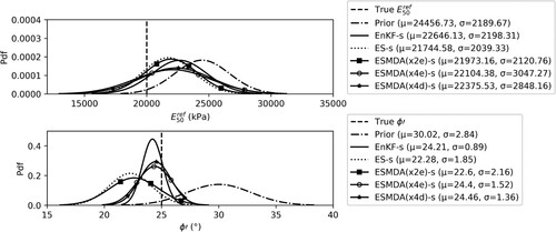
Figure 4 presents the parameter estimation ($E_{50}^{\mathrm{ref}}$ and ${\varphi }^{\prime }$) after assimilating the measurement for the shorter period. The true parameters, prior parameter distribution, and the posterior estimate using EnKF-s, ES-s, ESMDA(x2e)-s, ESMDA(x4e)-s and ESMDA(x4d)-s are presented for both parameters. By construction, the distribution of the true parameters and the prior parameter distribution are the same for all test cases. After the assimilation of measurements, the posterior parameter mean (μ) and standard deviation (σ) are computed from the ensemble, and the resulting normal distributions with these statistical moments are shown in Figure 4. The mean (μ) obtained from the posterior distribution of $E_{50}^{\mathrm{ref}}$ is closer to the true value of $E_{50}^{\mathrm{ref}}$ than the prior mean for all the data assimilation schemes. But in most cases, the width of the posterior distribution of $E_{50}^{\mathrm{ref}}$ has not changed significantly by assimilating the measurements for this (shorter) time period. The limited amount of information from the measurements has thus resulted in a shift of the distribution relative to the prior, but has not narrowed the ensemble spread. In the estimation of ${\varphi }^{\prime }$, a significant change from the prior to the posterior distribution can be seen in all cases. In the cases of EnKF-s, ESMDA(x4e)-s and ESMDA(x4d)-s: the posterior mean moves towards the true value and the standard deviations are smaller than that of the prior distribution. The parameter estimates of the ES-s and ES(x2e)-s move in the direction of the mean, but overshoot significantly the true ${\varphi }^{\prime }$, with the standard deviation only reducing slightly.

Figure 4. Estimation of parameters ($E_{50}^{\mathrm{ref}}$ and ${\varphi }^{\prime }$) by EnKF-s, ES-s, ESMDA(x2e)-s, ESMDA(x4e)-s and ESMDA(x4d)-s.

To study the effect of measurement assimilation for a longer period, Figure 5 presents the parameter estimation results after using the measurements available until 1575 days. The posterior improves substantially for the estimation of $E_{50}^{\mathrm{ref}}$ for all the data assimilation schemes as compared to the results in Figure 4; the mean estimates of $E_{50}^{\mathrm{ref}}$ are closer to the true value and their standard deviation is reduced, although the distribution is still relatively broad. This gives the impression that when data are assimilated over a longer period, a more accurate estimate is achieved. On the other hand, the estimate of ${\varphi }^{\prime }$ changes relatively little compared to the results of the shorter period of assimilation as presented in Figure 4. This also highlights that the estimates of ${\varphi }^{\prime }$ in the earlier assimilation steps are reasonably close to the truth.

4.2. Displacement ensemble estimation

This section presents the displacement evolution based on the true, prior and estimated parameters. The displacement evaluation is studied in the form of horizontal displacement of a point G (see Figure 2) on the slope, which is towards the top of the slope, to capture the largest displacements. Figures 6 and 7 illustrate the displacements computed using estimated parameters by assimilating the measurements for shorter and longer periods, respectively. The black line represents the true model evolution based on true model parameters, and the synthetic measurements are represented by black stars. The prior horizontal displacement ensemble (in green) is computed using the prior parameter distribution and as a direct result of initially poorly selected parameter values, it has lower horizontal displacements than the truth. It should be noted that with another initial selection this could be different. Detailed results in the form of the ensemble mean and spread only from EnKF and ES are presented to keep the figures readable – and these represent the best and worst performing methods in Section 4.1. For the other experiments (ESMDA(x2e), ESMDA(x4e) and ESMDA(x4d)), only the mean of the displacement ensemble is plotted.

Figure 5. Estimation of parameters ($E_{50}^{\mathrm{ref}}$ and ${\varphi }^{\prime }$) by EnKF-l, ES-l, ESMDA(x2e)-l, ESMDA(x4e)-l and ESMDA(x4d)-l.

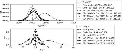
Figure 6. Data assimilation estimate of the horizontal displacement at point G on the slope based on true, prior and estimated parameters with EnKF-s, ES-s, ESMDA(x2e)-s, ESMDA(x4e)-s and ESMDA(x4d)-s. The EnKF-s, ESMDA(x4e)-s and ESMDA(x4d)-s means are overlapping. Furthermore, the mean of ES-s and ESMDA(x2e)-s are also overlapping.

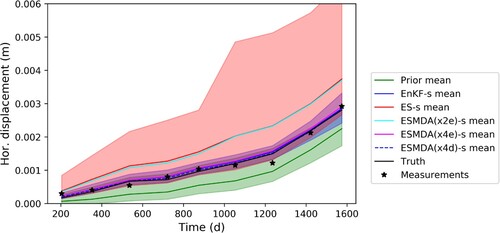
Figure 7. Data assimilation estimate of the horizontal displacement at point G on the slope based on true, prior and estimated parameters with EnKF-l, ES-l, ESMDA(x2e)-l, ESMDA(x4e)-l and ESMDA(x4d)-l. The EnKF-l, ESMDA(x4e)-l and ESMDA(x4d)-l means are overlapping. Furthermore, the mean of ES-l and ESMDA(x2e)-l are also overlapping.

It can be seen from Figure 6 that the mean obtained with EnKF-s, ESMDA(x4e)-s and ESMDA(x4d)-s experiments are very close to the true value. This is because a significant update of the parameters (especially ${\varphi }^{\prime }$) is obtained by assimilating the measurements for a shorter period. In the case of ES-s (and ES(x2e)-s), ${\varphi }^{\prime }$ overshoots the true value and the posterior of the ES-s (and ESMDA(x2e)-s) estimation has a wider spread than that of the EnKF-s estimation (see Figure 4). The posterior distributions of $E_{50}^{\mathrm{ref}}$ are similar for all the assimilation methods and cannot be the main cause of the differences. Due to the difference in ${\varphi }^{\prime }$ estimation, the displacement ensembles produced by the ES-s (and ESMDA(x2e)-s) estimated parameters have a wider spread and compare not as favourably to the true displacement as the other posterior distributions. Furthermore, ES-s and ESMDA(x2e)-s show a larger displacement magnitude than the truth and EnKF-s because they underestimate the strength (${\varphi }^{\prime }$) as compared to the EnKF-s estimation.

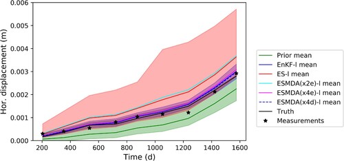
Figure 7 presents the displacement ensemble with estimated parameters after assimilating measurements for a longer period. It can be seen that there is a limited improvement in the distributions. For example, the ES-l (ESMDA(x2e)-l) case the posterior ensemble spread of the displacements is slightly reduced as compared to its posterior as illustrated in Figure 6. In addition, the ensemble means of ES-l and ESMDA(x2e)-l move slightly towards the true model evolution. This improvement is not easily observed for the EnKF-l, ESMDA(x4e)-l and ESMDA(x4d)-l ensemble predictions of deformation, which have already experienced relatively large updates in the first few assimilation steps.

This limited improvement in the simulation of the displacements is caused by a notable improvement of $E_{50}^{\mathrm{ref}}$ and a more limited improvement in ${\varphi }^{\prime }$. It is concluded that in the earlier part of the analysis different combinations of parameters may result in similar displacements. However, as the time increases, so does the loading (the water level), which results in further constraints to the analysis enabling the data assimilation to better identify the two values of the parameters.

4.3. Factor of safety estimation

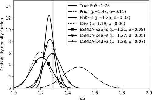
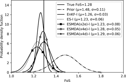
Obtaining an accurate estimate of the FoS is the ultimate goal of this study. As the true distribution of the FoS is not defined, a narrow distribution, i.e. a precise estimate, of the FoS is not necessarily the best result. The FoS estimation is computed by using true parameters, prior parameters and estimated posterior parameters by EnKF, ES, ESMDA, ESMDA(x2e), ESMDA (x4e) and ESMDA(x4d). Again, the estimated parameters from shorter and longer assimilation periods are used, with the FoS evaluated in both cases at the end time, after 1575 days.

Figure 8 shows the FoS at the end of the simulation time, based on the estimated parameters obtained by assimilating the measurement for the shorter period. It can be seen from Figure 8 that the FoS with prior parameters results in a distribution with mean (${\mu }_{\mathrm{fos}}=1.48$) and standard deviation (${\sigma }_{\mathrm{fos}}=0.11$). The true FoS falls within this distribution, yet is significantly lower than the mean FoS calculated using the prior distribution. The true FoS and prior FoS are computed with true and prior parameters by using the strength reduction method. The FoS estimation is considered to be best if it is close to true FoS (accurate). The FoS obtained with EnKF-s is both more accurate and has a smaller standard deviation than ESMDA(x4e)-s, ESMDA(x4d)-s, ESMDA(x2e)-s and ES-s. ES-s and ESMDA(x2e)-s give approximations that are less accurate than the other methodologies. This FoS estimation can be explained by the estimation of parameters, especially ${\varphi }^{\prime }$, as the FoS is calculated by the strength reduction method in which ${\varphi }^{\prime }$ has a significant contribution.

Figure 8. Probability distribution of the FoS at the end time (after 1575 days) based on true parameters, prior parameters and estimated parameters with EnKF-s, ES-s, ESMDA(x2e)-s, ESMDA(x4e)-s and ESMDA(x4d)-s.

Figure 9 illustrates FoS at the end of the simulation time, based on the estimated parameters obtained by assimilating the measurement for the longer period. The result is very similar to the one presented in Figure 8. This is because the FoS depends mostly on the shear strength parameters and has only a slight dependence on stiffness parameters. There is not a significant improvement in the estimation of ${\varphi }^{\prime }$ by assimilating measurements after a shorter period.

Figure 9. Probability distribution of the FoS at the end time (after 1575 days) based on true parameters, prior parameters and estimated parameters with EnKF-l, ES-l, ESMDA(x2e)-l, ESMDA(x4e)-l and ESMDA(x4d)-l

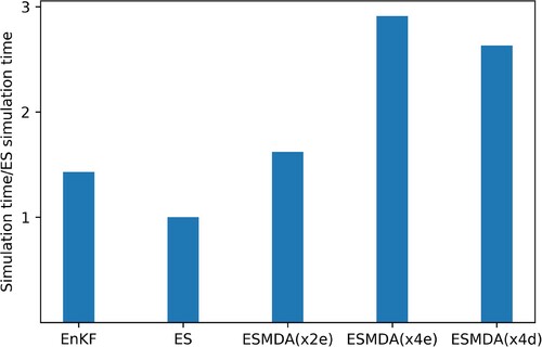
4.4. Computation time

For a practical application of the workflow presented in this study, the computation time of the data assimilation is important, i.e. the computation time of both the forward analyses and the data assimilation steps. Therefore, we divide the framework into two parts, i.e. (i) forward model runs and (ii) data assimilation steps. In this research, the forward model (FEM analysis) is more computationally expensive than the data assimilation part. EnKF is a sequential data assimilation method in which measurements are assimilated whenever they are available and the forward model is re-run with the resulting estimated parameters. In ES, the forward model is run only two times: once with prior parameters and once more with estimated parameters. In ESMDA, the forward model is run for $N_{\mathrm{mda}}$ times during the assimilation and lastly with the estimated parameters. Table 4 shows that the EnKF needs more forward runs ($N_{\mathrm{da}}+1=10$) than ESMDA(x4) ($N_{\mathrm{mda}}+1=5$) and ES (=2). The forward runs in EnKF have variable simulation times (they run until the next measurement is available), but this has a limited impact as the initial solution of the equations takes the majority of the simulation time. On top of that, the number of data assimilation steps is also higher for the EnKF, followed by ESMDA(x4) and ES. Based on this, the EnKF is theoretically the most computationally expensive followed by ESMDA(x4d and e) and then ES.

Table 4. Breakdown of computation time for different schemes for one ensemble member ($N_{\mathrm{da}}$= data assimilation steps, $N_{\mathrm{mda}}$=multiple data assimilation ).

Methodology	Forward model runs	Data assimilation steps
EnKF	$N_{\mathrm{da}}+1$	$N_{\mathrm{da}}$
ES	2	1
ESMDA	$N_{\mathrm{mda}}+1$	$N_{\mathrm{mda}}$

A complicating factor is that the FEM software used in this study delivers output at intermediate steps but is not able to do so at predefined data assimilation steps, without restarting a calculation, i.e. resolving a linear system of equations. Therefore, the smoothers are more computationally expensive in practice that in theory. In Figure 10, the total simulation time for each of the methods considered, normalised to the ES simulation time. The results show that in our implementation EnKF is 1.43 times more computationally expensive than ES. The other methods take ≈ 1.6 times (ESMDA(x2e)), ≈ 2.9 times (ESMDA(x4e)) and ≈ 2.6 times (ESMDA(x4d)) more simulation time than ES.

Figure 10. Computation performance for different data assimilation methods in the present setup of data assimilation.

5. Discussion

There are four important points that can be discussed based on this study and its future directions. First, the data assimilation methods (especially EnKF, ESMDA(x4e) and ESMDA(x4d)) give promising results for reliable parameter estimation, displacement estimation and FoS estimation. it is shown that with limited ensemble sizes, data assimilation can be carried out with detailed numerical simulations, allowing full physics to be captured. The EnKF provides better estimates of parameters, state and FoS than the other schemes. This can be due to the reason that the EnKF deals relatively well with weakly non-linear models and/or its recursive nature of sequential assimilation. In the EnKF as implemented in this study, we are sequentially updating the parameters at each assimilation step and re-rerun the model with estimated parameters. Sequential parameter estimation in a realistic case, i.e. in a case of an imperfect model where model and observations may not be fully consistent, may however cause inconsistency between the analysis and the observations in the intermediate steps of the model, where the early data may match the prediction less well than at the end of the simulation. In the case where a model is not perfect, for example because it does not include all processes (e.g. creep), this imperfect match would probably not hamper the forecast of the model into the immediate future. Building on this observation, poorly matching initial data may eventually be used to detect and analyse model error. The ES and ESMDA(x2e) are shown to not perform well. This can be due to the reason that the ES is not designed to perform with a non-linear model. The other methods such as ESMDA(x4e) and ESMDA(x4d) give good results, using all of the measurements at the same time. The resulting evolution of deformation can be considered more physically representative and consistent with the slope having the same material (behaviour) throughout. The results suggest that in comparison to ES, the MDA steps in ESMDA provide corrections for the linear approximation of ES when applied to a non-linear model. The ESMDA performance can be enhanced by choosing more iterations (MDA steps) as we have seen in our experiments by comparing ESMDA(x2e) and ESMDA(x4e). It can be seen further that the choice of α values (in ESMDA) does not make a significant difference in our study perhaps due to the nature of the perfect model experiment (synthetic twin). Furthermore, better approximations of parameter, state and FoS can be achieved by assimilating the measurements for a longer period compared to a shorter period.

Second, it is difficult to assimilate the measurements in an imperfect model. By doing so, one may get unrealistic estimates of parameters. Such unrealistic parameter estimates will not be able to provide improved estimations of the state of the system. Therefore, it is advised to consider the important physical processes in the numerical model simulations (or consider the representation errors in the model) so that the numerical model prediction qualitatively matches that of the measurement trend before the assimilation. This may also affect the choice of assimilation method. The smoothers attempt to match the data throughout the simulation time, whereas the EnKF assimilates the data sequentially and therefore allows the simulation -especially when the model is imperfect- to progressively drift away from the measurements at early times as the simulation continues. This implies that to use smoothers there is a higher requirement for the model to well represent all processes, or to explicitly account for model error in the data asimilation formulation. Naturally, a better representation of all processes will lead to a higher confidence in the model forecast, especially at longer terms.

Third, having a forward model software which can calculate solutions at prescribed timesteps and extract results at specified intermediate steps can improve the computation performance of smoothers. It could be further investigated how interpolation would allow the performance to be improved while resulting in effective assimilation.

Fourth, this study is limited to a homogeneous slope. One may test these data assimilation methodologies by considering the spatial variability in the slope domain, frequency of measurements and the period with available measurements.

6. Conclusion

In this study, different data assimilation schemes namely EnKF, ES and ESMDA are implemented to estimate selective constitutive model parameters (i.e. $E_{50}^{\mathrm{ref}}$ and ${\varphi }^{\prime }$) in a slope stability system. These estimated parameters are then used to estimate the state and FoS of the system. The results of a synthetic twin experiment show that EnKF estimates an FoS that is close to the true FoS with a small standard deviation. ESMDA, a smoother with four iterative assimilation steps, also estimates an FoS close to the truth with a distribution that has a higher standard deviation. The ES and ESMDA (with two iterative assimilations) are not able to reconstruct the true FoS very well, most likely due to the mostly linear updates of these schemes. The theoretical computation time required by the ES is the smallest, followed by ESMDA with two iterative assimilation steps, ESMDA with four assimilation steps, and EnKF. Due to some forward model limitations in the commercial software used (i.e. PLAXIS cannot output the results at specific data assimilation steps without additional computations to resolve the system of equations), ESMDA needs relatively more computation time than the EnKF and ES.

Disclosure statement

No potential conflict of interest was reported by the author(s).

Additional information

Funding

This research is funded via the i2MON project of the EU HORIZON 2020 programme, via the Research Fund for Coal and Steel (RFCS) with project number 800689.

Appendix

In this section, the algorithms for the different data assimilation schemes are presented.

Algorithm 1 Ensemble Kalman Filter (EnKF)

Input: ${\mu }_{\mathrm{phi}}^{\mathrm{o}},{\sigma }_{\mathrm{phi}}^{\mathrm{o}},{\mu }_e^{\mathrm{o}},{\sigma }_e^{\mathrm{o}},{\sigma }_{\mathrm{obs}}^2,\mathrm{Dw},c,{\mathbf{D}}_{\mathrm{truth}},G$
Output: ${\mathbf{Z}}^{\mathrm{a}},,\mathbf{F}$
1 Initialisation
2 Read input and define variables
3 Initialise required vector and matrices
4 ${\mathit{e}}^{\mathrm{o}}=\mathcal{N}({\mu }_e^{\mathrm{o}},{\sigma }_e^{\mathrm{o}})$	⊳ prior $E_{50}^{\mathrm{ref}}$ sampling
5 ${\mathit{p}}^{\mathrm{o}}=\mathcal{N}({\mu }_{\mathrm{phi}}^{\mathrm{o}},{\sigma }_{\mathrm{phi}}^{\mathrm{o}})$	⊳ prior ${\varphi }^{\prime }$ sampling
6 while $t\le t_{\mathrm{assim}}$ do
7  Read water level time series $\mathrm{Dw}(t)$
8  while $i\le N_e$ do	⊳ loop over ensembles
9   Instructions to set up realisation i
10   $\mathit{x}=\mathrm{h}\mathrm{m}({\mathit{e}}^{\mathrm{t}}(i),{\mathit{p}}^{\mathrm{t}}(i),\mathrm{Dw},p)$	⊳ HM analysis and extract $\mathit{x}$
11   $f=\mathrm{s}\mathrm{a}(\mathrm{h}\mathrm{m}({\mathit{e}}^{\mathrm{t}}(i),{\mathit{p}}^{\mathrm{t}}(i),\mathrm{Dw},p)$	⊳ FoS analysis
12   $\mathit{f}(i)=f$	⊳ save f in vector $\mathit{f}$
13   ${\mathbf{X}}_t^{\mathrm{f}}[:,i]=\mathit{x}$	⊳ save $\mathit{x}$ in matrix
14  ${\mathbf{Z}}_t^{\mathrm{f}}=({\mathbf{X}}_t^{\mathrm{f}},{\mathit{e}}^{\mathrm{t}},{\mathit{p}}^{\mathrm{t}}$)
15  ${\mathbf{C}}_{\mathit{z}\mathit{z}}^e=\mathrm{cov}({\mathbf{Z}}_t^{\mathrm{f}})$
16  ${\mathit{d}}_t^l={\mathit{d}}_t+{ϵ}_t^l,l=1,2,\dots .N_e$
17  ${\mathbf{Z}}_t^{\mathrm{a}}={\mathbf{Z}}_t^{\mathrm{f}}+{\mathbf{C}}_{\mathit{z}\mathit{z}}^e{\mathbf{G}}^{\mathrm{T}}(\mathbf{G}{\mathbf{C}}_{\mathit{z}\mathit{z}}^e{\mathbf{G}}^{\mathrm{T}}+{\mathbf{C}}_{\mathit{d}\mathit{d}}{)}^{-1}({\mathbf{D}}_t-\mathbf{G}{\mathbf{Z}}_t^{\mathrm{f}})$

Algorithm 2 Ensemble smoother (ES)

Input: ${\mu }_{\mathrm{phi}}^{\mathrm{o}},{\sigma }_{\mathrm{phi}}^{\mathrm{o}},{\mu }_e^{\mathrm{o}},{\sigma }_e^{\mathrm{o}},{\sigma }_{\mathrm{obs}}^2,\mathrm{Dw},c,{\mathbf{D}}_{\mathrm{truth}},G$
Output: ${\tilde{\mathbf{Z}}}^{\mathrm{a}}$
1 Initialisation
2 Read input and define variables
3 Initialise required vector and matrices
4 ${\mathit{e}}^{\mathrm{o}}=\mathcal{N}({\mu }_e^{\mathrm{o}},{\sigma }_e^{\mathrm{o}})$	⊳ prior $E_{50}^{\mathrm{ref}}$ sampling
5 ${\mathit{p}}^{\mathrm{o}}=\mathcal{N}({\mu }_{\mathrm{phi}}^{\mathrm{o}},{\sigma }_{\mathrm{phi}}^{\mathrm{o}})$	⊳ prior ${\varphi }^{\prime }$ sampling
6 ${\mathit{\theta }}^{\mathrm{o}}=({\mathit{e}}^o,{\mathit{p}}^o{)}^{\mathrm{T}}$	⊳ prior parameter matrix
7 while $i\le N_e$ do	⊳ loop over ensembles
8  while $t\le t_{\mathrm{assim}}$ do	⊳ loop over timesteps
9   Read water level time series $\mathrm{Dw}(t)$
10   Setup for initial stress state
11   $\mathit{x}=\mathrm{h}\mathrm{m}({\mathit{e}}^{\mathrm{o}}(i),{\mathit{p}}^{\mathrm{o}}(i),\mathrm{Dw},c)$	⊳ HM analysis and extract $\mathit{x}$
12   $f=\mathrm{s}\mathrm{a}(\mathrm{h}\mathrm{m}({\mathit{e}}^{\mathrm{o}}(i),{\mathit{p}}^{\mathrm{o}}(i),\mathrm{Dw},c))$	⊳ FoS analysis
13   ${\mathbf{A}}_i^{\mathrm{f}}[:,t]=\mathit{x}$	⊳ save $\mathit{x}$ in matrix
14   $\mathit{f}(t)=f$	⊳ save f in vector $\mathit{f}$
15 ${\mathbf{Z}}_t^{\mathrm{f}}=({\mathbf{X}}_t^{\mathrm{f}},{\mathit{\theta }}^{\mathrm{o}}{)}^{\mathrm{T}}$	⊳ develop ${\mathbf{Z}}_t^{\mathrm{f}}$ for all time steps
16 $\tilde{\mathbf{Z}}=({\mathbf{Z}}_1^{\mathrm{f}},{\mathbf{Z}}_2^{\mathrm{f}},\dots \cdots {\mathbf{Z}}_{\mathrm{tassim}}^{\mathrm{f}}{)}^{\mathrm{T}}$	⊳ stacking all forcast-parameter matrices
17 ${\tilde{\mathbf{C}}}_{\mathit{z}\mathit{z}}^e=\mathrm{cov}(\tilde{\mathbf{Z}})$	⊳ estimate the spatial-temporal covariance matrix
18 ${\mathit{d}}_t^l={\mathit{d}}_t+{ϵ}_t^l,l=1,2,\dots .N_e$
19 ${\mathit{D}}_t=({\mathit{d}}_t^1,{\mathit{d}}_t^2,{\mathit{d}}_t^{\mathrm{Ne}})$	⊳ develop ${\mathbf{D}}_t$ for all time steps
20 $\tilde{\mathbf{D}}=({\mathbf{D}}_1,{\mathbf{D}}_2,\dots \cdots {\mathbf{D}}_{\mathrm{tassim}}{)}^{\mathrm{T}}$	⊳ stacking all perturbed observations matrices
21 ${\tilde{\mathbf{C}}}_{\mathit{d}\mathit{d}}={\sigma }_{\mathrm{obs}}^2\mathit{I}$
22 Read $\tilde{\mathbf{G}}$ from file
23 ${\tilde{\mathbf{Z}}}^{\mathrm{a}}=\tilde{\mathbf{Z}}+{\tilde{\mathbf{C}}}_{\mathit{z}\mathit{z}}^e{\tilde{\mathbf{G}}}^{\mathrm{T}}(\tilde{\mathbf{G}}{\tilde{\mathbf{C}}}_{\mathit{z}\mathit{z}}^e{\tilde{\mathbf{G}}}^{\mathrm{T}}+{\tilde{\mathbf{C}}}_{\mathit{d}\mathit{d}}{)}^{-1}(\tilde{\mathbf{D}}-\tilde{\mathbf{G}}\tilde{\mathbf{Z}})$	⊳ extract estimated parameters from ${\tilde{\mathbf{Z}}}^{\mathrm{a}}$

Algorithm 3 Ensemble smoother with multiple data assimilation (ESMDA)

Input: ${\mu }_{\mathrm{phi}}^{\mathrm{o}},{\sigma }_{\mathrm{phi}}^{\mathrm{o}},{\mu }_e^{\mathrm{o}},{\sigma }_e^{\mathrm{o}},{\sigma }_{\mathrm{obs}}^2,\mathrm{Dw},c,{\mathbf{D}}_{\mathrm{truth}},\mathbf{G},\alpha$
Output: ${\tilde{\mathbf{Z}}}^{\mathrm{a}}$
1 Initialisation
2 Read input and define variables
3 Initialise required vector and matrices
4 ${\mathit{e}}^{\mathrm{o}}=\mathcal{N}({\mu }_e^{\mathrm{o}},{\sigma }_e^{\mathrm{o}})$	⊳ prior $E_{50}^{\mathrm{ref}}$ sampling
5 ${\mathit{p}}^{\mathrm{o}}=\mathcal{N}({\mu }_{\mathrm{phi}}^{\mathrm{o}},{\sigma }_{\mathrm{phi}}^{\mathrm{o}})$	⊳ prior ${\varphi }^{\prime }$ sampling
6 ${\mathit{\theta }}^{\mathrm{o}}=({\mathit{e}}^o,{\mathit{p}}^o{)}^{\mathrm{T}}$	⊳ prior parameter matrix
7 Select the α vector
8 while $k\le \mathrm{len}(\alpha ):$ do	⊳ loop over α
9 while $i\le N_e$ do	⊳ loop over ensembles
10  while $t\le t_{\mathrm{assim}}$ do	⊳ loop over timesteps
11   Read water level time series $\mathrm{Dw}(t)$	⊳ loop over timesteps
12   Setup for initial stress state
13   $\mathit{x}=\mathrm{h}\mathrm{m}({\mathit{e}}^{\mathrm{k}}(i),{\mathit{p}}^{\mathrm{k}}(i),\mathrm{Dw},c)$	⊳ HM analysis and extract $\mathit{x}$
14   $f=\mathrm{s}\mathrm{a}(\mathrm{h}\mathrm{m}({\mathit{e}}^{\mathrm{k}}(i),{\mathit{p}}^{\mathrm{k}}(i),\mathrm{Dw},c))$	⊳ FoS analysis
15   ${\mathbf{A}}_i^{\mathrm{f}}[:,t]=\mathit{x}$	⊳ save $\mathit{x}$ in matrix
16   $\mathit{f}(t)=f$	⊳ save f in vector $\mathit{f}$
17 ${\mathbf{Z}}_t^{\mathrm{f}}=({\mathbf{X}}_t^{\mathrm{f}},{\mathit{\theta }}^{\mathrm{k}}{)}^{\mathrm{T}}$	⊳ develop ${\mathbf{Z}}_t^{\mathrm{f}}$ for all time steps
18 $\tilde{\mathbf{Z}}=({\mathbf{Z}}_1^{\mathrm{f}},{\mathbf{Z}}_2^{\mathrm{f}},\dots \cdots {\mathbf{Z}}_{\mathrm{tassim}}^{\mathrm{f}}{)}^{\mathrm{T}}$	⊳ stacking all forcast-parameter matrices
19 ${\tilde{\mathbf{C}}}_{\mathit{z}\mathit{z}}^e=\mathrm{cov}(\tilde{\mathbf{Z}})$	⊳ estimate the spatial-temporal covariance matrix
20 ${\mathit{d}}_t^l={\mathit{d}}_t+\sqrt{\alpha (k)}{ϵ}_t^l,l=1,2,\dots .N_e$
21 ${\mathit{D}}_t=({\mathit{d}}_t^1,{\mathit{d}}_t^2,{\mathit{d}}_t^{\mathrm{Ne}})$	⊳ Develop ${\mathbf{D}}_t$ for all time steps
22 $\tilde{\mathbf{D}}=({\mathbf{D}}_1,{\mathbf{D}}_2,\dots \cdots {\mathbf{D}}_{\mathrm{tassim}}{)}^{\mathrm{T}}$	⊳ stacking all perturbed measurements matrices
23 ${\tilde{\mathbf{C}}}_{\mathit{d}\mathit{d}}={\sigma }_{\mathrm{obs}}^2\mathit{I}$
24 Read $\tilde{\mathbf{G}}$ from file
25 ${\tilde{\mathbf{Z}}}^{\mathrm{a}}=\tilde{\mathbf{Z}}+{\tilde{\mathbf{C}}}_{\mathit{z}\mathit{z}}^e{\tilde{\mathbf{G}}}^{\mathrm{T}}(\tilde{\mathbf{G}}{\tilde{\mathbf{C}}}_{\mathit{z}\mathit{z}}^e{\tilde{\mathbf{G}}}^{\mathrm{T}}+\alpha (k){\tilde{\mathbf{C}}}_{\mathit{d}\mathit{d}}{)}^{-1}(\tilde{\mathbf{D}}-\tilde{\mathbf{G}}\tilde{\mathbf{Z}})$	⊳ extract estimated parameters from ${\tilde{\mathbf{Z}}}^{\mathrm{a}}$

References

- Aanonsen, S. I., A. C. Reynolds, and B. Vall‘es. 2009. “The Ensemble Kalman Filter in Reservoir Engineering – A Review.” SPE Journal 14 (3): 393–412. https://doi.org/10.2118/117274-PA
- Bertino, L., G. Evensen, and H. Wackernagel. 2003. “Sequential Data Assimilation Techniques in Oceanography.” International Statistical Review 71 (2): 223–241. https://doi.org/10.1111/j.1751-5823.2003.tb00194.x
- Burgers, G., P. J. Van Leeuwen, and G. Evensen. 1998. “Analysis Scheme in the Ensemble Kalman Filter.” Monthly Weather Review 126 (6): 1719–1724.
- Chen, Y., and D. Zhang. 2006. “Data Assimilation for Transient Flow in Geologic Formations via Ensemble Kalman Filter.” Advances in Water Resources 29 (8): 1107–1122. https://doi.org/10.1016/j.advwatres.2005.09.007
- Ching, J., and K.-K. Phoon. 2015. “Reducing the Transformation Uncertainty for the Mobilized Undrained Shear Strength of Clays.” Journal of Geotechnical and Geoenvironmental Engineering 141 (2): 04014103. https://doi.org/10.1061/(ASCE)GT.1943-5606.0001236.
- Contreras, L.-F., and E. T. Brown. 2019. “Slope Reliability and Back Analysis of Failure with Geotechnical Parameters Estimated Using Bayesian Inference.” Journal of Rock Mechanics and Geotechnical Engineering 11 (3): 628–643. https://doi.org/10.1016/j.jrmge.2018.11.008.
- Emerick, A. A. 2016. “Analysis of the Performance of Ensemble-based Assimilation of Production and Seismic Data.” Journal of Petroleum Science and Engineering 139:219–239. https://doi.org/10.1016/j.petrol.2016.01.029.
- Emerick, A. A., and A. C. Reynolds. 2012. “History Matching Time-lapse Seismic Data Using the Ensemble Kalman Filter with Multiple Data Assimilations.” Computational Geosciences 16 (3): 639–659. https://doi.org/10.1007/s10596-012-9275-5.
- Emerick, A. A., and A. C. Reynolds. 2013. “Ensemble Smoother with Multiple Data Assimilation.” Computers & Geosciences 55:3–15. https://doi.org/10.1016/j.cageo.2012.03.011.
- Evensen, G. 1994. “Sequential Data Assimilation with a Nonlinear Quasi-geostrophic Model Using Monte Carlo Methods to Forecast Error Statistics.” Journal of Geophysical Research: Oceans 99 (C5): 10143–10162. https://doi.org/10.1029/94JC00572.
- Evensen, G. 2009. Data Assimilation: the Ensemble Kalman Filter. Berlin: Springer Science & Business Media.
- Evensen, G. 2018. “Analysis of Iterative Ensemble Smoothers for Solving Inverse Problems.” Computational Geosciences 22 (3): 885–908. https://doi.org/10.1007/s10596-018-9731-y.
- Evensen, G., J. Amezcua, M. Bocquet, A. Carrassi, A. Farchi, A. Fowler, P. L. Houtekamer, C. K. Jones, R. J. de Moraes, M. Pulido, and C. Sampson. 2021. “An International Initiative of Predicting the SARS-COV-2 Pandemic Using Ensemble Data Assimilation.” Foundations of Data Science 3 (3): 413–477. https://doi.org/10.3934/fods.2021001
- Evensen, G., and K. S. Eikrem. 2018. “Conditioning Reservoir Models on Rate Data Using Ensemble Smoothers.” Computational Geosciences 22 (5): 1251–1270. https://doi.org/10.1007/s10596-018-9750-8
- Evensen, G., F. C. Vossepoel, and P. J. van Leeuwen. 2022. Data Assimilation Fundamentals: A Unified Formulation of the State and Parameter Estimation Problem. Cham: Springer Nature.
- Glegola, M. A., P. Ditmar, R. G. Hanea, F. C. Vossepoel, R. Arts, and R. Klees. 2012. “Gravimetric Monitoring of Water Influx into a Gas Reservoir: A Numerical Study Based on the Ensemble Kalman Filter.” SPE Journal 17 (1): 163–176. https://doi.org/10.2118/149578-PA
- Grönlund, T., and H. Stille. 2009. “Probabilistic Approach to Assessing and Monitoring Settlements Caused by Tunneling.” Journal of Geotechnical and Geoenvironmental Engineering 135 (9): 1301–1311.
- Houtekamer, P. L., and H. L. Mitchell. 2005. “Ensemble Kalman Filtering.” Quarterly Journal of the Royal Meteorological Society: A Journal of the Atmospheric Sciences, Applied Meteorology and Physical Oceanography 131 (613): 3269–3289. https://doi.org/10.1256/qj.05.135
- Huang, J., R. Kelly, L. Li, M. Cassidy, and S. Sloan. 2014. “Use of Bayesian Statistics with the Observational Method.” Australian Geomechanics 49 (4): 191–198.
- Janjić, T., N. Bormann, M. Bocquet, J. Carton, S. Cohn, S. L. Dance, S. Losa, et al. 2018. “On the Representation Error in Data Assimilation.” Quarterly Journal of the Royal Meteorological Society 144 (713): 1257–1278. https://doi.org/10.1002/qj.2018.144.issue-713.
- Jiang, S.-H., L. Wang, S. Ouyang, J. Huang, and Y. Liu. 2022. “A Comparative Study of Bayesian Inverse Analyses of Spatially Varying Soil Parameters for Slope Reliability Updating.” Georisk: Assessment and Management of Risk for Engineered Systems and Geohazards 16 (4): 746–765. https://doi.org/10.1080/17499518.2021.1952613
- Juang, C. H., and J. Zhang. 2017. ““Bayesian Methods for Geotechnical Applications” a Practical Guide.” In Geotechnical Safety and Reliability, 215–246. ASCE. https://doi.org/10.1061/9780784480700
- Kalman, R. E. 1960. “A New Approach to Linear Filtering and Prediction Problems.” Journal of Basic Engineering 82 (1): 35–45. https://doi.org/10.1115/1.3662552.
- Kelly, R., and J. Huang. 2015. “Bayesian Updating for One-dimensional Consolidation Measurements.” Canadian Geotechnical Journal 52 (9): 1318–1330. https://doi.org/10.1139/cgj-2014-0338.
- Keppenne, C. L., and M. M. Rienecker. 2003. “Assimilation of temperature into an isopycnal ocean general circulation model using a parallel ensemble Kalman filter.” Journal of Marine Systems 40:363–380. https://doi.org/10.1016/S0924-7963(03)00025-3
- Liu, K., P. J. Vardon, and M. A. Hicks. 2018. “Sequential Reduction of Slope Stability Uncertainty Based on Temporal Hydraulic Measurements Via the Ensemble Kalman Filter.” Computers and Geotechnics95:147–161. https://doi.org/10.1016/j.compgeo.2017.09.019.
- Maucec, M., F. M. De Matos Ravanelli, S. Lyngra, S. J. Zhang, A. A. Alramadhan, O. A. Abdelhamid, and S. A. Al-Garni. 2016. “Ensemble-Based Assisted History Matching with Rigorous Uncertainty Quantification Applied to a Naturally Fractured Carbonate Reservoir.” SPE Annual Technical Conference and Exhibition. https://doi.org/10.2118/181325-MS
- Mavritsakis, A. 2017. “Evaluation of Inverse Analysis methods with Numerical Simulation of Slope Excavation.” MSc thesis, Delft University of Technology, Netherlands.
- Mohsan, M., P. J. Vardon, and F. C. Vossepoel. 2021. “On the Use of Different Constitutive Models in Data Assimilation for Slope Stability.” Computers and Geotechnics 138:104332. https://doi.org/10.1016/j.compgeo.2021.104332.
- Mohsan, M., P. J. Vardon, and F. C. Vossepoel. 2023. “Options for the Implementations of Data Assimilation for Geotechnics.” International Conference of the International Association for Computer Methods and Advances in Geomechanics, 255–262.
- Nævdal, G., T. Mannseth, and E. H. Vefring. 2002. “Near-Well Reservoir Monitoring through Ensemble Kalman Filter.” SPE/DOE Improved Oil Recovery Symposium, (SPE 75235). https://doi.org/10.2118/75235-MS
- Oliver, D. S., and Y. Chen. 2011. “Recent Progress on Reservoir History Matching: A Review.” Computational Geosciences 15 (1): 185–221. https://doi.org/10.1007/s10596-010-9194-2
- Phoon, K.-K., and F. H. Kulhawy. 1999a. “Characterization of Geotechnical Variability.” Canadian Geotechnical Journal 36 (4): 612–624. https://doi.org/10.1139/t99-038.
- Phoon, K.-K., and F. H. Kulhawy. 1999b. “Evaluation of Geotechnical Property Variability.” Canadian Geotechnical Journal 36 (4): 625–639. https://doi.org/10.1139/t99-039.
- Plaxis, B. V.. 2015. Plaxis material models manual. The Netherlands.
- Reichle, R. H., D. B. McLaughlin, and D. Entekhabi. 2002. “Hydrologic Data Assimilation with the Ensemble Kalman Filter.” Monthly Weather Review 130 (1): 103–114.
- Schanz, T., P. Vermeer, and P. G. Bonnier. 2019. “The Hardening Soil Model: Formulation and Verification.” In Beyond 2000 in Computational Geotechnics, 281–296. Routledge.
- Skjervheim, J.-A., and G. Evensen. 2011. “An Ensemble Smoother for Assisted History Matching.” In SPE Reservoir Simulation Symposium, number SPE-141929-MS. Society of Petroleum Engineers.
- Szunyogh, I., E. J. Kostelich, G. Gyarmati, D. Patil, B. R. Hunt, E. Kalnay, E. Ott, and J. A. Yorke. 2005. “Assessing a Local Ensemble Kalman Filter: Perfect Model Experiments with the National Centers for Environmental Prediction Global Model.” Tellus A: Dynamic Meteorology and Oceanography 57 (4): 528–545.
- Van der Krogt, M., T. Schweckendiek, and M. Kok. 2019. “Uncertainty in Spatial Average Undrained Shear Strength with a Site-specific Transformation Model.” Georisk: Assessment and Management of Risk for Engineered Systems and Geohazards 13 (3): 226–236.
- Van Genuchten-Mualem, Y.1976. “A New Model for Predicting the Hydraulic Conductivity of Unsaturated Porous Media.” Water Resources Research 12 (3): 513–522. https://doi.org/10.1029/WR012i003p00513.
- Van Leeuwen, P. J. 1999. “The Time-mean Circulation in the Agulhas region Determined with the Ensemble Smoother.” Journal of Geophysical Research: Oceans 104 (C1): 1393–1404. https://doi.org/10.1029/1998JC900012
- Van Leeuwen, P. J., and G. Evensen. 1996. “Data Assimilation and Inverse Methods in Terms of a Probabilistic Formulation.” Monthly Weather Review 124 (12): 2898–2913. https://doi.org/10.1175/1520-0493(1996)124%3C2898:DAAIMI%3E2.0.CO;2
- Vardon, P. J., K. Liu, and M. A. Hicks. 2016. “Reduction of Slope Stability Uncertainty Based on Hydraulic Measurement Via Inverse Analysis.” Georisk: Assessment and Management of Risk for Engineered Systems and Geohazards 10 (3): 223–240. https://doi.org/10.1080/17499518.2016.1180400
- Wang, C., C. A. Osorio-Murillo, H. Zhu, and Y. Rubin. 2017. “Bayesian Approach for Calibrating Transformation Model From Spatially Varied Cpt Data to Regular Geotechnical Parameter.” Computers and Geotechnics 85:262–273. https://doi.org/10.1016/j.compgeo.2017.01.002.
- Wang, X., X.-S. Wang, N. Li, and L. Wan. 2021. “Bayesian Inversion of Soil Hydraulic Properties From Simplified Evaporation Experiments: Use of Dream(zs) Algorithm.” Water 13 (19): 2614. https://doi.org/10.3390/w13192614.
- Yang, H.-Q., L. Zhang, Q. Pan, K.-K. Phoon, and Z. Shen. 2021. “Bayesian Estimation of Spatially Varying Soil Parameters with Spatiotemporal Monitoring Data.” Acta Geotechnica 16 (1): 263–278. https://doi.org/10.1007/s11440-020-00991-z.
- Zhang, L., Z. Zuo, G. Ye, D. Jeng, and J. Wang. 2013. “Probabilistic Parameter Estimation and Predictive Uncertainty Based on Field Measurements for Unsaturated Soil Slope.” Computers and Geotechnics48:72–81. https://doi.org/10.1016/j.compgeo.2012.09.011.