Physics-Informed neural network solver for numerical analysis in geoengineering

ABSTRACT

Engineering-scale problems generally can be described by partial differential equations (PDEs) or ordinary differential equations (ODEs). Analytical, semi-analytical and numerical analysis are commonly used for deriving the solutions of such PDEs/ODEs. Recently, a novel physics-informed neural network (PINN) solver has emerged as a promising alternative to solve PDEs/ODEs. PINN resembles a mesh-free method which leverages the strong non-linear ability of the deep learning algorithms (e.g. neural networks) to automatically search for the correct spatial-temporal responses constrained by embedded PDEs/ODEs. This study comprehensively reviews the current state of PINN including its principles for the forward and inverse problems, baseline algorithms for PINN, enhanced PINN variants combined with special sampling strategies and loss functions. PINN shows an easier modelling process and superior feasibility for inverse problems compared to conventional numerical methods. Meanwhile, the limitations and challenges of applications of current PINN solvers to constitutive modelling and multi-scale/phase problems are also discussed in terms of convergence ability and computational costs. PINN has exhibited its huge potential in geoengineering and brings a revolutionary way for numerous domain problems.

KEYWORDS:

• Neural networks
• physics-informed
• machine learning
• soils
• constitutive modelling
• partial differential equations

1. Introduction

In engineering practice, the spatial-temporal responses of systems are often characterized by mathematical formulations such as partial differential equations (PDEs) or ordinary differential equations (ODEs). In the geotechnical domain, PDEs have also been extensively used to model a series of canonical problems such as consolidation (Terzaghi 1925), cavity expansion (Yu 2000) and landslides (Vardoulakis 2002).

To solve PDEs/ODEs, the use of analytical and semi-analytical methods has been fully investigated by many researchers (Zhou et al. 2018; Feng, Ni, and Mei 2019; Ho and Fatahi 2016). Although analytical and semi-analytical solutions are accurate and convenient, they are limited to simple cases such as low-dimensional problems and simple constitutive relations (Zhang, Yin, and Sheil 2023b; Asaoka 1978). Therefore, much attention has been given to numerical techniques to solve PDEs/ODEs, including finite element methods (FEM) (Feyel 2003; Zhu, Yin, and Graham 2001; Earij et al. 2017; Cividini and Gioda 2004), finite difference methods (Zhou, Deng, and Wang 2013; Ma et al. 2020) and meshless numerical methods such as the smoothed particle hydrodynamics (Monaghan 1992) and the material point method (MPM) (Yerro, Rohe, and Soga 2017; Sulsky, Chen, and Schreyer 1994). However, mesh-based numerical methods still dominate the numerical simulation for engineering practice considering the limitations of mesh-free methods. For instance, the stability of MPM is associated with the time integration procedure of dynamic equations, thus the time increment should be significantly small compared with the FEM (Więckowski 2004).

Despite the great success that numerical methods have achieved, their further progress has been restricted by many challenges and limitations, which can be generally summarised in two aspects: (1) the computational costs of numerical methods are high, especially in multiscale and high-dimensional engineering problems, which hinder high-resolution simulations in engineering practice (Geers et al. 2017; Liu et al. 2021); (2) while inverse problems are quite common in the engineering domain, solving inverse problems is prohibitively expensive where abundant computational trials are required to be carefully implemented.

Recently, due to the fast progress of data science and machine learning (ML), physics-informed neural networks (PINNs) have gained a new round of attention and their history can be dated back to the end of the last century (Lee and Kang 1990). Psichogios and Ungar (1992) proposed a hybrid learning method that incorporated physics laws, e.g. mass balance or energy balance, into the network structure, and the results demonstrated that this hybrid physics-informed method can achieve better generalization and extrapolation ability compared to standard “black-box” ML. Lagaris, Likas, and Fotiadis (1998) successfully solved different PDEs/ODEs considering initial/boundary conditions. In this work, the structure of the trial solution was designed to satisfy hard initial/boundary conditions and the other half of the trial solution was obtained from the output of neural networks to satisfy PDEs/ODEs. More recently, Raissi, Perdikaris, and Karniadakis (2019) applied PINNs to directly solve PDEs, in which the loss values on the initial/boundary conditions and the residuals on the PDEs are added to the loss function of neural works. The core of PINNs is incorporating prior information such as known physics laws and PDEs/ODEs into the neural networks. In this way, the outputs generated by the network can be constrained by physics laws. Compared with traditional data-driven approaches, PINNs can successfully alleviate overfitting issues and can still maintain robustness with a small amount of data or even with imperfect data (Zhang, Liu, and Sun 2020). Its potential on both forward and inverse problems has been successfully proved, while PINNs have achieved competitive performance compared with exact values. To date, this novel approach has been extensively used in numerous engineering and scientific problems, such as fluid mechanics (Cai et al. 2022; Sun et al. 2020; Mao, Jagtap, and Karniadakis 2020; Jin et al. 2021), heat transfer (Cai et al. 2021; Cai et al. 2020), solid mechanics (Abueidda et al. 2022; Diao et al. 2023) and material science (Liu and Wang 2019).

The objective of this review is to provide a comprehensive analysis and discussion of the characterizations of current PINNs. First, the basic modelling framework of a PINN-based PDE solver is introduced. Then, different baseline neural networks, variants, sampling methods and loss functions used in PINNs are introduced. Finally, we demonstrate the limitations and challenges of applying PINNs for engineering problems.

2. Framework of PINNs

A general PDE subjected to initial/boundary conditions in engineering problems can be described by (Rao, Sun, and Liu 2021): (1) $\begin{array}{rl}& u_t(t,\mathit{x})+\mathcal{D}[u(t,\mathit{x})]=0,\mathit{x}\in \mathrm{\Omega },t\in [0,T]\\ & u(t,\mathit{x})={\mathcal{B}}_D(t),x\in \mathrm{\partial }{\mathrm{\Omega }}_D,t\in [0,T]\end{array}$(1) (2) $\mathbf{n}\cdot \mathrm{\nabla }u(t,\mathit{x})={\mathcal{B}}_N(t),\mathit{x}\in \mathrm{\partial }{\mathrm{\Omega }}_N,t\in [0,T]$(2) (3) $\begin{array}{rl}& u(0,\mathit{x})={\mathcal{I}}_0(\mathit{x}),\mathit{x}\in \mathrm{\Omega }\\ & u_t(0,\mathit{x})={\mathcal{I}}_1(\mathit{x}),\mathit{x}\in \mathrm{\Omega }\end{array}$(3) where t and x are the temporal and spatial coordinates, u_t(t, x) is the differential of u(t, x) to t, u(t, x) is the hidden solution, $\mathcal{D}$[·] is a nonlinear differentiation operator, $\mathrm{\Omega }$ is the space of input variables, $\mathrm{\partial }{\mathrm{\Omega }}_D$ and $\mathrm{\partial }{\mathrm{\Omega }}_N$ are the Dirichlet and Neumann boundaries, respectively, ${\mathcal{B}}_D(t)$ and ${\mathcal{B}}_N(t)$ are the prescribed functions in Dirichlet and Neumann boundaries, respectively, T is the maximum computation time, n denotes the unit outer normal vector of boundaries, $\mathrm{\nabla }$ is the gradient operator, ${\mathcal{I}}_0(x)$ and ${\mathcal{I}}_1(x)$ 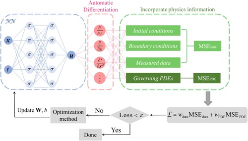are the initial states of the system. A detailed illustration of training PINNs to solve Equation (1) is shown in Figure 1, where x and t are the inputs of the network and u is the output. During the training process, the PINN iteratively adjusts the weights W and biases b of the network, until the loss value is smaller than the tolerance value $\epsilon$. This process is achieved by solving the following optimization problem: (4) ${\theta }^{\ast }=\arg \underset{\theta }{min}\mathcal{L}(\theta t,\mathit{x})$(4) where $\theta$ = [W, b], which are the hyperparameters of the network, $\mathcal{L}$ is the loss function that needs to be minimized.

Figure 1. Framework of a generic PINN (Karniadakis et al. 2021).

In the majority of existing research on PINNs, the weights and biases are fine-tuned predominantly via gradient-based optimization methods. These methods minimize the discrepancy between the predicted and expected outputs by iteratively adjusting the parameters in the direction of the steepest descent of the gradient, which can be generally described by using the following equations (Ruder 2016): (5) ${\theta }^{(n+1)}={\theta }^{(n)}\text{–}\eta \cdot {\mathrm{\nabla }}_{\theta }\mathcal{L}({\theta }^{(n)}t,\mathit{x})$(5) where ${\theta }^{(n)}$ denotes the hyperparameters in the n^th iteration step, $\eta$ is the learning rate. However, a growing body of evidence has demonstrated that gradient descent exhibits pathological behaviour when training PINNs to solve complex PDEs (Wang, Yu, and Perdikaris 2022). Limited research in the field of PINNs has explored the feasibility of employing non-gradient-based optimization methods, such as using a particle swarm optimization approach, rather than gradient descent, to train PINNs (Davi and Braga-Neto 2022). Once the model is well trained, the solution of the embedded PDEs can be solved.

In most literature, the loss function is defined as the mean square error (MSE) of the predictions for the sake of its differentiability (Daolun et al. 2021; Shen et al. 2022; Lu and Mei 2022; Bishop and Nasrabadi 2006), which allows to efficiently implement error backpropagation and gradient descent (Goodfellow, Bengio, and Courville 2016).

The loss function of PINNs generally includes the residual value of governing PDEs/ODEs, initial/boundary conditions and measured data (if available), which has been shown using the following equations: (6) $\mathcal{L}=w_1{\mathcal{L}}_{\mathrm{PDE}}+w_2{\mathcal{L}}_{\mathrm{BC}}+w_3{\mathcal{L}}_{\mathrm{IC}}+w_4{\mathcal{L}}_{\mathrm{data}}$(6) (7) ${\mathcal{L}}_{\mathrm{PDE}}=\Vert u_t(t,\mathit{x})+\mathcal{D}[u(t,\mathit{x})]{\Vert }_{\mathrm{\Omega }\times [0,T]}^2$(7) (8) $\begin{array}{rl}{\mathcal{L}}_{\mathrm{BC}}=& \Vert {u(t,\mathit{x})\text{–}{\mathcal{B}}_D(t)\Vert }_{\mathrm{\partial }{\mathrm{\Omega }}_D\times [0,T]}^2\\ & +\Vert \mathbf{n}\cdot \mathrm{\nabla }u(t,\mathit{x})\text{–}{\mathcal{B}}_N(t){\Vert }_{\mathrm{\partial }{\mathrm{\Omega }}_N\times [0,T]}^2\end{array}$(8) (9) ${\mathcal{L}}_{\mathrm{IC}}=\Vert u(0,\mathit{x})\text{–}{\mathcal{I}}_0(\mathit{x}){\Vert }_{\mathrm{\Omega }\times [t=0]}^2+\Vert u_t(0,\mathit{x})\text{–}{\mathcal{I}}_1(\mathit{x}){\Vert }_{\mathrm{\Omega }\times [t=0]}^2$(9) (10) ${\mathcal{L}}_{\mathrm{data}}=\Vert u(t,\mathit{x})\text{–}{u}^{\ast }(t,\mathit{x}){\Vert }_{\mathrm{\Omega }\times [0,T]}^2$(10) where $\mathcal{L}$_PDE, $\mathcal{L}$_BC and $\mathcal{L}$_IC are the residual values of governing PDEs, boundary and initial conditions, respectively, which are regarded as the incorporated physics constraints in the networks, $\mathcal{L}$_data is the residual value from measured data, which can be regarded as the pure data-driven part in the networks, u is the prediction from the PINN and $u^{\ast }$ is the corresponding exact value, $\Vert \cdot {\Vert }^2$ is the mean square error (MSE) operator, w₁, w₂, w₃, w₄ are weights of each loss term which can be used to eliminate the imbalance between different loss terms. As the imbalance among multiple loss terms may lead to gradient pathologies and even the failure of training PINNs, these weights of different loss terms should be finely defined by the user or tuned automatically, and they are crucial for the performance improvement of PINNs (Karniadakis et al. 2021; Wang, Teng, and Perdikaris 2021). While empirically tunning these parameters in a trial-and-error fashion can be tedious and time-consuming, many researchers have proposed approaches to tune the weights of different loss terms. These approaches can be generally categorized into two types: (1) fixed weights for each loss term (Wight and Zhao 2020; Elhamod et al. 2022; van der Meer, Oosterlee, and Borovykh 2022), and (2) adaptive weight balancing approaches that continuously adjust the weights of each loss term during the training process of PINNs (Kim et al. 2021; Wang, Teng, and Perdikaris 2021; Wang, Yu, and Perdikaris 2022; Shin, Darbon, and Karniadakis 2020; Liu and Wang 2021; McClenny and Braga-Neto 2020).

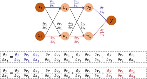
By adding the residual of PDEs/ODEs to the loss function, PDEs/ODEs can be cast into the loss function of PINNs and the final output can be constrained by the prior information. To calculate the residual of PDEs/ODEs in PINNs, it is necessary to compute the derivatives of network outputs with respect to the network inputs. This process can be achieved by using automatic differentiation (AD), which facilitates the development of PINN (Baydin, Pearlmutter, and Radul 2018). Unlike traditional numerical methods, AD can handle differential operators in a meshless way and does not differentiate data (Lu et al. 2021). To be specific, in the implementation of PINNs, AD can automatically calculate the derivatives of the neural network outputs with respect to the input variables, and this procedure is theoretically based on the chain rule. A simple feedforward neural network has been illustrated in Figure 2 to show how AD and the chain rule work. As shown in Figure 2, the input variables of the network are x₁ and x₂, and the output variable is y; v₁, v₂, v₃ and v₄ are the outputs of each neuron for each layer. The derivatives of y with respect to x₁ and x₂ can be calculated through the chain rule, as depicted in Figure 2. Some popular deep learning frameworks such as Tensorflow (Abadi et al. 2016) and Pytorch (Paszke et al. 2019) have effectively incorporated AD.

Figure 2. Illustration of implementing AD based on the chain rule (Rao, Sun, and Liu 2021).

3. Methodology and applications

3.1. Principles for solving forward and inverse problems

For PDEs with deterministic parameters, the aim of training a PINN is to obtain an accurate solution, which is regarded as the forward problem. Many research works have demonstrated the feasibility of using PINNs to obtain the solution of PDEs in forward problems (Raissi, Perdikaris, and Karniadakis 2017; Haghighat, Amini, and Juanes 2022; Niu et al. 2023). Abueidda, Lu, and Koric (2021) used PINNs to solve various boundary value problems (BVPs) containing different constitutive laws of solid materials. In this research, PINN was implemented as a PDE solver in a fairly straightforward manner. Different from conventional ML-based methods that rely on a large amount of data, this novel PINN-based paradigm can extract solutions from fully-understand physical laws with given initial and boundary conditions. Thus, when using PINNs to solve forward BVPs, accurate solutions can be obtained without resorting to data generation through numerical modelling software or laboratory tests (Rao, Sun, and Liu 2021; Abueidda, Lu, and Koric 2021; Sun et al. 2020; Zhu et al. 2019). The framework of using PINNs as a forward PDE solver is depicted in Figure 3(a). In this framework, there is no extra labelled data can be obtained except for initial and boundary conditions, and therefore the loss function only involves the loss value from initial conditions, boundary conditions and residuals of PDEs. If more data can be obtained when solving forward PDEs, the residual on data can also be incorporated into the loss function.

For most complex physics systems, the physics laws are partially known (Tartakovsky et al. 2018), and therefore the unknown parameters in equations should be identified first according to the observed data. PINN characterizes this kind of inverse problem (Cuomo et al. 2022; Lu et al. 2021; Raissi, Perdikaris, and Karniadakis 2019). One of the most outstanding advantages of PINNs is that they can solve inverse problems as easily as solving forward problems (Karniadakis et al. 2021; Lu et al. 2021; He et al. 2020; Raissi, Perdikaris, and Karniadakis 2019; Tartakovsky et al. 2020). Given the distinguished ability of PINNs to recover PDEs and solve PDEs, scholars have applied PINNs to various inverse problems in different domains, such as solid materials (Haghighat et al. 2021), supersonic flows (Jagtap et al. 2022), unknown diffusion coefficient estimation (Tartakovsky et al. 2018).

The framework for using PINNs to solve inverse problems is shown in Figure 3(b). Similarly, a general form of a PDE with unknown parameters can be described using the following equation (Raissi, Perdikaris, and Karniadakis 2019): (11) $u_t(t,\mathit{x})+\mathcal{D}[u(t,\mathit{x})\lambda ]=0,\mathit{x}\in \mathrm{\Omega },t\in [0,T]$(11) where $\lambda$ is the model parameter that needs to be identified. In this context, the unknown parameter is seen as a variable that would be updated during the training process, as shown in Figure 3(b). Similarly, the unknown parameter $\lambda$ and the variable u can be approximated by minimizing the MSE loss, which also contains the residual of data and the residual of PDEs: (12) $\begin{array}{rl}\mathcal{L}=& w_1\cdot \Vert u_t+\mathcal{D}[u\lambda ]{\Vert }_{\mathrm{\Omega }\times [0,T]}^2+w_2\cdot \\ & (\Vert u\text{–}{\mathcal{B}}_D(t\lambda ){\Vert }_{\mathrm{\partial }{\mathrm{\Omega }}_D\times [0,T]}^2+\Vert \mathbf{n}\cdot \mathrm{\nabla u}\text{–}{\mathcal{B}}_N(t\lambda ){\Vert }_{\mathrm{\partial }{\mathrm{\Omega }}_N\times [0,T]}^2)\\ & +w_3\cdot (\Vert u\text{–}{\mathcal{I}}_0(\mathit{x}\lambda ){\Vert }_{\mathrm{\Omega }\times [t=0]}^2+\Vert u_t\text{–}{\mathcal{I}}_1(\mathit{x}\lambda ){\Vert }_{\mathrm{\Omega }\times [t=0]}^2)\\ & +w_4\cdot \Vert u\text{–}{u}^{\ast }{\Vert }_{\mathrm{\Omega }\times [0,T]}^2\end{array}$(12) It should be noted that labelled data is indispensable for addressing inverse problems since there are unknown parameters that need to be identified.

3.2. Baseline neural networks

Before training, the underlying algorithm of PINNs is required to be determined based on the essence of the studied problem. Herein, three commonly used algorithms, fully-connected neural networks (FCNN), long short-term memory (LSTM) neural networks and convolutional neural networks (CNN) for building PINNs are introduced.

3.2.1. Fully-connected neural networks

The FCNN-based PINN models have prevailed over all PINN implementations (Cai, Wang, Wang, and Perdikaris 2021; Kharazmi, Zhang, and Karniadakis 2021; Jagtap et al. 2022). This FCNN-based PINN has been employed in various engineering domains, such as the multi-phase flow in porous media (Haghighat, Amini, and Juanes 2022), solid mechanics (Haghighat et al. 2021), surrogate modelling for fluid flows (Sun et al. 2020), geotechnical constitutive modelling (Zhang, Yin, and Sheil 2023a), and geotechnical hydromechanical modelling (Zhang et al. 2022). Generally, the prior information is embedded in the loss function of FCNN in the form of PDE/ODE residuals. The FCNN consists of the input, hidden and output layers. The hidden layers receive information from the input layer and pass the transformed information to the output layer. Supposing that the total number of hidden layers is L, this process can be described by using the following equations (Zhang, Yin, and Jin 2021): (13) $y_l={\sigma }_l({\mathbf{W}}_l{\mathit{y}}_{l-1}+{\mathit{b}}_l),l\in [1,L]$(13) (14) ${\mathit{y}}_{L+1}={\mathbf{W}}_{L+1}{\mathit{y}}_L+{\mathit{b}}_{L+1}$(14) where y_l is the output of the l^th layer and the input of the (l + 1)^th layer, W_l and b_l are the weight matrix and bias vector of the l^th layer, respectively, y₀ (l = 1) and y_L + 1 is the input and output of the FCNN, respectively, ${\sigma }_l$ is the activation function of each hidden layer.

During the training procedure, the parameters of the FCNN, W and b, are optimized gradually to minimize the discrepancy between the predictions and measurements. Finally, the output value y_L + 1 is generated as a prediction of the real value. The hyperparameters of the FCNN, such as the number of hidden layers and the number of neurons in each layer, should be tuned finely, which may have a significant impact on the convergence process and prediction accuracy (Cuomo et al. 2022). Especially when the data is sparse, which is a common case in PINN models, the network size affects the accuracy of the predictions significantly (He et al. 2020). To date, PINNs with FCNN architecture commonly determine the hyperparameters in a trial-and-error way (Raissi, Perdikaris, and Karniadakis 2019; Tartakovsky et al. 2020; He et al. 2020).

3.2.2. Long short-term memory neural network

LSTM neural networks (Hochreiter and Schmidhuber 1997) are also used to develop PINN-based models. LSTM is characterised by handling sequential data and dealing with long-time-lag tasks (Yang et al. 2019; Ma et al. 2022; Chen et al. 2023). As sequence-dependent problems are typical in the engineering domain, some attempts have been made to integrate physics into LSTM. For instance, Zhang, Liu, and Sun (2020) proposed a physics-informed multi-LSTM network. In this hybrid framework, two physics-informed multi-LSTM networks, e.g. phyLSTM² and phyLSTM³, are developed for modelling state space variables, restoring force, and hysteretic parameters. The physical laws are not only encoded in the network architecture but also embedded in the loss function. The proposed physics-informed models outperform purely data-driven models in terms of robustness, interpretability and generalizability. Zhang et al. (2022) proposed a physics-constrained LSTM to capture soil behaviour, in which the PDE-based constitutive laws are incorporated into the loss function to constrain the solution. The results demonstrated that this physics-constrained LSTM neural network surpassed traditional LSTM neural networks. Lahariya et al. (2022) also proposed physics-informed LSTM networks (PhyLSTMs) to model the evaporate cooling system, in which the residual of system dynamics is incorporated into the loss function. The authors also compare the performance of typical PINNs and PhyLSTMs, and the results demonstrated that PhyLSTMs can reach lower estimation errors and converge faster. To date, less research work focuses on the combination of PINNs with LSTM.

Overall, further research is expected to enhance the integration of conventional PINN frameworks with LSTM networks, with the aim of addressing a wider range of engineering problems with better performance and more flexibility.

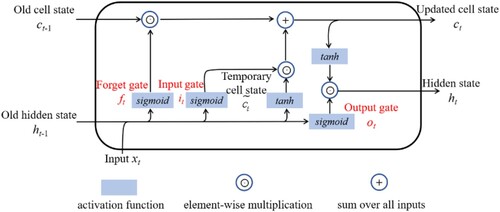
The basic building block of the LSTM is the memory cell, which has been illustrated in Figure 4. The information can be saved or forgotten by the memory cell, which is conducted by the input gate, forget gate and output gate, as shown (Hochreiter and Schmidhuber 1997): (15) $i_t=\sigma ({\mathbf{W}}_i\ast [{\mathit{h}}_{t-1},{\mathit{x}}_t]+{\mathit{b}}_i)$(15) (16) $f_t=\sigma ({\mathbf{W}}_f\ast [{\mathit{h}}_{t-1},{\mathit{x}}_t]+{\mathit{b}}_f)$(16) (17) $o_t=\sigma ({\mathbf{W}}_o\ast [{\mathit{h}}_{t-1},{\mathit{x}}_t]+{\mathit{b}}_o)$(17) where i_t, f_t, and o_t are the values of the input gate, forget gate and the output gate at the timestep t, respectively, $\sigma$ is the sigmoid function, W_i, W_f and W_o are the weight matrices of the input gate, forget gate and the output gate, respectively, h_t−1 is the hidden state at the timestep $t-1$, x_t is the input at the timestep t, b_i, b_f and b_o are the bias vectors of the input gate, forget gate and the output gate, respectively. Thereafter, the current cell state and the hidden state can be updated by using (Hochreiter and Schmidhuber 1997): (18) ${\tilde{c}}_t=\tanh ({\mathbf{W}}_c[{\mathit{h}}_{t-1},{\mathit{x}}_t]+{\mathit{b}}_c)$(18) (19) $c_t=i_t\odot {\tilde{c}}_t+f_t\odot c_{t-1}$(19) (20) ${\mathit{h}}_t=o_t\odot \tanh (c_t)$(20) where ${\tilde{c}}_t$ is the temporary cell state, tanh is the activation function, W_c and b_c are the weight matrix and the bias vector of the memory cell, respectively, c_t and c_t−1 are the updated cell state and the previous cell state, respectively, h_t is the updated hidden state, $\odot$ denotes for the element-wise multiplication. $i_t\odot {\tilde{c}}_t$ represents the selected information in the current timestep while $f_t\odot c_{t-1}$ represents the forgotten information from the previous timestep.

Figure 3. Framework of PINNs for (a) forward problems; and (b) inverse problems.

3.2.3. Convolutional neural network

CNN recently has also been used to construct a PINN-based model. CNN characterizes solving problems with large-scale spatio-temporal domains. Recently, scientists have made some attempts to incorporate physical constraints into CNNs, either in hard or soft manners. To embed hard constraints into the networks, the physical constraints should be encoded into the network architecture and design. In this way, the satisfaction of prior knowledge can be completely guaranteed. For instance, Kim et al. (2019) proposed a physics-informed CNN to conduct fluid simulations with divergence-free conditions to be hard-coded into the network. Similarly, Mohan et al. (2020) simulated three-dimensional turbulence with a physics-informed CNN, where the conservation laws and boundary conditions are strictly enforced all the time. Until now, many existing research works focus on using physical constraints in a soft manner in CNNs, by treating the physical constraints as penalty terms that are incorporated into loss functions in the form of PDE/ODE residuals (Gao, Sun, and Wang 2021; Sharma et al. 2018; Subramaniam et al. 2020; Wu et al. 2020). A standard CNN is limited to tackling regular geometries and uniform grids, while most scientific and engineering problems tend to have complex domains. Gao, Sun, and Wang (2021) used an elliptic coordinate mapping technique to transform an irregular solution domain into a regular domain, by which PDEs with irregular domains can be solved by CNNs.

The framework of CNN is shown in Figure 5. Generally, CNN consists of several convolutional, pooling and fully-connected layers. The size of the input image is denoted by h^r (height) × w^r (width) × c^r (channel, 1 for greyscale image and 3 for colour image). The convolutional layer is made of a series of filters or kernels, each having the same size of f × f. These filters or kernels slide on the input image from left to right and from top to bottom with a fixed stride s to extract specific features. This process is achieved by performing the element-wise multiplication between the filter matrix and the corresponding region of the input image. This region, termed the receptive field, matches the size of the filter. After convolved by n filters, the size of the input image is rescaled to h^c × w^c × c^c × n^c, and feature maps are generated for each filter subsequently. The size of the feature map can be determined by using the following equation (Zhang and Yin 2021): (21) $S_i^c=\lceil {\displaystyle \frac{S_i^r}{s}\rceil ,i=h,w}$(21) where $S_i^c$ and $S_i^r$ are the size of images along the i^th dimension in the convolutional and input layers, respectively, $\lceil \rceil$ is the ceiling function which maps x to the least integer larger than or equal to x.

Figure 4. Memory cell of an LSTM-based neural network (Yu et al. 2019).

The pooling layers are subsequently used to further reduce the number of parameters and dimensionality, and thus improve the training efficiency and prevent overfitting. The size of a h^c × w^c × c^c × n^c feature map is rescaled to h^p × w^p × c^p × n^c through the pooling layer. This process is achieved by replacing a specific area of the input image with a designated value, commonly the maximum value (Maximum Pooling) or the average value (Average Pooling). Finally, the outputs from the pooling layer are flattened and pass through a fully connected network to implement classification or regression tasks.

Overall, three different baseline neural networks are introduced in this section. The physics-informed FCNN can be used to model almost all scientific problems. This is because an FCNN with multiple hidden layers and proper training can approximate complicated functions or even any universal functions (Sun, Sengupta, and Juniper 2023). When solving sequence-based problems, using LSTM neural networks as an underlying architecture for PINNs is recommended. Additionally, when solving a problem with gridded two-dimensional or even high-dimensional datasets, physics-informed CNNs can be employed to reduce computational costs and improve training efficiency (Zhu et al. 2019).

4. Enhanced PINNs and applications

4.1. PINN variants

Based on the traditional forms of PINNs, numerous researchers focus on inventing various PINN variants to overcome their limitations and improve their performance. For instance, various domain segmentation methods combined with PINNs were proposed to solve complex problems with large spatial or time domains, as shown in Table 1. Meng et al. (2020) proposed a parareal physics-informed neural network (PPINN) for the long-time integration of time-dependent PDEs. In this framework, the long-time domain is decomposed into small sub-domains with the same interval. As the computational cost of conventional PINNs dealing with large data sets is prohibitively expensive, this approach can achieve significant speed-up and high computational efficiency by parallelly computing on small data sets. Similarly, Jagtap, Kharazmi, and Karniadakis (2020) proposed a conservative physics-informed neural network (cPINN) on discrete sub-domains. After obtaining every single solution for each separate sub-domain by using different PINN architectures, the final complete solution will be generated by patching every single solution together. This strategy takes advantage of network parallelization and therefore improves the training efficiency and breaks the curse of dimensionality. Furthermore, the domain segmentation method was further explored by Jagtap and Karniadakis (2021) and the extended physics-informed neural network (XPINN) was proposed to solve any type of PDEs. In this framework, the temporal and spatial domains can be decomposed in any arbitrary way. The error values on the interface are added to the loss function to ensure the continuity between subdomains. However, this framework somehow still fails to fulfill the continuity conditions on the interface due to the high-order derivatives in PDEs. The XPINN was further improved by Hu et al. (2022) as they extended it to the augmented physics-informed neural network (APINN). APINN employs a soft domain decomposition method. To be specific, the subdomains in APINN are characterized by continuous divisions rather than rigid boundaries. This is achieved by using gating networks, which are pre-trained and assign weights for subdomains. In this way, APINN does not incorporate intricate interface losses to preserve the continuity between subdomains.

Table 1. Various domain decomposition methods for PINNs.

PINN variants	Features	References
PPINN	Discrete the long-time domain	Meng et al. (2020)
cPINN	Decomposite the whole time-space domain; For nonlinear conservation laws	Jagtap, Kharazmi, and Karniadakis (2020)
XPINN	Discrete the domain arbitrarily; Applicable to any PDEs	Jagtap and Karniadakis (2021)
APINN	A soft-mannered decomposition method can be discovered through optimization	Hu et al. (2022)
hp-VPINN	The loss is presented in a variational form	Kharazmi, Zhang, and Karniadakis (2021); Kharazmi, Zhang, and Karniadakis (2019)

Another type of sub-domain method involves hp-variational forms of PINNs (hp-VPINNs) (Kharazmi, Zhang, and Karniadakis 2021, 2019). Each sub-domain is projected onto the space of high-order polynomials. By applying variational principles to Equation 1, the loss ${\mathcal{L}}^{({\mathrm{e}}_{\mathrm{x}}{\mathrm{e}}_{\mathrm{t}})}$ of each sub-domain ${\mathrm{\Omega }}_{{\mathrm{e}}_{\mathrm{x}}{\mathrm{e}}_{\mathrm{t}}}$ is presented in the form of integrals (Kharazmi, Zhang, and Karniadakis 2021): (22) ${\mathcal{R}}_{k_1{k}_2}^{(e_x{e}_t)}=\int \int (u_t(t,\mathit{x})+\mathcal{D}[u(t,\mathit{x})]){\varphi }_{k_1}^{(e_x)}{\varphi }_{k_2}^{(e_t)}\mathrm{d}{\mathrm{\Omega }}_{e_x{e}_t}$(22) (23) ${\mathcal{L}}^{(e_x{e}_t)}={\displaystyle \frac{1}{K_1{K}_2}{\sum }_{k=1}^{K_1{K}_2}{\Vert {\mathcal{R}}_{k_1{k}_2}^{(e_x{e}_t)}\Vert }^2}$(23) where ${\mathcal{R}}_{k_1{k}_2}^{(e_x{e}_t)}$ is the variational residual, ${\varphi }_{{\mathrm{k}}_1}^{({\mathrm{e}}_{\mathrm{x}})}$ and ${\varphi }_{{\mathrm{k}}_2}^{({\mathrm{e}}_{\mathrm{t}})}$ are the test functions of the size K₁ and K₂ in two dimensions, respectively. The integrals can be computed through numerical integration techniques such as Gauss quadrature rules. The training results demonstrate the superior performance of hp-VPINNs compared to classical PINNs when solving equations with non-smooth solutions characterized by singularities, steep solutions and sharp changes.

Apart from addressing general PDEs and ODEs, the traditional framework of PINNs is modified to solve multiple types of equations such as fractional equations (Pang, Lu, and Karniadakis 2019), nonlinear integro-differential equations (Yuan et al. 2022; Lu et al. 2021), interger-order PDEs (Raissi, Perdikaris, and Karniadakis 2019) and stochastic PDEs (Zhang, Guo, and Karniadakis 2020). Furthermore, integrating the Fourier feature into PINNs allows the network to approximate high-frequency functions in a low-dimensional domain (Tancik et al. 2020). Besides, to quantify the uncertainty of the generated results, the Bayesian framework can be combined with traditional PINNs, which are so-called BPINNs (Yang, Xuhui, and Karniadakis 2021). Overall, various PINN variants have been proposed to bypass the limitations of traditional PINNs and to improve their performance in solving complex problems involving different types of equations and uncertainty quantification.

4.2. Sampling methods

To ensure the effectiveness and accuracy of PINNs before the iterative training procedure, the training data should be sampled within the solution domain and at the edge of boundaries, using various sampling methods. An effective sampling strategy plays a fundamental role in ensuring the convergence of PINNs (Daw et al. 2023). Typically, current sampling can be classified into two categories: a fixed sampling method and an adaptive sampling method.

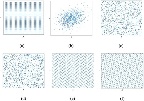
The fixed sampling strategy collects data points at the outset of training and keeps them the same throughout the training process. These selected data points can be uniformly or randomly distributed (Sun et al. 2020; Zhu et al. 2019). Regarding the randomly distributed data, various sampling methods including normal sampling, Latin hypercube sampling (Rao, Sun, and Liu 2021), Sobol' sequence (Pang, Lu, and Karniadakis 2019; Guo et al. 2022), Halton sequence and Hammersley sequence (Wu et al. 2023) have been used. Figure 6 shows their distributions.

Figure 5. Framework of convolutional neural network (Zhang and Yin 2021).

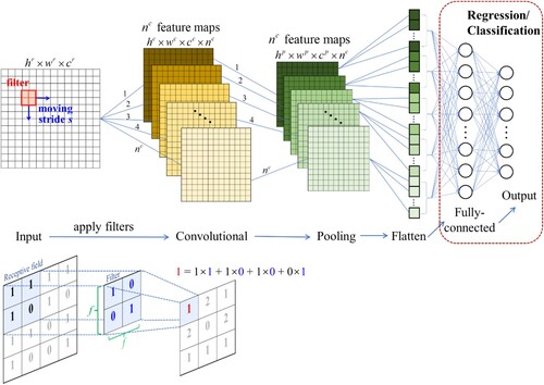
Figure 6. Fixed sampling methods: (a) uniform; (b) normal sampling; (c) Latin hypercube sampling; (d) Sobol' sequence; (e) Halton sequence; (f) Hammersley sequence.

Regarding the adaptive sampling method, a well-known strategy for optimizing the distribution of collocation points in each training epoch was presented by Lu et al. (2021), which is the so-called residual-based adaptive refinement (RAR) method. The RAR method works by continuously adding collocation points in regions where the PDE residual is relatively large until the mean residual is smaller than a threshold, which improves the training efficiency. More adaptive sampling methods have been proposed to enhance the training efficiency of PINNs (Sun, Sengupta, and Juniper 2023; Wu et al. 2023; Nabian, Gladstone, and Meidani 2021). The core of these strategies is to increase the density of training points in regions with poor predictions so that the trained model can better capture the underlying physics of problems. These adaptive sampling strategies were further improved by Retain-Resample-Release (R3) sampling method (Daw et al. 2023). The R3 method works by retaining training points in high residual regions, releasing training points that have been resolved, and maintaining a non-zero representation of points resampled from a uniform distribution over the entire domain. When the solution domain is very complex, adaptive sampling methods are recommended to improve the performance of PINNs.

4.3. Loss functions

Another crucial factor in obtaining an effective and accurate PINN model is the formulation of loss functions, which is still an open question in the study of PINNs. There are two commonly used types of loss functions in the field of computational mechanics: collocation point-based loss functions and energy-based loss functions. Most PINN models available in the literature enforce collocation point-based loss functions (Equations (6)–(10)), which are based on the strong form of PDEs. The training process aims to reduce the residuals of PDEs and initial/boundary conditions on each collocation point. Adam optimizer (Kingma and Ba 2014) and L-BFGS optimizer (Liu and Nocedal 1989) are generally applied to minimize the loss value. Apart from the widely adopted MSE for residual measurement, alternatives such as mean absolute error (MAE) have also been adopted. For instance, Rezaei et al. (2022) incorporate both MSE and MAE in the loss function when training PINNs, in order to keep the values of different loss terms in the same order. Despite the extensive applications of the collocation point-based loss function due to its simple and straightforward manner, it still has inherent limitations. These limitations can be summarized as: (1) The gradient pathologies are widely observed while the loss function has multiple residual terms and each term has different scales, thus resulting in a local minima solution rather than the global minima (Wang, Teng, and Perdikaris 2021; Elhamod et al. 2022); (2) The trained PINN model based on the collocation point residuals may lack generalization. While PINNs can generate accurate values on sampled collocation points, the error in the rest domain may be relatively large (Alzubaidi et al. 2021).

An alternative form of loss functions, known as energy-based loss functions is also employed in the training of PINNs. Unlike the conventional strong-form collocation point-based loss function, this approach is theoretically based on the weak form of PDEs, wherein the equilibrium equations and Neumann boundary conditions are implicitly incorporated into the loss function. One of the representative works of applying energy-based loss function in PINNs has been done by Samaniego et al. (2020). In this research, a so-called deep energy method (DEM) was proposed based on the principle of minimum potential energy. Specifically, the overall potential energy of the system is minimized when it reaches an equilibrium state, and this minimization process can be seen as an optimization problem which can be easily implemented by neural networks (Lanczos 2012). Therefore, the potential energy of the system can be used as the formulation of loss functions, which can be described by using the following equation (Samaniego et al. 2020): (24) $\mathcal{L}(u{)}_{\mathrm{energy}}=\mathrm{\Pi }(u)=U(u)\text{–}W(u)$(24) where $\mathit{\Pi }$ is the total system potential energy, $U$ indicates the internal energy and W indicates the external work. Samaniego et al. (2020) have successfully applied the proposed DEM method for displacement prediction of structures with linear elasticity, elastodynamics, and hyperelasticity constitutive models. He et al. (2023) later extended the DEM method to elastoplasticity problems for displacement prediction. The results demonstrate that by using the DEM instead of collocation point-based functions, the solutions are more accurate and gradient calculation is more efficient. Furthermore, an enhanced DEM method was proposed by Nguyen-Thanh et al. (2021), wherein the isoparametric element was integrated with DEM to transfer the irregular physical domain to a regular square domain. More implementations of formulating energy-based loss functions based on the principle of minimum potential energy can be found in Li, Bazant, and Zhu (2021) and Zhuang et al. (2021).

The energy-based loss function can also be formulated by using the variational energy of the system. Take the general form of a PDE in Equation 1 as an example, its energy function $\mathcal{E}(u)$ can be described by using (Goswami et al. 2020; Goswami et al. 2022): (25) $\mathcal{E}(u)=\int (\mathcal{g}[u_t(t,\mathit{x})+\mathcal{D}[u(t,\mathit{x})]])\mathrm{d}\mathrm{\Omega }$(25) where $\mathcal{g}$ is a differentiable function. It should be emphasized that all derivative terms in the $\mathcal{E}(u)$ can be efficiently and automatically calculated by AD.

In contrast to the computation of collocation point-based loss functions, the implementation of integrals is essential when computing energy-based loss functions. However, as it is almost impossible to analytically compute the complex integrals, the value of the integral should be approximated via various numerical integration methods, such as the Gauss quadrature rules (Kharazmi, Zhang, and Karniadakis 2019), the quasi-Monte Carlo integration (Morokoff and Caflisch 1995) and sparse grid quadratures (Smolyak 1963). Compared with conventional collocation point-based loss functions, energy-based loss functions have a lower order of derivatives, and therefore contribute to faster convergence (Goswami et al. 2020). Besides, the Neumann boundary condition and traction-free boundary condition can be automatically satisfied in the formulation of energy-based loss functions. However, the Dirichlet boundary conditions can only be exactly satisfied by modifying the output of the neural network (Goswami et al. 2020; Samaniego et al. 2020; Rezaei et al. 2022). The modification process could be challenging and intricate, particularly when dealing with complex or discontinuous boundary conditions. Li, Bazant, and Zhu (2021) also conducted a comparative analysis of collocation point-based and energy-based loss functions, evaluating the respective advantages and disadvantages of each. To date, more formulations of loss functions have been proposed, aiming at overcoming different difficulties when training PINNs. For instance, Fuhg and Bouklas (2022) proposed a mix-form of loss functions that combine the collocation point-based loss function with the energy-based loss function together. In this research, the collocation point-based loss function consists of residuals of governing equations and boundary conditions, and it was summed up with energy-based loss terms. By using this novel form of loss functions, the stress and displacement concentration features can be greatly resolved. Bai et al. (2023) also modified the loss function by using the least squares weighted residual method, and applied the modified framework for solving two-dimensional and three-dimensional solid mechanics problems. The training results showed that this modified loss function can predict both the displacement and stress field with accuracy and robustness.

4.4. Applications

In the field of geoengineering, extensive research has been done to investigate the feasibility of utilizing PINNs for geotechnical simulations. For instance, Bekele (2021) employed PINNs to successfully solve forward and inverse Terzaghi's one-dimensional consolidation problems. The application of PINNs for one-dimensional consolidation problems was further promoted by Zhang, Yin, and Sheil (2023b). This research systematically incorporated surcharge and vacuum loading conditions as boundary conditions. Furthermore, a Monte Carlo-based dropout uncertainty analysis was integrated into PINNs to effectively capture the inherent uncertainty characteristics of geotechnical problems. Another enhanced PINN model, the so-called affine physics–informed neural network (AfPINN) has also been proposed by Mandl et al. (2023) to solve consolidation problems. In this research, each output of the network should be rescaled by using scaling and offset factors, which can be understood as an affine transformation. In this case, the distribution of output variables can be tailored to be closer to the desired distribution. Besides, by scaling the gradient, the optimization process can be accelerated. When applying this AfPINN to the one-dimensional consolidation case, it generated more accurate results than conventional PINNs. The application of PINNs for simple consolidation problems was further expanded to more complex scenarios such as two-dimensionality (Lu and Mei 2022) or nonlinearity (Lan et al. 2023). PINNs have also been applied to modelling unsaturated flow in porous media. For instance, Depina et al. (2022) successfully employed PINNs to solve inverse groundwater flow problems modelled with the Richards partial differential equation and the vanGenuchten constitutive model. Haghighat, Amini, and Juanes (2022) also conducted a study on modelling unsaturated laminar flow in porous media, and they demonstrated that formulating the problem in the dimensionless form, along with a sequential training strategy and adaptive weighting methods significantly improved the stability of the PINN approach. Yang and Mei (2022) utilized PINNs to simulate the soil-water infiltration process, and the generated predictions agree with the numerical results. The applications of PINNs to other geotechnical problems have also been investigated, such as tunnelling (Zhang et al. 2023; Xu et al. 2023) and pile-soil interaction modelling (Vahab et al. 2023).

Overall, despite the great potential that PINNs have showcased, the applications of PINNs in the geotechnical domain are still sparse. Geoengineering problems are characterized by inherent complexity, and it is still challenging to accurately simulate complicated geoengineering problems through PINNs. More attention deserves to be paid to the geotechnical community.

5. Limitations and challenges

Despite the remarkable success that PINNs have achieved, there still exist limitations and challenges. One of the main challenges is modelling multiscale and multiphysics systems. Despite the outstanding success that PINNs have achieved in modelling complex systems (Lin et al. 2021; Liu and Wang 2021; Shin, Darbon, and Karniadakis 2020), it still requires tremendous investigations and development to improve the applicability of PINNs in engineering-scale problems. When modelling complex multiscale systems, the outputs of traditional PINNs may exhibit inaccuracies. Specifically, the networks excel in capturing low-frequency features whereas show weak performance in capturing high-frequency features (Rahaman et al. 2019; Leung, Lin, and Zhang 2022). When modelling multiphysics problems, the computational costs could be expensive to learn multiple physics parameters simultaneously (Karniadakis et al. 2021).

To better capture the high-frequency features in multiscale problems, some novel methods are proposed to address this issue. One of the most commonly used techniques is domain decomposition (Meng et al. 2020; Jagtap, Kharazmi, and Karniadakis 2020; Jagtap and Karniadakis 2021; Hu et al. 2022), which targets discretizing the time or space domain and calculating each sub-domain separately. Another efficient technique is passing the inputs through a Fourier feature mapping, which enables networks to learn high-frequency functions with fewer iterations (Tancik et al. 2020; Wang, Wang, and Perdikaris 2021). To better solve multiphysics problems with lower computational costs, using DeepM&Mnet is an effective way to construct complex models that can generate coupled solutions after learning each physics separately (Mao et al. 2021; Cai et al. 2021). The building block of this DeepM&Mnet framework is the DeepOnets, which is proposed by Lu et al. (2021) and is able to learn nonlinear functions accurately and effectively. Despite these advancements, we are still in the very early stages of tackling multiscale and multiphysics problems in engineering practice. Therefore, more novel techniques remain to be explored to improve the performance of PINNs in multiscale and multiphysics modelling.

Another challenge for PINNs is their performance in dealing with complex constitutive models, particularly in the geotechnical domain. Soils are characterized by various complex behaviours including multiphysics coupling (Yang et al. 2019), high dimensionality (Bi et al. 2021), anisotropy (Yin et al. 2010), non-coaxiality (Tian and Yao 2017), stress dilatancy (He et al. 2022), time-dependence (Wang et al. 2018), stress-path dependence (Chang and Zhang 2013). An attempt to apply PINNs to elastoplastic models has been made by Haghighat et al. (2021), and the authors pointed out that standard physics-constrained multi-layer neural networks may fail to capture localised deformation in elastoplastic problems. Haghighat, Abouali, and Vaziri (2023) also proposed an elastoplastic PDE solver to deal with constitutive models. However, this PDE solver was only validated in uniaxial and biaxial loading conditions. While the real loading condition in nature is much more complex, the effectiveness of the proposed methodology may not be guaranteed under more complex conditions. Moreover, simulating constitutive relations always requires a large amount of strain-stress data, especially when the complexity of constitutive relations increases. To better modelling constitutive relations without resorting to deeper and wider PINNs, as well as prevent the need for a large dataset, the multi-fidelity residual framework has been integrated with PINNs (Zhang, Yin, and Sheil 2023a; Zhang et al. 2022). Besides, some successful trials of utilizing PINNs for modelling soil behaviours have been done, including path-dependent behaviour (Zhang et al. 2022), through which the potential of PINNs to capture complex soil behaviours is demonstrated. However, this topic of research still has a limited number of available studies.

Actually, the fundamental obstacle underlying the aforementioned problems is the convergence issue. Given that most physics-informed learning involves minimizing complicated loss functions that have multiple loss terms, there would be non-convex optimization difficulties and therefore leading to the instability of the training process and convergence to local minima or saddle points (Karniadakis et al. 2021; Lee et al. 2016; Blum and Rivest 1992). For example, Wang, Yu, and Perdikaris (2022) employed a PINN to solve a nonlinear hyperbolic transport PDE with a non-convex flux function. In this work, the neural network completely fails to identify the exact solution. Researchers have been endeavouring to improve convergence by optimizing the architecture of neural networks or using adaptive activation functions (Jagtap, Kawaguchi, and Karniadakis 2020; Jagtap, Kawaguchi, and Karniadakis 2020; Wang, Teng, and Perdikaris 2021). Additionally, to mitigate the imbalance of different loss terms to the total loss, a self-adaptive loss balancing strategy was tailored to achieve higher accuracy and better convergence (Xiang et al. 2022; Anagnostopoulos, Toscano, and Stergiopulos 2023). Another example is to use curriculum regularization or pose the problem as a sequence-to-sequence learning task to alleviate the optimization difficulties (Wang, Yu, and Perdikaris 2022). While significant progress has been made in developing convergence acceleration strategies for PINNs, there is a growing need to investigate more flexible optimization methods to improve the stability of PINNs. A key issue of this endeavour invloves digging out more theoretical relationships between optimization or acceleration algorithms and the performance of PINNs.

6. Conclusions

This study provided a comprehensive review of the current state of physics-informed neural networks (PINNs), which provides an alternative solver for deriving solutions of partial differential equations (PDEs). Firstly, the framework for employing PINNs in solving forward and inverse PDEs was introduced, followed by an elaboration of three baseline neural networks including fully-connected neural networks (FCNN), long short-term memory (LSTM) neural networks and convolutional neural networks (CNN) used for developing PINNs. Then, some novel strategies that focus on improving the performance of PINNs were introduced from three aspects: PINN variants, sampling methods including fixed and adaptive sampling strategy, and loss functions involving collocation point-based and energy-based formulations. Finally, the limitations and challenges of current PINNs were summarized. The main conclusions are made as follows:

1. FCNN is still the predominant choice for training PINNs and it has been widely used in engineering practice. The LSTM neural network characterizes handling sequence-based problems and CNN exhibits great potential to solve problems with large-scale spatial-temporal domains or high-dimensionality. Further research is anticipated to explore the integration of PINNs with various neural networks, enabling PINNs to tackle a broader spectrum of engineering problems.

2. Various domain decomposition methods have been proposed to improve the training efficiency of PINNs and bypass the curse of dimensionality when dealing with large and complex domains. Two representative models are the extended physics-informed neural network (XPINN) and the hp-variational physics-informed neural network (hp-VPINN). XPINN can be used to discrete domain arbitrarily and therefore has been used to solve any type of PDEs. hp-VPINN presents the loss in each subdomain in a variational form and showcases their accuracy and effectiveness when tackling non-smooth functions.

3. Two sampling methods, fixed sampling and adaptive sampling are compared. Fixed sampling methods, characterized by keeping training datasets unchanged throughout the training procedure, dominate the application of sampling in PINNs due to their simplicity. However, in the context of solving complex problems in which convergence problems may occur, adaptive sampling methods are recommended.

4. The framework of two types of loss functions is introduced and compared in this study. The collocation point-based loss functions, which incorporate residuals of PDEs/ODEs, measured data, and initial/boundary conditions in sampled points, are widely adopted when training PINNs. On the other hand, the energy-based loss functions, characterized by their relatively lower order of derivatives, have exhibited superior performance to traditional collocation point-based loss functions in terms of faster convergence, but energy-based loss functions have been rarely used. Therefore, further research efforts are expected to investigate the applicability and effectiveness of using energy-based loss functions or even more formulations of loss functions in PINNs.

5. Current PINNs still encounter challenges when addressing complex systems, including multiscale or multiphysics problems, as well as modelling complex constitutive relations. Although some trials have been made to overcome limitations, most of these trials are still limited to simple nonlinear functions (e.g. low dimensional and single phase) and their applicability to engineering-scale problems may not be guaranteed. These limitations primarily stem from poor convergence. In order to prompt the application of PINNs and prove their significance in solving practical problems, there is a need for the development of additional learning algorithms that target enhancing convergence and accelerating the optimization process.

Disclosure statement

No potential conflict of interest was reported by the author(s).

Data availability statement

All data that support the findings of this study are available from the corresponding author upon reasonable request.

Correction Statement

This article has been corrected with minor changes. These changes do not impact the academic content of the article.

Additional information

Funding

This work was supported by Hong Kong Polytechnic University; Research Grants Council (RGC) of the Hong Kong Special Administrative Region Government (HKSARG) of China: [grant number 15220221; 15229223]; Royal Society under the Newton International Fellowship.

References

- Abadi, M., P. Barham, J. Chen, Z. Chen, A. Davis, J. Dean, M. Devin, S. Ghemawat, G. Irving, and M. Isard. 2016. “TensorFlow: A System for Large-Scale Machine Learning.” 12th USENIX Symposium on Operating Systems Design and Implementation (OSDI 16), 265–283.
- Abueidda, D. W., S. Koric, R. A. Al-Rub, C. M. Parrott, K. A. James, and N. A. Sobh. 2022. “A Deep Learning Energy Method for Hyperelasticity and Viscoelasticity.” European Journal of Mechanics-A/Solids 95: 104639. https://doi.org/10.1016/j.euromechsol.2022.104639.
- Abueidda, D. W., Q. Lu, and S. Koric. 2021. “Meshless Physics-Informed Deep Learning Method for Three-Dimensional Solid Mechanics.” International Journal for Numerical Methods in Engineering 122 (23): 7182–7201. https://doi.org/10.1002/nme.6828.
- Alzubaidi, L., J. Zhang, A. J. Humaidi, A. Al-Dujaili, Y. Duan, O. Al-Shamma, J. Santamaría, M. A. Fadhel, M. Al-Amidie, and L. Farhan. 2021. “Review of Deep Learning: Concepts, CNN Architectures, Challenges, Applications, Future Directions.” Journal of big Data 8: 1–74. https://doi.org/10.1186/s40537-021-00444-8.
- Anagnostopoulos, S. J., J. D. Toscano, and N. Stergiopulos. 2023. “Residual-Based Attention and Connection to Information Bottleneck Theory in PINNs.” arXiv preprint arXiv:2307.00379, 2023.
- Asaoka, A. 1978. “Observational Procedure of Settlement Prediction.” Soils and Foundations 18 (4): 87–101. https://doi.org/10.3208/sandf1972.18.4_87.
- Bai, J., T. Rabczuk, A. Gupta, L. Alzubaidi, and Y. Gu. 2023. “A Physics-Informed Neural Network Technique Based on a Modified Loss Function for Computational 2D and 3D Solid Mechanics.” Computational Mechanics 71 (3): 543–562. https://doi.org/10.1007/s00466-022-02252-0.
- Baydin, A., B. Pearlmutter, and A. Radul. 2018. “Automatic Differentiation in Machine Learning: A Survey.” Journal of Marchine Learning Research 18: 1–43.
- Bekele, Y. W. 2021. “Physics-informed Deep Learning for One-Dimensional Consolidation.” Journal of Rock Mechanics and Geotechnical Engineering 13 (2): 420–430. https://doi.org/10.1016/j.jrmge.2020.09.005.
- Bi, J., H. Zhang, X. Luo, H. Shen, and Z. Li. 2021. “Modeling of Internal Erosion Using Particle Size as an Extra Dimension.” Computers and Geotechnics 133. https://doi.org/10.1016/j.compgeo.2021.104021.
- Bishop, C. M., and N. M. Nasrabadi. 2006. Pattern Recognition and Machine Learning. Vol. 4. New York: Springer .
- Blum, A. L., and R. L. Rivest. 1992. “Training a 3-Node Neural Network is NP-Complete.” Neural Networks 5 (1): 117–127. https://doi.org/10.1016/S0893-6080(05)80010-3.
- Cai, S., Z. Mao, Z. Wang, M. Yin, and G. E. Karniadakis. 2022. “Physics-informed Neural Networks (PINNs) for Fluid Mechanics: A Review.” Acta Mechanica Sinica 37 (12): 1727–1738. https://doi.org/10.1007/s10409-021-01148-1.
- Cai, S., Z. Wang, C. Chryssostomidis, and G. E. Karniadakis. 2020. “Heat Transfer Prediction with Unknown Thermal Boundary Conditions using Physics-Informed Neural Networks.” In Fluids Engineering Division Summer Meeting, V003T05A54. American Society of Mechanical Engineers.
- Cai, S., Z. Wang, L. Lu, T. A. Zaki, and G. E. Karniadakis. 2021. “DeepM&Mnet: Inferring the Electroconvection Multiphysics Fields Based on Operator Approximation by Neural Networks.” Journal of Computational Physics 436. https://doi.org/10.1016/j.jcp.2021.110296.
- Cai, S., Z. Wang, S. Wang, P. Perdikaris, and G. E. Karniadakis. 2021. “Physics-Informed Neural Networks for Heat Transfer Problems.” Journal of Heat Transfer 143 (6), https://doi.org/10.1115/1.4050542.
- Chang, D. S., and L. M. Zhang. 2013. “Critical Hydraulic Gradients of Internal Erosion Under Complex Stress States.” Journal of Geotechnical and Geoenvironmental Engineering 139 (9): 1454–1467. https://doi.org/10.1061/(asce)gt.1943-5606.0000871.
- Chen, X. X., J. Yang, G. F. He, and L. C. Huang. 2023. “Development of an LSTM-Based Model for Predicting the Long-Term Settlement of Land Reclamation and a GUI-Based Tool.” Acta Geotechnica 18 (1): 1–14. https://doi.org/10.1007/s11440-022-01579-5.
- Cividini, A., and G. Gioda. 2004. “Finite-Element Approach to the Erosion and Transport of Fine Particles in Granular Soils.” International Journal of Geomechanics 4 (3): 191–198. https://doi.org/10.1061/(ASCE)1532-3641(2004)4:3(191).
- Cuomo, S., V. S. d. Cola, F. Giampaolo, G. Rozza, M. Raissi, and F. Piccialli. 2022. “Scientific Machine Learning through Physics-Informed Neural Networks: Where we are and What’s next.” arXiv:2201.05624.
- Daolun, L., S. Luhang, Z. Wenshu, L. Xuliang, and T. Jieqing. 2021. “Physics-constrained Deep Learning for Solving Seepage Equation.” Journal of Petroleum Science and Engineering 206. https://doi.org/10.1016/j.petrol.2021.109046.
- Davi, C., and U. Braga-Neto. 2022. “Pso-pinn: Physics-informed Neural Networks Trained with Particle Swarm Optimization.” arXiv preprint arXiv:2202.01943.
- Daw, A., J. Bu, S. Wang, P. Perdikaris, and A. Karpatne. 2023. “Mitigating Propagation Failures in Physics-informed Neural Networks using Retain-Resample-Release (R3) Sampling”.
- Depina, I., S. Jain, S. Mar Valsson, and H. Gotovac. 2022. “Application of Physics-Informed Neural Networks to Inverse Problems in Unsaturated Groundwater Flow.” Georisk: Assessment and Management of Risk for Engineered Systems and Geohazards 16 (1): 21–36. https://doi.org/10.1080/17499518.2021.1971251.
- Diao, Y., J. Yang, Y. Zhang, D. Zhang, and Y. Du. 2023. “Solving Multi-Material Problems in Solid Mechanics Using Physics-Informed Neural Networks Based on Domain Decomposition Technology.” Computer Methods in Applied Mechanics and Engineering 413: 116120. https://doi.org/10.1016/j.cma.2023.116120.
- Earij, A., G. Alfano, K. Cashell, and X. Zhou. 2017. “Nonlinear Three–Dimensional Finite–Element Modelling of Reinforced–Concrete Beams: Computational Challenges and Experimental Validation.” Engineering Failure Analysis 82: 92–115. https://doi.org/10.1016/j.engfailanal.2017.08.025.
- Elhamod, M., J. Bu, C. Singh, M. Redell, A. Ghosh, V. Podolskiy, W.-C. Lee, and A. Karpatne. 2022. “CoPhy-PGNN: Learning Physics-Guided Neural Networks with Competing Loss Functions for Solving Eigenvalue Problems.” ACM Transactions on Intelligent Systems and Technology 13 (6): 1–23. https://doi.org/10.1145/3530911.
- Feng, J. X., P. P. Ni, and G. X. Mei. 2019. “One-Dimensional Self-Weight Consolidation with Continuous Drainage Boundary Conditions: Solution and Application to Clay-Drain Reclamation.” International Journal for Numerical and Analytical Methods in Geomechanics 43 (8): 1634–1652. https://doi.org/10.1002/nag.2928.
- Feyel, F. 2003. “A Multilevel Finite Element Method (FE2) to Describe the Response of Highly non-Linear Structures Using Generalized Continua.” Computer Methods in Applied Mechanics and Engineering 192 (28-30): 3233–3244. https://doi.org/10.1016/s0045-7825(03)00348-7.
- Fuhg, J. N., and N. Bouklas. 2022. “The Mixed Deep Energy Method for Resolving Concentration Features in Finite Strain Hyperelasticity.” Journal of Computational Physics 451: 110839. https://doi.org/10.1016/j.jcp.2021.110839.
- Gao, H., L. Sun, and J. X. Wang. 2021. “PhyGeoNet: Physics-Informed Geometry-Adaptive Convolutional Neural Networks for Solving Parameterized Steady-State PDEs on Irregular Domain.” Journal of Computational Physics 428. https://doi.org/10.1016/j.jcp.2020.110079.
- Geers, M. G., V. G. Kouznetsova, K. Matouš, and J. Yvonnet. 2017. “Homogenization Methods and Multiscale Modeling: Nonlinear Problems.” Encyclopedia of Computational Mechanics Second Edition, 1–34.
- Goodfellow, I., Y. Bengio, and A. Courville. 2016. Deep Learning. MIT press.
- Goswami, S., C. Anitescu, S. Chakraborty, and T. Rabczuk. 2020. “Transfer Learning Enhanced Physics Informed Neural Network for Phase-Field Modeling of Fracture.” Theoretical and Applied Fracture Mechanics 106: 102447. https://doi.org/10.1016/j.tafmec.2019.102447.
- Goswami, S., M. Yin, Y. Yu, and G. E. Karniadakis. 2022. “A Physics-Informed Variational DeepONet for Predicting Crack Path in Quasi-Brittle Materials.” Computer Methods in Applied Mechanics and Engineering 391: 114587. https://doi.org/10.1016/j.cma.2022.114587.
- Guo, H., X. Zhuang, P. Chen, N. Alajlan, and T. Rabczuk. 2022. “Analysis of Three-Dimensional Potential Problems in Non-Homogeneous Media with Physics-Informed Deep Collocation Method Using Material Transfer Learning and Sensitivity Analysis.” Engineering with Computers 38 (6): 5423–5444. https://doi.org/10.1007/s00366-022-01633-6.
- Haghighat, E., S. Abouali, and R. Vaziri. 2023. “Constitutive Model Characterization and Discovery Using Physics-Informed Deep Learning.” Engineering Applications of Artificial Intelligence 120. https://doi.org/10.1016/j.engappai.2023.105828.
- Haghighat, E., D. Amini, and R. Juanes. 2022. “Physics-informed Neural Network Simulation of Multiphase Poroelasticity Using Stress-Split Sequential Training.” Computer Methods in Applied Mechanics and Engineering 397. https://doi.org/10.1016/j.cma.2022.115141.
- Haghighat, E., M. Raissi, A. Moure, H. Gomez, and R. Juanes. 2021. “A Physics-Informed Deep Learning Framework for Inversion and Surrogate Modeling in Solid Mechanics.” Computer Methods in Applied Mechanics and Engineering 379. https://doi.org/10.1016/j.cma.2021.113741.
- He, J., D. Abueidda, R. A. Al-Rub, S. Koric, and I. Jasiuk. 2023. “A Deep Learning Energy-Based Method for Classical Elastoplasticity.” International Journal of Plasticity 162: 103531. https://doi.org/10.1016/j.ijplas.2023.103531.
- He, Q., D. Barajas-Solano, G. Tartakovsky, and A. M. Tartakovsky. 2020. “Physics-informed Neural Networks for Multiphysics Data Assimilation with Application to Subsurface Transport.” Advances in Water Resources 141. https://doi.org/10.1016/j.advwatres.2020.103610.
- He, S. H., D. Zhi, Y. Sun, M. Goudarzy, and W. Y. Chen. 2022. “Stress–Dilatancy Behavior of Dense Marine Calcareous Sand Under High-Cycle Loading: An Experimental Investigation.” Ocean Engineering 244: 110437. https://doi.org/10.1016/j.oceaneng.2021.110437.
- Ho, L., and B. Fatahi. 2016. “One-Dimensional Consolidation Analysis of Unsaturated Soils Subjected to Time-Dependent Loading.” International Journal of Geomechanics 16 (2), https://doi.org/10.1061/(asce)gm.1943-5622.0000504.
- Hochreiter, S., and J. Schmidhuber. 1997. “Long Short-Term Memory.” Neural Computation 9 (8): 1735–1780. https://doi.org/10.1162/neco.1997.9.8.1735.
- Hu, Z., A. D. Jagtap, G. E. Karniadakis, and K. Kawaguchi. 2022. “Augmented Physics-Informed Neural Networks (APINNs): A Gating Network-Based Soft Domain Decomposition Methodology.” arXiv:2211.08939.
- Jagtap, A. D., and G. E. Karniadakis. 2021. “Extended Physics-informed Neural Networks (XPINNs): A Generalized Space-Time Domain Decomposition based Deep Learning Framework for Nonlinear Partial Differential Equations.” AAAI Spring Symposium: MLPS.
- Jagtap, A. D., K. Kawaguchi, and G. E. Karniadakis. 2020. “Adaptive Activation Functions Accelerate Convergence in Deep and Physics-Informed Neural Networks.” Journal of Computational Physics 404. https://doi.org/10.1016/j.jcp.2019.109136.
- Jagtap, A. D., K. Kawaguchi, and G. Em Karniadakis. 2020. “Locally Adaptive Activation Functions with Slope Recovery for Deep and Physics-Informed Neural Networks.” Proceedings of the Royal Society A: Mathematical, Physical and Engineering Sciences 476 (2239): 20200334. https://doi.org/10.1098/rspa.2020.0334.
- Jagtap, A. D., E. Kharazmi, and G. E. Karniadakis. 2020. “Conservative Physics-Informed Neural Networks on Discrete Domains for Conservation Laws: Applications to Forward and Inverse Problems.” Computer Methods in Applied Mechanics and Engineering 365. https://doi.org/10.1016/j.cma.2020.113028.
- Jagtap, A. D., Z. Mao, N. Adams, and G. E. Karniadakis. 2022. “Physics-informed Neural Networks for Inverse Problems in Supersonic Flows.” Journal of Computational Physics 466. https://doi.org/10.1016/j.jcp.2022.111402.
- Jin, X., S. Cai, H. Li, and G. E. Karniadakis. 2021. “NSFnets (Navier-Stokes Flow Nets): Physics-Informed Neural Networks for the Incompressible Navier-Stokes Equations.” Journal of Computational Physics 426. https://doi.org/10.1016/j.jcp.2020.109951.
- Karniadakis, G. E., I. G. Kevrekidis, L. Lu, P. Perdikaris, S. Wang, and L. Yang. 2021. “Physics-informed Machine Learning.” Nature Reviews Physics 3 (6): 422–440. https://doi.org/10.1038/s42254-021-00314-5.
- Kharazmi, E., Z. Zhang, and G. E. Karniadakis. 2019. “Variational Physics-informed Neural Networks for Solving Partial Differential Equations.” arXiv preprint arXiv:1912.00873.
- Kharazmi, E., Z. Zhang, and G. E. Karniadakis. 2021. “hp-VPINNs: Variational Physics-Informed Neural Networks with Domain Decomposition.” Computer Methods in Applied Mechanics and Engineering 374: 113547. https://doi.org/10.1016/j.cma.2020.113547.
- Kim, B., V. C. Azevedo, N. Thuerey, T. Kim, M. Gross, and B. Solenthaler. 2019. “Deep Fluids: A Generative Network for Parameterized Fluid Simulations.” In Computer Graphics Forum, 59–70. Wiley Online Library.
- Kim, J., K. Lee, D. Lee, S. Y. Jhin, and N. Park. 2021. Year of Conference. “DPM: A Novel Training Method for Physics-Informed Neural Networks in Extrapolation.”.” Proceedings of the AAAI Conference on Artificial Intelligence 35 (9): 8146–8154. https://doi.org/10.1609/aaai.v35i9.16992.
- Kingma, D. P., and J. Ba. 2014. “Adam: A Method for Stochastic Optimization.” Proceedings of International Conference on Learning Representations.
- Lagaris, I. E., A. Likas, and D. I. Fotiadis. 1998. “Artificial Neural Networks for Solving Ordinary and Partial Differential Equations.” IEEE Transactions on Neural Networks 9 (5): 987–1000. https://doi.org/10.1109/72.712178.
- Lahariya, M., F. Karami, C. Develder, and G. Crevecoeur. 2022. “Physics-Informed LSTM Network for Flexibility Identification in Evaporative Cooling System.” IEEE Transactions on Industrial Informatics 19 (2): 1484–1494. https://doi.org/10.1109/TII.2022.3173897.
- Lan, P., J.-j Su, X.-y. Ma, and S. Zhang. 2023. “Application of Improved Physics-Informed Neural Networks for Nonlinear Consolidation Problems with Continuous Drainage Boundary Conditions.” Acta Geotechnica 19 (1): 495–508. https://doi.org/10.1007/s11440-023-01899-0.
- Lanczos, C. 2012. The Variational Principles of Mechanics. Courier Corporation.
- Lee, H., and I. S. Kang. 1990. “Neural Algorithm for Solving Differential Equations.” Journal of Computational Physics 91 (1): 110–131. https://doi.org/10.1016/0021-9991(90)90007-N.
- Lee, J. D., M. Simchowitz, M. I. Jordan, and B. Recht. 2016. “Gradient Descent Only Converges to Minimizers.” Conference on Learning Theory, 1246–1257.
- Leung, W. T., G. Lin, and Z. Zhang. 2022. “NH-PINN: Neural Homogenization-Based Physics-Informed Neural Network for Multiscale Problems.” Journal of Computational Physics 470. https://doi.org/10.1016/j.jcp.2022.111539.
- Li, W., M. Z. Bazant, and J. Zhu. 2021. “A Physics-Guided Neural Network Framework for Elastic Plates: Comparison of Governing Equations-Based and Energy-Based Approaches.” Computer Methods in Applied Mechanics and Engineering 383. https://doi.org/10.1016/j.cma.2021.113933.
- Lin, C., Z. Li, L. Lu, S. Cai, M. Maxey, and G. E. Karniadakis. 2021. “Operator Learning for Predicting Multiscale Bubble Growth Dynamics.” The Journal of Chemical Physics 154 (10): 104118. https://doi.org/10.1063/5.0041203.
- Liu, D. C., and J. Nocedal. 1989. “On the Limited Memory BFGS Method for Large Scale Optimization.” Mathematical Programming 45 (1-3): 503–528. https://doi.org/10.1007/BF01589116.
- Liu, X., S. Tian, F. Tao, and W. Yu. 2021. “A Review of Artificial Neural Networks in the Constitutive Modeling of Composite Materials.” Composites Part B: Engineering 224. https://doi.org/10.1016/j.compositesb.2021.109152.
- Liu, D., and Y. Wang. 2019. “Multi-fidelity Physics-Constrained Neural Network and Its Application in Materials Modeling.” Journal of Mechanical Design 141 (12): 121403. https://doi.org/10.1115/1.4044400.
- Liu, D., and Y. Wang. 2021. “A Dual-Dimer Method for Training Physics-Constrained Neural Networks with Minimax Architecture.” Neural Networks 136: 112–125. https://doi.org/10.1016/j.neunet.2020.12.028.
- Lu, L., P. Jin, G. Pang, Z. Zhang, and G. E. Karniadakis. 2021. “Learning Nonlinear Operators via DeepONet Based on the Universal Approximation Theorem of Operators.” Nature Machine Intelligence 3 (3): 218–229. https://doi.org/10.1038/s42256-021-00302-5.
- Lu, Y., and G. Mei. 2022. “A Deep Learning Approach for Predicting two-Dimensional Soil Consolidation Using Physics-Informed Neural Networks (Pinn).” Mathematics 10 (16): 2949. https://doi.org/10.3390/math10162949.
- Lu, L., X. Meng, Z. Mao, and G. E. Karniadakis. 2021. “DeepXDE: A Deep Learning Library for Solving Differential Equations.” SIAM Review 63 (1): 208–228. https://doi.org/10.1137/19M1274067.
- Ma, K., L. P. Chen, Q. Fang, and X. F. Hong. 2022. “Machine Learning in Conventional Tunnel Deformation in High in Situ Stress Regions.” Symmetry 14 (3. https://doi.org/10.3390/sym14030513.
- Ma, B. H., Z. Y. Hu, Z. Li, K. Cai, M. H. Zhao, C. B. He, and X. C. Huang. 2020. “Finite Difference Method for the One-Dimensional Non-Linear Consolidation of Soft Ground Under Uniform Load.” Frontiers in Earth Science 8. https://doi.org/10.3389/feart.2020.00111.
- Mandl, L., A. Mielke, S. M. Seyedpour, and T. Ricken. 2023. “Affine Transformations Accelerate the Training of Physics-Informed Neural Networks of a one-Dimensional Consolidation Problem.” Scientific Reports 13 (1): 15566. https://doi.org/10.1038/s41598-023-42141-x.
- Mao, Z., A. D. Jagtap, and G. E. Karniadakis. 2020. “Physics-informed Neural Networks for High-Speed Flows.” Computer Methods in Applied Mechanics and Engineering 360. https://doi.org/10.1016/j.cma.2019.112789.
- Mao, Z., L. Lu, O. Marxen, T. A. Zaki, and G. E. Karniadakis. 2021. “DeepM&Mnet for Hypersonics: Predicting the Coupled Flow and Finite-Rate Chemistry Behind a Normal Shock Using Neural-Network Approximation of Operators.” Journal of Computational Physics 447. https://doi.org/10.1016/j.jcp.2021.110698.
- McClenny, L., and U. Braga-Neto. 2020. “Self-adaptive Physics-informed Neural Networks using a Soft Attention Mechanism.” arXiv preprint arXiv:2009.04544.
- Meng, X., Z. Li, D. Zhang, and G. E. Karniadakis. 2020. “PPINN: Parareal Physics-Informed Neural Network for Time-Dependent PDEs.” Computer Methods in Applied Mechanics and Engineering 370. https://doi.org/10.1016/j.cma.2020.113250.
- Mohan, A. T., N. Lubbers, D. Livescu, and M. Chertkov. 2020. “Embedding Hard Physical Constraints in Neural Network Coarse-Graining of 3D Turbulence.” arXiv preprint arXiv:2002.00021.
- Monaghan, J. J. 1992. “Smoothed Particle Hydrodynamics.” Annual Review of Astronomy and Astrophysics 30 (1): 543–574. https://doi.org/10.1146/annurev.aa.30.090192.002551.
- Morokoff, W. J., and R. E. Caflisch. 1995. “Quasi-monte Carlo Integration.” Journal of Computational Physics 122 (2): 218–230. https://doi.org/10.1006/jcph.1995.1209.
- Nabian, M. A., R. J. Gladstone, and H. Meidani. 2021. “Efficient Training of Physics-Informed Neural Networks via Importance Sampling.” Computer-Aided Civil and Infrastructure Engineering 36 (8): 962–977. https://doi.org/10.1111/mice.12685.
- Nguyen-Thanh, V. M., C. Anitescu, N. Alajlan, T. Rabczuk, and X. Zhuang. 2021. “Parametric Deep Energy Approach for Elasticity Accounting for Strain Gradient Effects.” Computer Methods in Applied Mechanics and Engineering 386: 114096. https://doi.org/10.1016/j.cma.2021.114096.
- Niu, S., E. Zhang, Y. Bazilevs, and V. Srivastava. 2023. “Modeling Finite-Strain Plasticity Using Physics-Informed Neural Network and Assessment of the Network Performance.” Journal of the Mechanics and Physics of Solids 172. https://doi.org/10.1016/j.jmps.2022.105177.
- Pang, G., L. Lu, and G. E. Karniadakis. 2019. “fPINNs: Fractional Physics-Informed Neural Networks.” SIAM Journal on Scientific Computing 41 (4): A2603–A2A26. https://doi.org/10.1137/18m1229845.
- Paszke, A., S. Gross, F. Massa, A. Lerer, J. Bradbury, G. Chanan, T. Killeen, Z. Lin, N. Gimelshein, and L. Antiga. 2019. “Pytorch: An Imperative Style, High-Performance Deep Learning Library.” Advances in Neural Information Processing Systems 32.
- Psichogios, D. C., and L. H. Ungar. 1992. “A Hybrid Neural Network-First Principles Approach to Process Modeling.” AIChE Journal 38 (10): 1499–1511. https://doi.org/10.1002/aic.690381003.
- Rahaman, N., A. Baratin, D. Arpit, F. Draxler, M. Lin, F. Hamprecht, Y. Bengio, and A. Courville. 2019. “On the Spectral Bias of Neural Networks.” International Conference on Machine Learning, 5301–5310.
- Raissi, M., P. Perdikaris, and G. E. Karniadakis. 2017. “Inferring Solutions of Differential Equations Using Noisy Multi-Fidelity Data.” Journal of Computational Physics 335: 736–746. https://doi.org/10.1016/j.jcp.2017.01.060.
- Raissi, M., P. Perdikaris, and G. E. Karniadakis. 2019. “Physics-informed Neural Networks: A Deep Learning Framework for Solving Forward and Inverse Problems Involving Nonlinear Partial Differential Equations.” Journal of Computational Physics 378: 686–707. https://doi.org/10.1016/j.jcp.2018.10.045.
- Rao, C., H. Sun, and Y. Liu. 2021. “Physics-Informed Deep Learning for Computational Elastodynamics without Labeled Data.” Journal of Engineering Mechanics 147 (8), https://doi.org/10.1061/(asce)em.1943-7889.0001947.
- Rezaei, S., A. Harandi, A. Moeineddin, B. X. Xu, and S. Reese. 2022. “A Mixed Formulation for Physics-Informed Neural Networks as a Potential Solver for Engineering Problems in Heterogeneous Domains: Comparison with Finite Element Method.” Computer Methods in Applied Mechanics and Engineering 401. https://doi.org/10.1016/j.cma.2022.115616.
- Ruder, S. 2016. “An Overview of Gradient Descent Optimization Algorithms.” arXiv preprint arXiv:1609.04747.
- Samaniego, E., C. Anitescu, S. Goswami, V. M. Nguyen-Thanh, H. Guo, K. Hamdia, X. Zhuang, and T. Rabczuk. 2020. “An Energy Approach to the Solution of Partial Differential Equations in Computational Mechanics via Machine Learning: Concepts, Implementation and Applications.” Computer Methods in Applied Mechanics and Engineering 362. https://doi.org/10.1016/j.cma.2019.112790.
- Sharma, R., A. B. Farimani, J. Gomes, P. Eastman, and V. Pande. 2018. “Weakly-supervised Deep Learning of Heat Transport via Physics Informed Loss.” arXiv preprint arXiv:1807.11374.
- Shen, L., D. Li, W. Zha, X. Li, and X. Liu. 2022. “Surrogate Modeling for Porous Flow Using Deep Neural Networks.” Journal of Petroleum Science and Engineering 213: 110460. https://doi.org/10.1016/j.petrol.2022.110460.
- Shin, Y., J. Darbon, and G. E. Karniadakis. 2020. “On the Convergence of Physics Informed Neural Networks for Linear Second-order Elliptic and Parabolic Type PDEs.” arXiv:2004.01806.
- Smolyak, S. A. 1963. Year of Conference. “Quadrature and Interpolation Formulas for Tensor Products of Certain Classes of Functions.” Doklady Akademii Nauk, Russian Academy of Sciences 148 (5): 1042–1045.
- Subramaniam, A., M. L. Wong, R. D. Borker, S. Nimmagadda, and S. K. Lele. 2020. “Turbulence Enrichment using Physics-informed Generative Adversarial Networks.” arXiv preprint arXiv:2003.01907.
- Sulsky, D., Z. Chen, and H. L. Schreyer. 1994. “A Particle Method for History-Dependent Materials.” Computer Methods in Applied Mechanics and Engineering 118 (1-2): 179–196. https://doi.org/10.1016/0045-7825(94)90112-0.
- Sun, L., H. Gao, S. Pan, and J. X. Wang. 2020. “Surrogate Modeling for Fluid Flows Based on Physics-Constrained Deep Learning Without Simulation Data.” Computer Methods in Applied Mechanics and Engineering 361. https://doi.org/10.1016/j.cma.2019.112732.
- Sun, Y., U. Sengupta, and M. Juniper. 2023. “Physics-informed Deep Learning for Simultaneous Surrogate Modeling and PDE-Constrained Optimization of an Airfoil Geometry.” Computer Methods in Applied Mechanics and Engineering 411. https://doi.org/10.1016/j.cma.2023.116042.
- Tancik, M., P. Srinivasan, B. Mildenhall, S. Fridovich-Keil, N. Raghavan, U. Singhal, R. Ramamoorthi, J. Barron, and R. Ng. 2020. “Fourier Features Let Networks Learn High Frequency Functions in low Dimensional Domains.” Advances in Neural Information Processing Systems 33: 7537–7547.
- Tartakovsky, A. M., C. O. Marrero, P. Perdikaris, G. D. Tartakovsky, and D. Barajas-Solano. 2018. “Learning Parameters and Constitutive Relationships with Physics Informed Deep Neural Networks.” arXiv:1808.03398.
- Tartakovsky, A. M., C. O. Marrero, P. Perdikaris, G. D. Tartakovsky, and D. Barajas Solano. 2020. “Physics-Informed Deep Neural Networks for Learning Parameters and Constitutive Relationships in Subsurface Flow Problems.” Water Resources Research 56 (5), https://doi.org/10.1029/2019wr026731.
- Terzaghi, K. 1925. Erdbaumechanik auf Bodenphysikalischer Grundlage. Vienna: Leipzig u. Wien, F. Deuticke.
- Tian, Y., and Y. P. Yao. 2017. “Modelling the Non-Coaxiality of Soils from the View of Cross-Anisotropy.” Computers and Geotechnics 86: 219–229. https://doi.org/10.1016/j.compgeo.2017.01.013.
- Vahab, M., B. Shahbodagh, E. Haghighat, and N. Khalili. 2023. “Application of Physics-Informed Neural Networks for Forward and Inverse Analysis of Pile-Soil Interaction.” International Journal of Solids and Structures 277: 112319. https://doi.org/10.1016/j.ijsolstr.2023.112319.
- van der Meer, R., C. W. Oosterlee, and A. Borovykh. 2022. “Optimally Weighted Loss Functions for Solving Pdes with Neural Networks.” Journal of Computational and Applied Mathematics 405: 113887. https://doi.org/10.1016/j.cam.2021.113887
- Vardoulakis, I. 2002. “Dynamic Thermo-Poro-Mechanical Analysis of Catastrophic Landslides.” Géotechnique 52 (3): 157–171. https://doi.org/10.1680/geot.2002.52.3.157.
- Wang, S., Y. Teng, and P. Perdikaris. 2021. “Understanding and Mitigating Gradient Flow Pathologies in Physics-Informed Neural Networks.” SIAM Journal on Scientific Computing 43 (5): A3055–A3A81. https://doi.org/10.1137/20m1318043.
- Wang, S., H. Wang, and P. Perdikaris. 2021. “On the Eigenvector Bias of Fourier Feature Networks: From Regression to Solving Multi-Scale PDEs with Physics-Informed Neural Networks.” Computer Methods in Applied Mechanics and Engineering 384. https://doi.org/10.1016/j.cma.2021.113938.
- Wang, S., W. Wu, Z. Y. Yin, C. Peng, and X. He. 2018. “Modelling the Time-Dependent Behaviour of Granular Material with Hypoplasticity.” International Journal for Numerical and Analytical Methods in Geomechanics 42 (12): 1331–1345. https://doi.org/10.1002/nag.2793.
- Wang, S., X. Yu, and P. Perdikaris. 2022. “When and why PINNs Fail to Train: A Neural Tangent Kernel Perspective.” Journal of Computational Physics 449. https://doi.org/10.1016/j.jcp.2021.110768.
- Więckowski, Z. 2004. “The Material Point Method in Large Strain Engineering Problems.” Computer Methods in Applied Mechanics and Engineering 193 (39-41): 4417–4438. https://doi.org/10.1016/j.cma.2004.01.035.
- Wight, C. L., and J. Zhao. 2020. “Solving Allen-Cahn and Cahn-Hilliard Equations using the Adaptive Physics Informed Neural Networks.” arXiv:2007.04542v1.
- Wu, J. L., K. Kashinath, A. Albert, D. Chirila, Prabhat, and H. Xiao. 2020. “Enforcing Statistical Constraints in Generative Adversarial Networks for Modeling Chaotic Dynamical Systems.” Journal of Computational Physics 406: 109209. https://doi.org/10.1016/j.jcp.2019.109209.
- Wu, C., M. Zhu, Q. Tan, Y. Kartha, and L. Lu. 2023. “A Comprehensive Study of Non-Adaptive and Residual-Based Adaptive Sampling for Physics-Informed Neural Networks.” Computer Methods in Applied Mechanics and Engineering 403: 115671. https://doi.org/10.1016/j.cma.2022.115671.
- Xiang, Z., W. Peng, X. Liu, and W. Yao. 2022. “Self-adaptive Loss Balanced Physics-Informed Neural Networks.” Neurocomputing 496: 11–34. https://doi.org/10.1016/j.neucom.2022.05.015.
- Xu, C., B. T. Cao, Y. Yuan, and G. Meschke. 2023. “Transfer Learning Based Physics-Informed Neural Networks for Solving Inverse Problems in Engineering Structures Under Different Loading Scenarios.” Computer Methods in Applied Mechanics and Engineering 405: 115852. https://doi.org/10.1016/j.cma.2022.115852.
- Yang, Y., and G. Mei. 2022. “A Deep Learning-Based Approach for a Numerical Investigation of Soil–Water Vertical Infiltration with Physics-Informed Neural Networks.” Mathematics 10 (16): 2945. https://doi.org/10.3390/math10162945.
- Yang, Liu, M. Xuhui, and G. E. Karniadakis. 2021. “B-PINNs: Bayesian Physics-Informed Neural Networks for Forward and Inverse PDE Problems with Noisy Data.” Journal of Computational Physics 425: 109913. https://doi.org/10.1016/j.jcp.2020.109913.
- Yang, B. B., K. L. Yin, S. Lacasse, and Z. Q. Liu. 2019. “Time Series Analysis and Long Short-Term Memory Neural Network to Predict Landslide Displacement.” Landslides 16 (4): 677–694. https://doi.org/10.1007/s10346-018-01127-x.
- Yang, J., Z. Y. Yin, F. Laouafa, and P. Y. Hicher. 2019. “Modeling Coupled Erosion and Filtration of Fine Particles in Granular Media.” Acta Geotechnica 14 (6): 1615–1627. https://doi.org/10.1007/s11440-019-00808-8.
- Yerro, A., A. Rohe, and K. Soga. 2017. “Modelling Internal Erosion with the Material Point Method.” Procedia Engineering 175: 365–372. https://doi.org/10.1016/j.proeng.2017.01.048.
- Yin, Z. Y., C. S. Chang, M. Karstunen, and P. Y. Hicher. 2010. “An Anisotropic Elastic–Viscoplastic Model for Soft Clays.” International Journal of Solids and Structures 47 (5): 665–677. https://doi.org/10.1016/j.ijsolstr.2009.11.004.
- Yu, H. S. 2000. Cavity Expansion Methods in Geomechanics. Netherlands: Springer.
- Yu, Y., X. Si, C. Hu, and J. Zhang. 2019. “A Review of Recurrent Neural Networks: LSTM Cells and Network Architectures.” Neural Computation 31 (7): 1235–1270. https://doi.org/10.1162/neco_a_01199.
- Yuan, L., Y. Q. Ni, X. Y. Deng, and S. Hao. 2022. “A-PINN: Auxiliary Physics Informed Neural Networks for Forward and Inverse Problems of Nonlinear Integro-Differential Equations.” Journal of Computational Physics 462. https://doi.org/10.1016/j.jcp.2022.111260.
- Zhang, D., L. Guo, and G. E. Karniadakis. 2020. “Learning in Modal Space: Solving Time-Dependent Stochastic PDEs Using Physics-Informed Neural Networks.” SIAM Journal on Scientific Computing 42 (2): A639–AA65. https://doi.org/10.1137/19M1260141.
- Zhang, R., Y. Liu, and H. Sun. 2020. “Physics-informed Multi-LSTM Networks for Metamodeling of Nonlinear Structures.” Computer Methods in Applied Mechanics and Engineering 369. https://doi.org/10.1016/j.cma.2020.113226.
- Zhang, Z., Q. Pan, Z. Yang, and X. Yang. 2023. “Physics-informed Deep Learning Method for Predicting Tunnelling-Induced Ground Deformations.” Acta Geotechnica 18 (9): 4957–4972. https://doi.org/10.1007/s11440-023-01874-9.
- Zhang, P., and Z. Y. Yin. 2021. “A Novel Deep Learning-Based Modelling Strategy from Image of Particles to Mechanical Properties for Granular Materials with CNN and BiLSTM.” Computer Methods in Applied Mechanics and Engineering 382. https://doi.org/10.1016/j.cma.2021.113858.
- Zhang, P., Z. Y. Yin, and Y. F. Jin. 2021. “State-of-the-Art Review of Machine Learning Applications in Constitutive Modeling of Soils.” Archives of Computational Methods in Engineering 28 (5): 3661–3686. https://doi.org/10.1007/s11831-020-09524-z.
- Zhang, P., Z. Y. Yin, Y. F. Jin, and B. Sheil. 2022. “Physics-constrained Hierarchical Data-Driven Modelling Framework for Complex Path-Dependent Behaviour of Soils.” International Journal for Numerical and Analytical Methods in Geomechanics 46 (10): 1831–1850. https://doi.org/10.1002/nag.3370.
- Zhang, P., Z. Y. Yin, Y. F. Jin, J. Yang, and B. Sheil. 2022. “Physics-Informed Multifidelity Residual Neural Networks for Hydromechanical Modeling of Granular Soils and Foundation Considering Internal Erosion.” Journal of Engineering Mechanics 148 (4), https://doi.org/10.1061/(asce)em.1943-7889.0002094.
- Zhang, P., Z.-Y. Yin, and B. Sheil. 2023a. “Interpretable Data-Driven Constitutive Modelling of Soils with Sparse Data.” Computers and Geotechnics 160. https://doi.org/10.1016/j.compgeo.2023.105511.
- Zhang, P., Z. Y. Yin, and B. Sheil. 2023b. “A Physics-Informed Data-Driven Approach for Consolidation Analysis.” Geotechnique, 1–12. https://doi.org/10.1680/jgeot.22.00046.
- Zhou, Y. D., A. Deng, and C. Wang. 2013. “Finite-difference Model for one-Dimensional Electro-Osmotic Consolidation.” Computers and Geotechnics 54: 152–165. https://doi.org/10.1016/j.compgeo.2013.06.003.
- Zhou, W. H., L. S. Zhao, T. M. Lok, G. X. Mei, and X. B. Li. 2018. “Analytical Solutions to the Axisymmetrical Consolidation of Unsaturated Soils.” Journal of Engineering Mechanics 144 (1), https://doi.org/10.1061/(asce)em.1943-7889.0001382.
- Zhu, G. F., J. H. Yin, and J. Graham. 2001. “Consolidation Modelling of Soils Under the Test Embankment at Chek Lap Kok International Airport in Hong Kong Using a Simplified Finite Element Method.” Canadian Geotechnical Journal 38 (2): 349–363. https://doi.org/10.1139/t00-103.
- Zhu, Y., N. Zabaras, P. S. Koutsourelakis, and P. Perdikaris. 2019. “Physics-constrained Deep Learning for High-Dimensional Surrogate Modeling and Uncertainty Quantification Without Labeled Data.” Journal of Computational Physics 394: 56–81. https://doi.org/10.1016/j.jcp.2019.05.024.
- Zhuang, X., H. Guo, N. Alajlan, H. Zhu, and T. Rabczuk. 2021. “Deep Autoencoder Based Energy Method for the Bending, Vibration, and Buckling Analysis of Kirchhoff Plates with Transfer Learning.” European Journal of Mechanics-A/Solids 87: 104225. https://doi.org/10.1016/j.euromechsol.2021.104225.