Applying GA-VNS approach to supply chain network model with facility and route disruptions

ABSTRACT

In this paper, a supply chain network (SCN) model which simultaneously considers the disruption risks of facility and route is proposed. As most of conventional studies have focused either on facility disruption solely or on route disruption solely, simultaneously considering the disruption risks of facility and route in the SCN model can reinforce the efficiency and stability for its implementation. The SCN model with the disruption risks is formulated as a nonlinear 0–1 integer programming model, and a hybrid metaheuristic (pGA-VNS) approach which combines genetic algorithm (GA) with variable neighborhood search (VNS) is used for solving the nonlinear 0–1 integer programming model. In numerical experiment, various-sized SCN models with the disruption risks at each stage are presented and they are used for comparing the performance of the pGA-VNS approach with those of some conventional approaches (GA and VNS as single metaheuristic approaches and various GA-VNSs as hybrid metaheuristic approaches). Experimental results show that the pGA-VNS approach outperforms conventional GA, VNS and GA-VNS approaches, and the efficiency and stability of the SCN model with the disruption risks are also proved.

KEYWORDS:

• Supply chain network
• disruption risk
• genetic algorithm
• variable neighborhood search
• GA-VNS

1. Introduction

In general, supply chain network (SCN) model consists of suppliers, manufacturer, distribution center (DC), retailer and customer. One of the most important issues in the implementation of the SCN model is to integrate both facility planning and transportation route planning between the facilities at each stage of the SCN model. The integration of facility planning and transportation route planning in the SCN model can simultaneously achieve the efficiency of its operation and the quick response to customers. Unfortunately, however, there are many risks that the SCN model can be disrupted in real-world. (Poudel, Marufuzzaman, & Bian, 2016; Ramshani, Ostrowski, Zhang, & Li, 2019; Tang, 2006).

Disruption is one of the major risks that can be occurred in the SCN model and has been considered by many literatures (Baghalian et al., 2013; Arabsheybani & Khasmeh, 2021; Baz & Ruel, 2021; Chopra & Sodhi, 2004; Dolgui & Ivanov, 2021; DuHadway, Carnovale, & Hazen, 2019; Jabbarzadeh, Haughton, & Khosrojerdi, 2018; Martha & Subbakrishna, 2002; Monahan, Laudicina, & Attis, 2003; Rahman, Rifat, Azeem, & Ali, 2018; Tang, 2006; Waters, 2007) Chopra and Sodhi (2004) classified various risks into nine categories and suggested that disruption as one of the categories is occurred by natural disasters, terrorist attacks, war, etc. Tang (2006) considered disruption as one of two main risks (natural disasters and human-made disasters). The first risk is mainly caused by earthquakes, floods, or hurricanes, and the second one by terrorist or cyber-attack. On the other hand, the disruption suggested by Waters (2007) is considered as one of the external risks or environmental risks which cannot be managed. Extreme weather, earthquakes, hurricanes, and wars are included in the examples of the disruption.

As mentioned-above, disruption risk can occur in the SCN model as various types. However, when the disruption risk does not be properly managed in the SCN model, it may have devastating effect on suppliers, manufacturers or customers. The disruption risk considered in the SCN model has the situations that either facility is disrupted or route is disrupted under various disruption risks such as natural disasters, terrorist attacks, and wars mentioned above.

There are many real-world cases of facility and route disruptions. Dole food company, one of multinational food companies, suffered serious revenue decline because of the supplier’s (banana plantations) breakdown in their supply chain for supplying fresh banana and producing banana beverage by Hurricane Mitch in 1998 (Baghalian et al., 2013). Apple should have to cancelled many customer orders, since semiconductor suppliers in Taiwan do not properly supply DRAM chips when an earthquake hits Taiwan in 1999 (Baghalian et al., 2013). Ericsson experienced the loss of almost 400 million Euros because of the supply shortage of semiconductor components by the fire at their suppliers (semiconductor plants) in 2000 (Baghalian et al., 2013). Several car assembly plants of Toyota motor in Japan ceased manufacture, and suffered the production loss of 140,000 vehicles because the disruption of their suppliers by an earthquake in 2011 caused the shortage of component or part supply (Baghalian et al., 2013). In March 2021, a giant container ship had become wedged across Egypt’s Suez Canal which provides the shortest sea route between Europe and Asia, blocking one of the world’s busiest transportation routes. The accident caused that hundreds of ships were stuck in the traffic jam at around Suez Canal, traders suffered a loss of billions of Euros, and the delivery of many commerce goods delayed. More examples on disruption risks in the SCN model have shown in the literatures (Dolgui & Ivanov, 2021; Martha & Subbakrishna, 2002; Monahan et al., 2003).

In the following, two disruption risks (facility and route disruptions) are analyzed in detail using existing literatures which handle the SCN model.

First, conventional studies with facility disruption are analysed. Xiao and Yu (2006) designed the SCN model with three stages which consist of raw material supplier, manufacturer, and retailer. In their SCN model, raw material supplier disruption was taken into consideration, which caused the change of raw material price and influenced on the product production by manufacturers. Baghalian et al. (2013) also suggested three stage SCN model with manufacturer, DC and retailer. For representing the SCN model under a disruption at manufacturer, a mathematical formulation with the maximization of the total profit was developed. In numerical experiment, various disruption risks at manufacturers were analysed using a real-world case study with a small-sized SCN model which consists of three manufacturers, three DCs, and nine retailers. They also recommended that using meta-heuristics approaches would be more logical to prevent the rapid increase of running time when solving large-scaled SCN models.

As an extended version of the SCN model, a closed-loop SCN model with various facilities in forward logistics and backward (reverse) logistics was suggested by Jabbarzadeh et al. (2018). The closed-loop SCN model considered the redundancy of manufacturer to overcome disruption risk at manufacturer. By considering the redundancy, it was shown that the product supply at manufacturer can be continuously available. Azaron, Venkatadri, and Doost (2021) suggested a four stage SCN model with various disruption risks at manufacturer. Their SCN model which consists of supplier, manufacturer, warehouse and market was represented by a mathematical formulation to maximize total profit. Experimental results shown that considering various disruption risks at each facility in the SCN model can reinforce resilience. However, as analyzed in Baghalian et al. (2013), the rapid increase of running time when solving larger-sized SCN models is its main drawback.

Second, conventional studies with route disruption are analysed. Wilson (2007) investigated how a transportation route disruption affects the performance of the five stage SCN model with raw material supplier, tier 2 supplier, tier 1 supplier, warehouse, and retailer. In the SCN model, he suggested that various strategies such as keeping higher inventory level, sharing customer demand information should be required to cope with the transportation route disruption. Wang, Ruan, and Shi (2012) suggested a SCN model with central depots and customers. In their SCN model, vehicle routing problem with time windows (VRPTW) between central depot and customers was studied under various disruption risks and its recovery processes. Particularly, in the VRPTW, a connection route disruption caused by vehicle breakdown and its recovery process by a backup plan were considered simultaneously.

Gedik, Medal, Rainwater, Pohl, and Mason (2014) formulated a mixed-integer programming (MIP) model to represent the SCN (real coal transportation network) model between mines and coal plants at North American railroad system under the disruption of transportation route. The impacts of disruption using several scenarios were demonstrated, and when main route was disrupted, rerouting decision using backup (or alternative) route had been made. Poudel et al. (2016) suggested a reliable four-stage bio-fuel SCN model which consists of feedstock supplier, intermodal hub (DC), biorefinery (manufacturer), and market. A mathematical model for representing their SCN model was formulated under considering the disruption of the routes with failure probability within each stage. The total cost under both normal and disruptive scenarios was minimized as the objective of the mathematical model to strength the route connection.

As mentioned-above, all of conventional literatures have focused either on facility disruption solely or on route disruption solely. However, in real case, there exist many situations that facility and route disruptions occur simultaneously in the SCN model. For instance, in a SCN model with several suppliers and manufacturers, if a supplier is disrupted under the availability of the route between the supplier and its connected manufacturer, then the route is also disrupted, as it is unavailable by the supplier’s disruption. Therefore, the simultaneous consideration of supplier and route disruptions is more reasonable for the efficient operation of the SCN model. Fortunately, a few conventional literatures (Ramshani et al., 2019; Tang, 2006) considered facility and route disruptions simultaneously in the SCN model. However, the SCN model suggested by Tang (2006) does not considered backup supplier and backup route when main supplier and main route were disrupted. Also, this study was performed as a conceptual study, thus, a mathematical formulation for representing the SCN model and a numerical experiment (or case study) for proving its efficiency were not provided. Differ from Tang (2006), the SCN model suggested by Ramshani et al. (2019) considered backup supplier and backup route under the disruptions of main supplier and main route. They also provided a mathematical formulation to represent the SCN model under the probabilistic disruption of main supplier and proved its efficiency through numerical experiment. However, the probabilistic disruption that may occurs in main route does not taken into consideration.

In this paper, we propose an efficient SCN model to improve the weaknesses of conventional literatures mentioned above. The proposed SCN model consider the following situations.

• Main facility and main route are vulnerable to probabilistic disruption and their disruptions can be simultaneously occurred.

• Backup facility and backup route can be alternatively used to overcome the probabilistic disruptions of main facility and main route.

The proposed SCN model is implemented using a hybrid metaheuristic (pGA-VNS) approach which combines genetic algorithm (GA) with variable neighborhood search (VNS). The advantages of using hybrid metaheuristic approaches have already been mentioned by Baghalian et al. (2013), as most of larger-scaled SCN models cannot be solved using conventional approaches.

Compared with conventional literatures mentioned above, the major contributions of this paper are as follows;

• The efficiency and stability of the proposed SCN model are proved, as backup facility and backup route can be alternatively used when the probabilistic disruptions of main facility and main route are considered.

• The efficiency of the pGA-VNS approach is proved by comparing some conventional single metaheuristic approaches and hybrid metaheuristic approaches under various-sized SCN models.

• Various scenarios considering the disruptions of main facility and main route which can be occurred in the proposed SCN model are taken into consideration.

Table 1 summarizes the features of conventional approaches and pGA-VNS approach when considering facility and route disruptions. This paper is organized as follows. In Section 2, the material flow of the proposed SCN model is described in detail. The proposed SCN model is formulated as a nonlinear 0–1 integer programming model in Section 3. In Section 4, the pGA-VNS approach is proposed for implementing the mathematical formulation. In Section 5, the numerical experiments using various-sized SCN models are conducted and their results are analyzed by comparing the performance of the pGA-VNS approach with those of some conventional single metaheuristic approaches and hybrid metaheuristic approaches. Finally, a conclusion is summarized and future research direction is suggested in Section 6.

Table 1. Feature of conventional approaches and pGA-VNS approach.

	Disruption		Alternative		Probabilistic Disruption		Math. Model	Approach
Authors	Main Facility	Main Route	Backup Facility	Backup Route	Facility	Route
Tang (2006)	■	■						Conceptual Study
Xiao and Yu (2006)	■							Conceptual Study
Trkman & McCormark (2009)	■							Conceptual Study
Wilson (2007)		■						Simulation
Wang et al. (2012)		■		■			■	Heuristics:NPM
Baghalian et al. (2013)	■		■				■	Piecewise linearization
Gedik et al. (2014)		■		■			■	CPLEX
Poudel et al. (2016)	■	■		■		■	■	BDA
Jabbarzadeh et al. (2018)	■		■				■	Lagrangian Relaxation
Ramshani et al. (2019)	■	■	■	■	■		■	Metaheuristics: TS, RSS
Azaron et al. (2021)	■						■	ε-constraint
This paper	■	■	■	■	■	■	■	Metaheuristics:GA+VNS

* NPM: Nested Partition Method, BDA: Benders decomposition algorithm, RSS: Route Subset Selector

2. Proposed SCN model

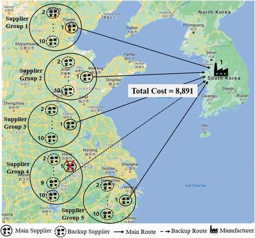
For describing a material flow of the proposed SCN model, we assume the situation that some parts are prepared in China and then sent to a manufacturer in South Korea. The material flow for this situation is shown in Figure 1. As shown in Figure 1, four types of parts are sent to the manufacturer, and each part is prepared at four supplier groups (i.e. supplier group 1 for part 1, supplier group 2 for part 2, supplier group 3 for part 3, and supplier group 4 for part 4). Each supplier group has one main supplier with one main route and two backup suppliers with each one backup route.

Figure 1. Material flows for proposed SCN Model.

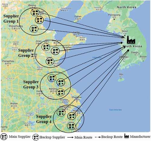
Assuming the situation that 100 parts at each supplier group are sent to the manufacturer, the material flow under considering facility (i.e. main supplier) and route (i.e. main route) disruptions is as follow. The main supplier at supplier group 1 sends part 1 of 100 to the manufacturer using its main route under no disruption risk. However, if the main supplier is completely disrupted with 100% probability, then one of the two backup suppliers sends part 1 of 100 to the manufacturer using its backup route, whereas, if the main supplier is partially disrupted with 50% probability, then it sends 50% of whole amount of part 1 to the manufacturer using its main route and the one of the two backup suppliers send the remainder (50% of whole amount of part 1) to the manufacturer using its backup route.

Also, if the main route of the main supplier is completely disrupted with 100% probability, then one of the two routes (i.e. two backup routes of two backup suppliers) can be used for sending part 1 of 100 to the manufacturer. However, if the main route of the main supplier is partially disrupted with 50% probability, then 50% of whole amount of part 1 are sent to the manufacturer using its main route, and the remainder (50% of whole amount of part 1) are sent to the manufacturer using one of the two routes (i.e. two backup routes of two backup suppliers). The same situations can be also shown in the supplier groups 2, 3 and 4 for parts 2, 3 and 4, respectively.

3. Mathematical formulation

The following assumptions are used for formulating the proposed SCN model.

• A single type product is considered.

• The main supplier and main route at each supplier group are used for sending each part to manufacturer. However, if main supplier in each supplier group is disrupted, then backup suppliers in each supplier group are used. Also, if the main route of main supplier in each supplier group is disrupted, then the backup routes of backup suppliers in each supplier group are used.

• When choosing backup suppliers at each supplier group, any priority does not be considered.

• The number of supplier groups, their suppliers and manufacturers are fixed and already known.

• The operating costs of the main supplier and backup suppliers at each supplier group are different from each other and already known.

• The unit handling costs of main supplier and backup suppliers at each supplier group are different from each other and already known.

• The unit transportation costs between all suppliers at each supplier group and manufacturer are different from each other and already known.

• The proposed SCN model is considered to be in a steady-state situation

• Indices, sets, parameters, and decision variables are defined as follows:¹

• Sets and Indices

$G$ set of supplier groups, indexed by $g$

$S$ set of main suppliers, indexed by $s$

$S^{\prime }$ set of backup suppliers, indexed by $s\prime$

$R$ set of main routes, indexed by $r$

$R^{\prime }$ set of backup routes, indexed by $r\prime$

$M$ set of manufacturers, indexed by $m$

• Parameters

$F_{1gs}$ fixed cost at main supplier s of supplier group g.

$F_{2gs{ }^{\mathrm{\prime }}}$ fixed cost at backup supplier $s{ }^{\mathrm{\prime }}$ of supplier group g.

$H_{1gs}$ unit handling cost at main supplier s of supplier group g.

$H_{2gs{ }^{\mathrm{\prime }}}$ unit handling cost at backup supplier $s{ }^{\mathrm{\prime }}$ of supplier group g.

$T_{1mgsr}$ unit transportation cost from main supplier s of supplier group g to manufacturer m using main route r.

$T_{2mgs{ }^{\mathrm{\prime }}r{ }^{\mathrm{\prime }}}$ unit transportation cost from backup supplier $s{ }^{\mathrm{\prime }}$ of supplier group g to manufacturer m using backup route $r\prime$.

$Q_{1mgsr}$ quantity transported from main supplier s of supplier group g to manufacturer m using main route r.

$Q_{2mgs{ }^{\mathrm{\prime }}r{ }^{\mathrm{\prime }}}$ quantity transported from backup supplier $s{ }^{\mathrm{\prime }}$ of supplier group g to manufacturer m using backup route $r{ }^{\mathrm{\prime }}$.

$A_{1gs}$ quantity handled at main supplier s of supplier group g.

$A_{2gs{ }^{\mathrm{\prime }}}$ quantity handled at backup supplier $s{ }^{\mathrm{\prime }}$ at supplier group g.

$C_m$ capacity of manufacturer $m$ .

$P_{1s}$ disruption probability at main supplier s.

$P_{2r}$ disruption probability at main route r.

• Decision variables

$x_{1gs}$ takes the value 1 if main supplier s at supplier group g is available and 0 otherwise.

$x_{2gs{ }^{\mathrm{\prime }}}$ takes the value 1 if backup supplier $s{ }^{\mathrm{\prime }}$ at supplier group g is available and 0 otherwise.

$y_{1gsr}$ takes the value 1 if main route r of main supplier s at supplier group g is available and 0 otherwise.

$y_{2gs{ }^{\mathrm{\prime }}r{ }^{\mathrm{\prime }}}$ takes the value 1 if backup route $r{ }^{\mathrm{\prime }}$ of backup supplier $s{ }^{\mathrm{\prime }}$ at supplier group g is available and 0 otherwise.

The total cost (TC) using total fixed cost (TF), total handling costs (TH) and total transportation cost (TT) is minimized as the objective function.

(1) $\mathrm{m}\mathrm{i}\mathrm{n}TC=TF+TH+TT$(1)

In Equation (1)(1) $\mathrm{m}\mathrm{i}\mathrm{n}TC=TF+TH+TT$(1) , TF and TH are represented using Equations (2)(2) $\sum _g\sum _s{F}_{1gs}\cdot x_{1gs}+\sum _g\sum _{s{ }^{\mathrm{\prime }}}{F}_{2gs{ }^{\mathrm{\prime }}}\cdot x_{2gs{ }^{\mathrm{\prime }}}$(2) and (3(3) $\sum _g\sum _s{H}_{1gs}\cdot A_{1gs}\cdot x_{1gs}+\sum _g\sum _{s{ }^{\mathrm{\prime }}}{H}_{2gs{ }^{\mathrm{\prime }}}\cdot A_{2gs{ }^{\mathrm{\prime }}}\cdot x_{2gs{ }^{\mathrm{\prime }}}$(3) ), respectively.

(2) $\sum _g\sum _s{F}_{1gs}\cdot x_{1gs}+\sum _g\sum _{s{ }^{\mathrm{\prime }}}{F}_{2gs{ }^{\mathrm{\prime }}}\cdot x_{2gs{ }^{\mathrm{\prime }}}$(2)

(3) $\sum _g\sum _s{H}_{1gs}\cdot A_{1gs}\cdot x_{1gs}+\sum _g\sum _{s{ }^{\mathrm{\prime }}}{H}_{2gs{ }^{\mathrm{\prime }}}\cdot A_{2gs{ }^{\mathrm{\prime }}}\cdot x_{2gs{ }^{\mathrm{\prime }}}$(3)

In Equation (1)(1) $\mathrm{m}\mathrm{i}\mathrm{n}TC=TF+TH+TT$(1) , TT is used when the following each condition is considered in the proposed SCN model: First condition is to consider the situation when main supplier at each supplier group is disrupted. Second one is to consider the situation when the main route of main supplier at each supplier group is disrupted. First and second conditions are represented as Equations (4)(4) $\sum _m\sum _g\sum _s\sum _r{T}_{1mgsr}\cdot Q_{1mgsr}\cdot (1-P_{1s})\cdot x_{1gs}\cdot y_{1gsr}+\sum _m\sum _g\sum _{s{ }^{\mathrm{\prime }}}\sum _{r{ }^{\mathrm{\prime }}}{T}_{2mgs{ }^{\mathrm{\prime }}r{ }^{\mathrm{\prime }}}\cdot Q_{2mgs{ }^{\mathrm{\prime }}r{ }^{\mathrm{\prime }}}\cdot P_{1s}\cdot x_{2gs{ }^{\mathrm{\prime }}}\cdot y_{2gs{ }^{\mathrm{\prime }}r{ }^{\mathrm{\prime }}}$(4) and (5(5) $\sum _m\sum _g\sum _s\sum _r{T}_{1mgsr}\cdot Q_{1mgsr}\cdot (1-P_{2r})\cdot x_{1gs}\cdot y_{1gsr}+\sum _m\sum _g\sum _{s{ }^{\mathrm{\prime }}}\sum _{r{ }^{\mathrm{\prime }}}{T}_{2mgs{ }^{\mathrm{\prime }}r{ }^{\mathrm{\prime }}}\cdot Q_{2mgs{ }^{\mathrm{\prime }}r{ }^{\mathrm{\prime }}}\cdot P_{2r}\cdot x_{2gs{ }^{\mathrm{\prime }}}\cdot y_{2gs{ }^{\mathrm{\prime }}r{ }^{\mathrm{\prime }}}$(5) ), respectively.

(4) $\sum _m\sum _g\sum _s\sum _r{T}_{1mgsr}\cdot Q_{1mgsr}\cdot (1-P_{1s})\cdot x_{1gs}\cdot y_{1gsr}+\sum _m\sum _g\sum _{s{ }^{\mathrm{\prime }}}\sum _{r{ }^{\mathrm{\prime }}}{T}_{2mgs{ }^{\mathrm{\prime }}r{ }^{\mathrm{\prime }}}\cdot Q_{2mgs{ }^{\mathrm{\prime }}r{ }^{\mathrm{\prime }}}\cdot P_{1s}\cdot x_{2gs{ }^{\mathrm{\prime }}}\cdot y_{2gs{ }^{\mathrm{\prime }}r{ }^{\mathrm{\prime }}}$(4)

(5) $\sum _m\sum _g\sum _s\sum _r{T}_{1mgsr}\cdot Q_{1mgsr}\cdot (1-P_{2r})\cdot x_{1gs}\cdot y_{1gsr}+\sum _m\sum _g\sum _{s{ }^{\mathrm{\prime }}}\sum _{r{ }^{\mathrm{\prime }}}{T}_{2mgs{ }^{\mathrm{\prime }}r{ }^{\mathrm{\prime }}}\cdot Q_{2mgs{ }^{\mathrm{\prime }}r{ }^{\mathrm{\prime }}}\cdot P_{2r}\cdot x_{2gs{ }^{\mathrm{\prime }}}\cdot y_{2gs{ }^{\mathrm{\prime }}r{ }^{\mathrm{\prime }}}$(5)

The objective function in Equation (1)(1) $\mathrm{m}\mathrm{i}\mathrm{n}TC=TF+TH+TT$(1) should be optimized under satisfying the following constraints.

subject to

(6) $\sum _s{x}_{1gs}+\sum _{s{ }^{\mathrm{\prime }}}{x}_{2gs{ }^{\mathrm{\prime }}}=1,\hspace{0.17em}\mathrm{\forall }g$(6)

(7) $\sum _s\sum _r{y}_{1gsr}+\sum _s\sum _r{y}_{2gs{ }^{\mathrm{\prime }}r{ }^{\mathrm{\prime }}}=1,\mathrm{\forall }g$(7)

(8) $\sum _g\sum _s\sum _r{Q}_{1mgsr}\cdot x_{1gs}\cdot y_{1gsr}\le \sum _g\sum _s{A}_{1gs}\cdot x_{1gs},\mathrm{\forall }m$(8)

(9) $\sum _g\sum _{s{ }^{\mathrm{\prime }}}\sum _{r{ }^{\mathrm{\prime }}}{Q}_{2mgs{ }^{\mathrm{\prime }}r{ }^{\mathrm{\prime }}}\cdot x_{2gs{ }^{\mathrm{\prime }}}\cdot y_{2gs{ }^{\mathrm{\prime }}r{ }^{\mathrm{\prime }}}\le \sum _g\sum _{s{ }^{\mathrm{\prime }}}{A}_{2gs{ }^{\mathrm{\prime }}}\cdot x_{2gs{ }^{\mathrm{\prime }}},\mathrm{\forall }m$(9)

(10) $\begin{array}{rl}& \sum _g\sum _s\sum _r{Q}_{1mgsr}\cdot x_{1gs}\cdot y_{1gsr}+\\ & \sum _g\sum _{s{ }^{\mathrm{\prime }}}\sum _{r{ }^{\mathrm{\prime }}}{Q}_{2mgs{ }^{\mathrm{\prime }}r{ }^{\mathrm{\prime }}}\cdot x_{2gs{ }^{\mathrm{\prime }}}\cdot y_{2gs{ }^{\mathrm{\prime }}r{ }^{\mathrm{\prime }}}\le C_m,\mathrm{\forall }m\end{array}$(10)

(11) $x_{1gs},x_{2gs{ }^{\mathrm{\prime }}},y_{1gsr},y_{2s{ }^{\mathrm{\prime }}r{ }^{\mathrm{\prime }}}\in \left\{0,1\right\},\mathrm{\forall }g,s,s{ }^{\mathrm{\prime }}r,r{ }^{\mathrm{\prime }}$(11)

In Equation (6)(6) $\sum _s{x}_{1gs}+\sum _{s{ }^{\mathrm{\prime }}}{x}_{2gs{ }^{\mathrm{\prime }}}=1,\hspace{0.17em}\mathrm{\forall }g$(6) , the opening/closing decision of the main supplier and backup suppliers at each supplier group is constrained. Another opening/closing decision at the main route of main supplier and the backup routes of backup suppliers is constrained in Equation (7)(7) $\sum _s\sum _r{y}_{1gsr}+\sum _s\sum _r{y}_{2gs{ }^{\mathrm{\prime }}r{ }^{\mathrm{\prime }}}=1,\mathrm{\forall }g$(7) . Equations (8)(8) $\sum _g\sum _s\sum _r{Q}_{1mgsr}\cdot x_{1gs}\cdot y_{1gsr}\le \sum _g\sum _s{A}_{1gs}\cdot x_{1gs},\mathrm{\forall }m$(8) and (9(9) $\sum _g\sum _{s{ }^{\mathrm{\prime }}}\sum _{r{ }^{\mathrm{\prime }}}{Q}_{2mgs{ }^{\mathrm{\prime }}r{ }^{\mathrm{\prime }}}\cdot x_{2gs{ }^{\mathrm{\prime }}}\cdot y_{2gs{ }^{\mathrm{\prime }}r{ }^{\mathrm{\prime }}}\le \sum _g\sum _{s{ }^{\mathrm{\prime }}}{A}_{2gs{ }^{\mathrm{\prime }}}\cdot x_{2gs{ }^{\mathrm{\prime }}},\mathrm{\forall }m$(9) ) show that the amounts transported from main supplier and backup supplier are restricted in the amount handled at main supplier and backup suppliers. The amount transported from main supplier and backup suppliers to manufacturer is restricted in Equation (10)(10) $\begin{array}{rl}& \sum _g\sum _s\sum _r{Q}_{1mgsr}\cdot x_{1gs}\cdot y_{1gsr}+\\ & \sum _g\sum _{s{ }^{\mathrm{\prime }}}\sum _{r{ }^{\mathrm{\prime }}}{Q}_{2mgs{ }^{\mathrm{\prime }}r{ }^{\mathrm{\prime }}}\cdot x_{2gs{ }^{\mathrm{\prime }}}\cdot y_{2gs{ }^{\mathrm{\prime }}r{ }^{\mathrm{\prime }}}\le C_m,\mathrm{\forall }m\end{array}$(10) . All decision variables used in Equations (1)(1) $\mathrm{m}\mathrm{i}\mathrm{n}TC=TF+TH+TT$(1) to (10) should have 0 or 1 for opening/closing of each supplier and route as shown in Equation (11)(11) $x_{1gs},x_{2gs{ }^{\mathrm{\prime }}},y_{1gsr},y_{2s{ }^{\mathrm{\prime }}r{ }^{\mathrm{\prime }}}\in \left\{0,1\right\},\mathrm{\forall }g,s,s{ }^{\mathrm{\prime }}r,r{ }^{\mathrm{\prime }}$(11) .

The proposed SCN model is one of the nonlinear 0–1 integer programming models and is very difficult to be solved by conventional approaches.

4. GA-VNS approach

To the best of our knowledge, most of complicated network models including the proposed SCN model have been known as NP-complete problems (Gen, Lin, Yun, & Inoue, 2018; Savaskan, Bhattacharya, & Van Wassenhove, 2004; Yun, Chuluunsukh, & Gen, 2020). Most of conventional literatures have shown that metaheuristic approaches such as GA, particle swarm optimization, ant colony optimization, Tabu search, Cuckoo search, etc., have been applied to efficiently solve the complicated network models (Gen & Cheng, 2000; Gen, Cheng, & Lin, 2008; Gen et al., 2018; Savaskan et al., 2004; Yun, Chuluunsukh, & Chen, 2018; Yun et al., 2020). However, many situations exist that most of single metaheuristic approaches do not be well applied (Gen & Cheng, 2000; Yun, 2006; Yun, Chung, & Moon, 2013). To cope with this weakness, various hybrid metaheuristic approaches which combine conventional single metaheuristic approaches have been developed and their efficiency and stability have also been proved (Lin, Gen, & Wang, 2009; Xinyu & Liang, 2016; Zhang, Manier, & Manier, 2012). Therefore, as a hybrid metaheuristic approach, the GA-VNS approach is proposed in this paper. As the GA-VNS approach combines GA approach with VNS approach, both the global search ability using GA approach and the local search ability using VNS approach can be achieved simultaneously.

However, many studies on GA-VNS approach have already been done in various literatures (Castelli & Vanneschi, 2014; Dib, Manier, Moalic, & Caminada, 2017, Dib, Moalic, Manier, & Caminada, 2017; Rostami, Paydar, & Asadi-Gangraj, 2020; Sbai, Krichen, & Limam, 2020; Wang, Luo, Liu, & Yue, 2018; Wen, Xu, & Yang, 2011; Zobolas, Tarantilis, & Ioannou, 2009). Therefore, the characteristics, strong points and weak points of conventional GA-VNS approaches should have been examined and summarized.

4.1 Applying solutions to VNS approach

In most of conventional GA-VNS approaches, VNS approach is applied using the solutions obtained after the implementation of GA approach. However, there exists a difference when using the solutions. Some literatures (Babaie-Kafaki, Ghanbari, & Mahdavi-Amiri, 2016; Wang et al., 2018) used the best one solution, while other literatures (Castelli & Vanneschi, 2014; Dib, Manier, & Caminada, 2015; Dib, Manier, Moalic, & Caminada, 2017; Nourmohammadi, Eskandari, Fathi, & Ng, 2021; Paydar & Saidi-Mehrabad, 2013; Rostami et al., 2020; Türkyilmaz & Bulkan, 2015; Wen et al., 2011; Zhai, Liu, & Yang, 2016; Zobolas et al., 2009) applied either all of the solutions or some of best solutions, after the implementation of GA approach. According to conventional literatures, most of them have focused on using either all of the solutions or some of best solutions rather than using the best one solution. By using either all of the solutions or some of best solutions, VNS approach will be able to explore and exploit wide range regions of search space within various neighborhoods, which can allow GA-VNS approach to find better solutions.

4.2 Using Neighborhood-based operators and local search methods in VNS approach

For neighborhood search, various neighborhood-based operators and conventional local search methods have been used in VNS approach. Some literatures (Babaie-Kafaki et al., 2016; Paydar & Saidi-Mehrabad, 2013; Türkyilmaz & Bulkan, 2015 Wang et al., 2018; Zhai et al., 2016; Zhao, Liu, Zhang, Ma, & Zhang, 2017) used neighborhood-based operators such as swap, insertion, interchange operators, while other literatures (Castelli & Vanneschi, 2014; Wang et al., 2018) applied conventional local search methods such as hill climbing method and teaching-learning-based optimization. However, Wang et al. (2018) suggested that a combinational use of neighborhood-based operators and conventional local search methods is more efficient than the use of neighborhood-based operator alone or conventional local search method alone. Also, among the neighborhood-based operators, swap and insertion operators have been known to be more efficient than the others (Zhao et al., 2017).

4.3 Implementing GA-VNS approach

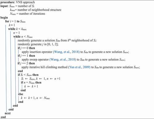
According to the methodologies suggested in sub-sections 4.1 and 4.2, the pGA-VNS approach is proposed here. For the implementation procedure of GA approach, a general procedure such as generating initial population, applying GA operators (i.e. crossover, mutation and selection) is adapted. For the implementation procedure of VNS approach, first, as mentioned in sub-section 4.1, some best solutions taken from offspring at the end of the implementation procedure of GA approach are used for VNS approach. Second, as mentioned in sub-section 4.2, two neighborhood-based operators (i.e. swap and insertion operators) and one local search method (i.e. hill climbing method) are used to find new solution. Last, a solution improvement by comparing conventional solution with new one is achieved.

By combining the implementation procedure of GA approach with that of VNS approach mentioned above, the pGA-VNS approach will be able to explore and exploit the wide range regions of the search space and locate better solutions than conventional GA-VNS approaches. The detailed implementation procedure of the pGA-VNS approach for maximization problem is described in Figures 2 and 3.

Figure 2. Detailed implementation procedure of GA-VNS approach.1997

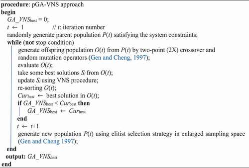
Figure 3. Detailed implementation procedure of VNS approach.

5. Numerical experiments

The SCN models with three different scales are used to compare the performance of the pGA-VNS approach with those of some conventional approaches and to prove the efficiency and stability of the proposed SCN model with disruption risk in this section. The detailed information of supplier groups, suppliers, routes and manufacturers used in the SCN model is shown in Table 2.

Table 2. SCN model with three scales.

Scale	No. of supplier group	No. of Supplier	No. of main supplier	No. of backup supplier	No. of main route	No. of backup route in backup supplier	No. of Manufacturer
1	5	10	1	9	1	9	1
2	10	15	1	14	1	14	1
3	15	30	1	29	1	29	1

The performance of the pGA-VNS approach is compared with two single metaheuristic approaches (i.e. GA by Gen and Chang (2000) and VNS by Mladenović and Hansen (1997)) and two hybrid metaheuristic approaches (i.e. GA-VNS1 by Castelli and Vanneschi (2014) and GA-VNS2 by Sbai et al. (2020)). The difference between the GA-VNS1 and GA-VNS2 approaches is as follows: All solutions of offspring obtained after GA process are applied to the VNS procedure in the GA-VNS1 approach, while, the VNS procedure is used as mutation operator within GA process in the GA-VNS2 approach. Therefore, it will be worthwhile to compare the performances of the GA-VNS1 and GA-VNS2 approaches with that of the pGA-VNS approach, since some solutions of offspring obtained after GA process are applied to the VNS procedure in the pGA-VNS approach.

The conventional approaches (GA, VNS, GA-VNS1, and GA-VNS2) and the pGA-VNS approach were programmed and run under a same computational environment (MATLAB Version 2014b, IBM compatible PC 1.3 GHz processor-Intel core I5-1600 CPU, 4GB RAM, and OS-X EI). The parameter settings for all approaches are as follows: population size is 20, crossover rate 0.4, and mutation rate 0.2 for the search process of GA in the GA, GA-VNS1, GA-VNS2 and pGA-VNS approaches. The number of neighbourhood structure is 5, the number of iterations for each neighborhood structure 5, and the sampling rate extracted from offspring obtained after GA process 10% for the pGA-VNS approach. Above-mentioned all parameter values were used after fine-tuning process. On the other hand, the parameter settings (i.e. the number of neighbourhood structure, the number of iterations for each neighbourhood structure, and the sampling rate extracted from offspring obtained after GA process) for the VNS, GA-VNS1 and GA-VNS2 use the pre-defined values by Mladenović and Hansen (1997), Castelli and Vanneschi (2014), and Sbai et al. (2020), respectively. For all approaches, the total number of iterations is 500. All computation results are obtained after 20 independent runs to eliminate the randomness in the run of each approach. The parameter values to implement the mathematical formulation in Section 3 are defined as shown in Table 3. For various comparison using the performances of all approaches, three measures of performance are used as shown in Table 4.

Table 3. Setting for parameter values.

Parameter	Setting
$F_{gs}$	U [500, 1000]
$F_{gs{ }^{\mathrm{\prime }}}$	U [800, 1200]
$H_{gs}$	U [4, 5]
$H_{gs{ }^{\mathrm{\prime }}}$	U [5, 6]
$T_{mgsr}$	U [1,2]
$T_{mgs{ }^{\mathrm{\prime }}r{ }^{\mathrm{\prime }}}$	U [2, 3]
$Q_{mgsr}$	100
$Q_{mgs{ }^{\mathrm{\prime }}r{ }^{\mathrm{\prime }}}$	100
$A_{gs}$	100
$A_{gs{ }^{\mathrm{\prime }}}$	100
$C_m$	100
$P_s$	U [0.0, 1.0]
$P_r$	U [0.0, 1.0]

Table 4. Three measures for performance comparison.

Measure	Description
Best solution (BS)	Best solution in all trails
Average solution (AS)	Average solution through all trails
Average CPU time (CPU)	Averaged running time through all trails (unit: sec.)

5.1 Scenario-based experiments

To compare the performances of all approaches under various disruption situations of facility and route, three Scenarios (i.e. Scenario 1 to 3) that the main route of main supplier at each supplier group can be disrupted and another three Scenarios (i.e. Scenarios 4 to 6) that main supplier at each supplier group can be disrupted are considered, respectively. The detailed descriptions of each scenario are as follows:

• Scenario 1. The main route of main supplier at one supplier group is disrupted. One of the backup routes of backup suppliers at the supplier group is available.

• Scenario 2. Each main route of main suppliers at two supplier groups are disrupted. One of the backup routes of backup suppliers at each supplier group are available.

• Scenario 3. Each main route of main suppliers at three supplier groups are disrupted. One of the backup routes of backup suppliers at each supplier group are available.

• Scenario 4. The main supplier at one supplier group is disrupted. One of the backup suppliers at the supplier group is available using its backup route.

• Scenario 5. Each main supplier at two supplier groups are disrupted. One of the backup suppliers at each supplier group are available using their backup routes.

• Scenario 6. Each main supplier at three supplier groups are disrupted. One of the backup suppliers at each supplier group are available using their backup routes.

In scenarios 4 to 6, the main suppliers and their main routes are simultaneously disrupted, as the main routes of the main suppliers cannot be also available when the main suppliers are disrupted. The experimental results using all approaches in scenarios 1 to 6 are summarized in Tables 5 to 6.

Table 5. Computation results of each approach in Scenarios 1 to 3.

	GA						VNS					GA-VNS1					GA-VNS2					pGA-VNS
Scenario	Scale	BS	AS	CPU	Gap 1 (%)	Gap	BS	AS	CPU	Gap 1 (%)	Gap 2 (%)	BS	AS	CPU	Gap 1 (%)	Gap	BS	AS	CPU	Gap 1 (%)	Gap 2 (%)	BS	AS	CPU
						2 (%)										2 (%)
1	1	8,974	8,994	1.22	0.93	0.78	8,974	9,255	0.84	0.93	3.71	8,974	8,974	1.45	0.93	0.56	8,974	9,114	2.17	0.93	2.13	8,891	8,924	1.89
	2	15,345	15,368	1.31	0.55	0.22	15,423	15,849	0.86	1.06	3.35	15,345	15,361	1.53	0.55	0.17	15,345	15,449	3.32	0.55	0.74	15,261	15,335	2.35
	3	22,231	22,262	1.82	0	0.03	22,492	22,669	1.56	1.17	1.86	22,231	22,237	1.89	0	−0.09	22,231	22,420	4.71	0	0.74	22,231	22,256	2.67
				Avg.	0.49	0.34			Avg.	1.06	2.97			Avg.	0.49	0.21			Avg.	0.49	1.2
2	1	8,974	9,178	1.22	0.93	1.21	9,395	9,745	0.84	3.61	7.47	8,974	9,199	1.45	0.93	1.44	9,237	9,344	2.17	3.89	3.04	8,891	9,068	1.89
	2	15,548	15,660	1.31	1.32	0.6	15,548	16,087	0.86	−0.12	3.35	15,507	15,622	1.53	1.06	0.36	15,548	15,725	3.32	1.32	1.02	15,345	15,566	2.35
	3	22,424	22,841	1.82	0.21	1.41	22,672	23,126	1.56	0.66	2.67	22,434	22,498	1.89	0.25	−0.12	22,443	22,624	4.71	0.29	0.44	22,378	22,524	2.67
				Avg.	0.82	1.07			Avg.	1.38	4.5			Avg.	0.75	0.56			Avg.	1.83	1.5
3	1	9,207	9,508	1.22	1.68	0.09	9,578	10,166	0.84	5.78	7.02	9,010	9,435	1.45	−0.5	−0.67	9,099	9,390	2.17	0.49	−1.15	9,055	9,499	1.89
	2	15,751	16,050	1.31	1.1	0.87	16,226	16,446	0.86	4.15	3.36	15,607	15,990	1.53	0.17	0.49	15,852	16,061	3.32	1.75	0.94	15,580	15,912	2.35
	3	22,615	22,765	1.82	0.95	0.66	23,137	23,577	1.56	3.28	4.25	22,615	22,838	1.89	0.95	0.98	22,623	22,781	4.71	0.98	0.73	22,403	22,616	2.67
				Avg.	1.24	0.54			Avg.	4.4	4.88			Avg.	0.21	0.27			Avg.	1.07	0.17

Table 6. Computation results of each approach in Scenarios 4 to 6.

	GA						VNS					GA-VNS1						pGA-VNS
Scenario	Scale	BS	AS	CPU	Gap 1 (%)	Gap 2 (%)	BS	AS	CPU	Gap 1 (%)	Gap 2 (%)	BS	AS	CPU	Gap 1 (%)	Gap 2 (%)	BS	AS	CPU	Gap 1 (%)	Gap 2 (%)	BS	AS	CPU
4	1	8,596	9,193	1.220	1.92	0.33	8,935	9,429	0.840	5.94	2.90	8,478	9,166	1.450	0.52	0.03	8,500	9,196	2.170	0.78	0.36	8,434	9,163	1.890
	2	15,365	15,895	1.310	2.40	0.44	15,385	15,920	0.860	2.53	0.59	15,109	16,094	1.530	0.69	1.69	15,154	15,906	3.320	0.99	0.51	15,005	15,826	2.35
	3	22,379	22,711	1.820	7.12	0.67	22,111	22,776	1.560	5.83	0.96	21,800	22,491	1.890	4.35	−0.30	22,258	22,746	4.710	6.54	0.83	20,892	22,559	2.67
				Avg.	3.81	0.48			Avg.	4.77	1.49			Avg.	1.85	0.47			Avg.	2.77	0.56
5	1	8,892	9,309	1.220	3.30	2.75	9,561	9,854	0.840	11.07	8.76	8,931	9,441	1.450	3.75	4.21	8,923	9,412	2.170	3.66	3.89	8,608	9,060	1.890
	2	15,482	16,036	1.310	0.45	0.53	15,554	16,563	0.860	0.92	3.83	15,446	16,072	1.530	0.22	0.75	15,507	16,403	3.320	0.62	2.83	15,412	15,952	2.35
	3	21,981	22,679	1.820	0.88	−0.39	22,389	23,384	1.560	2.75	2.71	21,810	23,000	1.890	0.09	1.02	22,253	23,053	4.710	2.12	1.26	21,790	22,767	2.67
				Avg.	1.54	0.96			Avg.	4.91	5.10			Avg.	1.35	1.99			Avg.	2.13	2.66
6	1	8,831	9,578	1.220	−0.55	0.70	9,814	10,137	0.840	10.52	6.58	9,254	9,492	1.450	4.21	−0.20	9,257	9,507	2.170	4.25	−0.04	8,880	9,511	1.890
	2	15,822	16,521	1.310	2.26	2.77	16,616	16,924	0.860	7.39	5.28	15,832	16,500	1.530	2.33	2.64	15,634	16,162	3.320	1.05	0.54	15,472	16,075	2.35
	3	22,578	23,077	1.820	3.68	1.73	22,838	23,611	1.560	4.88	4.08	22,419	23,042	1.890	2.95	1.57	21,832	22,728	4.710	0.26	0.19	21,776	22,685	2.67
				Avg.	1.80	1.74			Avg.	7.60	5.32			Avg.	3.16	1.34			Avg.	1.85	0.23

* Boldface is the best value at each performance

* Gap 1(%): Difference when compared the performances of GA, VNS, GA-VNS1 and GA-VNS2 with that of pGA-VNS in terms of the BS

* Gap 2(%): Difference when compared the performances of GA, VNS, GA-VNS1 and GA-VNS2 with that of pGA-VNS in terms of the AS

In Tables 5 to 6, the performances of GA, VNS, GA-VNS1 and GA-VNS2 approaches are worse than that of the pGA-VNS approach, if plus (+) values in Gaps 1 and 2 are appeared. However, the former is better than the latter, if minus (-) values in Gaps 1 and 2 are appeared.

In scenario 1 of Table 5, the Gap 1 has the same values of 0.93%, 0.55% and 0.00% in the GA, GA-VNS1 and GA-VNS2 approaches for Scales 1 to 3, which means that the best solutions of the GA, GA-VNS1 and GA-VNS2 approaches are becoming similar to that of the pGA-VNS approach, as the numbers of main suppliers and backup suppliers are increased. However, Gap 2 shows significant differences in the GA, GA-VNS1 and GA-VNS2 approaches, that is, in average solution, the Gap 2 has 0.34%, 0.21%, and 1.20% at each GA, GA-VNS1 and GA-VNS2 approaches, which means that the average solutions of the GA, GA-VNS1 and GA-VNS2 approaches are worse than that of the pGA-VNS approach except Gap 2 of GA-VNS1 approach in Scale 3, regardless of the increase of the numbers of main supplier and backup suppliers.

In the comparison among all conventional approaches, the VNS approach has the worst results in Gaps 1 and 2. In terms of the CPU, the GA, VNS, and GA-VNS1 approaches have similar results each other and slightly quicker than the pGA-VNS approach, whereas, the GA-VNS2 approach is the slowest.

Similar situation is also shown in scenarios 2 and 3. That is, the performances of Gaps 1 and 2 of the GA, GA-VNS1 and GA-VNS2 approaches in average values are similar to each other, while the performances of the VNS approach are the worst. The performances of all conventional approaches (GA, VNS, GA-VNS1 and GA-VNS2) are inferior to the pGA-VNS approach in average values. However, in terms of the CPU, the VNS approach is the quickest and the GA-VNS2 approach is the slowest.

In scenario 4 of Table 6, the GA-VNS1 and GA-VNS2 approaches in Gap 1 of Scales 1 and 2 are similar to each other and have significantly better performances than the GA and VNS approaches. In Gap 1 of Scale 3, the GA approach is the worst. The VNS approach is the worst in Gap 2 of Scales 1 and 3, and the GA-VNS1 approach is the worst in Gap 2 of Scale 2. In average values of Gaps 1 and 2, the VNS approach is significantly inferior to the GA, GA-VNS1 and GA-VNS2 approaches, which is similar to the analysis result of the performances of Gap 2 in Table 5. However, the performances of all conventional approaches (GA, VNS, GA-VNS1 and GA-VNS2) in Gaps 1 and 2 of Scales 1 to 3 are worse than those of the pGA-VNS approach, except the performance of the GA-VNS1 approach in Gap 2 of Scale 3.

Similar situation is also shown in scenarios 5 and 6. That is, the performances of the VNS approach have significantly worse performances when compared with those of the GA, GA-VNS1 and GA-VNS2 approaches in average values of Gaps 1 and 2.

Figures 4 and 5 show the differences of best solutions in Gap 1 and those of average solutions in Gap 2 among all conventional approaches (GA, GA-VNS1 and GA-VNS2) in order to compare their performances more clearly.

Figure 4. Difference of best solutions in Gap 1 among all conventional approaches.

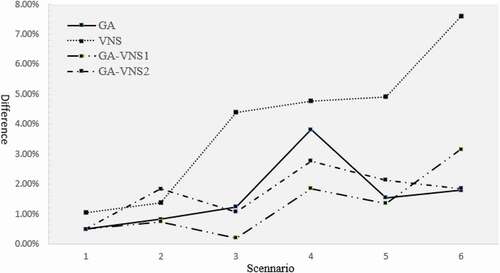
Figure 5. Difference of average solutions in Gap 2 among all conventional approaches.

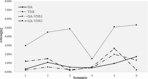
As shown in Figures 4 and 5, the best and average solutions of the VNS approach have higher differences in Scale 1 to 6, and they are significantly worse than those of the GA, GA-VNS1 and GA-VNS2 approach, except that of Scale 2 in Figure 4. The differences shown in Figures 4 and 5 imply that the pGA-VNS approach is more efficient both in best solution and in average solution than all conventional approaches (GA, VNS, GA-VNS1 and GA-VNS2), as all differences in best and average solutions have plus (+) values, which means that the fitness values of all conventional approaches are worse than those of pGA-VNS approach.

For more detailed comparison of all conventional approaches and the pro-HGA approach in their search processes, Figures 6 and 7 show their convergence behaviours as the number of iterations is increased.

Figure 6. Convergence behaviors of each approach in Scale 3 of scenario 3.

Figure 7. Convergence behaviors of each approach in Scale 3 of scenario 6.

In Figure 6, the pGA-VNS approach shows better convergence behaviours than the GA, VNS, GA-VNS1 and GA-VNS2 approaches, though all approaches show various and quick convergence behaviours during initial iterations except the VNS approach. Similar convergence behaviours are also shown in Figure 7. All approaches show various and quick convergence behaviours during initial iterations. However, after approximately 141 iterations, the pGA-VNS approach has a better performance than the others, as all conventional approaches do not show any convergence behaviours.

5.2 Stability and Efficiency in SCN Model

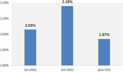
As already analysed in Tables 5 and 6, it is proved that the hybrid metaheuristic approaches (i.e. GA-VNS1 and GA-VNS2) are superior to the single metaheuristic approaches (i.e. GA and VNS) in terms of Gaps 1 and 2. Therefore, it will be worthwhile to compare the performance among the hybrid metaheuristic approaches including the pGA-VNS approach more precisely. Figure 8 shows the average gap in terms of the BS among all scenarios and Scales. As shown in Figure 8, the pGA-VNS approach has 1.97%, while the GA-VNS1 and GA-VNS2 approaches have 2.03% and 2.18%, respectively. The average gap of the pGA-VNS approach is smaller than those of the GA-VNS1 and GA-VNS2 approaches, which means that the fluctuations of the total cost when the pGA-VNS approach is applied to the SCN model are less than those of the total cost when the GA-VNS1 and GA-VNS2 approaches are applied to the SCN model. By this analysis result, we can know that even though more disruption risks in facility and route of the SCN model are occurred, managing and operating the SCN model by the pGA-VNS approach are more stable and efficient than those by the GA-VNS1 and GA-VNS2 approaches.

Figure 8. Average gap in BS values among all scenarios and scales.

Figure 9 shows the opening and closing decision among all suppliers in each supplier group and manufacturer when the pGA-VNS approach is applied to Scale 1. In supplier group 1, it is shown that the main supplier (i.e. No. 1) is opened and all backup suppliers (i.e. Nos. 2 to 10) are closed. Therefore, the opened main supplier sends part 1 to the opened manufacturer (i.e. No. 1) using its main route. Same situations are also shown in supplier groups 2, 3, and 5 for part 2, 3 and 5, respectively. However, in supplier group 4, the backup supplier (i.e. No. 9) is opened and the others (i.e. Nos. 2 to 8 and 10), including main supplier (i.e. No. 1) are closed. Therefore, the opened backup supplier (i.e. No. 9) sends part 4 to the opened manufacturer (i.e. No. 1) using its backup route. By using this SCN model, the total cost shown in Equation (1)(1) $\mathrm{m}\mathrm{i}\mathrm{n}TC=TF+TH+TT$(1) is 8,891 and this value coincides with the BS value of the pGA-VNS approach in Scale 1 of Scenario 1 shown in Table 5.

Figure 9. Opening/closing decision between suppliers and manufacturer in Scale 1.

Based on the results of Tables 5 and 6, and Figures 4 to 8, we can reach the following conclusions.

• The pGA-VNS approach outperforms all the conventional approaches (GA, VNS, GA-VNS1 and GA-VNS2) in best solution and average solution, which implies that the search scheme used in the pGA-VNS approach is more efficient than those in the GA, VNS, GA-VNS1 and GA-VNS2 approaches. However, in average CPU time, the VNS approach is considerably quicker than the pGA-VNS approach, which can be interpreted that the former has the search scheme of VNS only, while the latter has a hybrid search scheme using GA and VNS.

• In the comparison among all conventional approaches (GA, VNS, GA-VNS1, and GA-VNS2), the performances of two hybrid metaheuristic approaches (GA-VNS1 and GA-VNS2) do not show any merits in the average values of Gaps 1 and 2 when compared with that of single metaheuristic approaches (GA), which implies that the VNS search schemes used in the GA-VNS1 and GA-VNS2 approaches are not efficient in searching optimal solution.

• In the comparison among all hybrid meta-heuristics approaches (GA-VNS1, GA-VNS2, and pGA-VNS), the pGA-VNS approach shows better performances in best solution and average solutions than the GA-VNS1 and GA-VNS2 approaches, though some results of the GA-VNS1 and GA-VNS2 approaches in Gaps 1 and 2 are slightly better than those of the pGA-VNS approach. Therefore, in the view of whole computation results of Gaps 1 and 2, it can be shown that the pGA-VNS approach is more efficient than the GA-VNS1 and GA-VNS2 approaches.

6. Conclusion

In the SCN model considering disruption risk, most of conventional studies have focused either on facility disruption solely or on route disruption solely. However, in real-world case, there exist many situations that the disruptions of facility and route can be occurred simultaneously. In this paper, we have proposed a SCN model with the simultaneous consideration of facility and route disruptions. For efficiently representing the proposed SCN model, two kinds of supplier (main supplier and backup supplier) and two kinds of route (main route of main supplier and backup route of backup supplier) have been used in each supplier group.

The proposed SCN model has been formulated as a nonlinear 0–1 integer programming model, and the pGA-VNS approach, one of hybrid metaheuristic approaches, has been used for implementing the proposed SCN model. In numerical experiments, the proposed SCN models with three scales have been presented and the performance of the pGA-VNS approach have been compared with those of two single metaheuristic approaches (GA and VNS) and two hybrid metaheuristic approaches (GA-VNS1 and GA-VNS2) using some measure of performances.

For more various comparisons among the GA, VNS, GA-VNS1, GA-VNS2, and pGA-VNS approaches, experiments have been divided into two sub sections.

In sub-section 5.1, scenario-based experimental comparisons have been made. Six scenarios considering various disruption situations of facility and route have been used. The experimental results have shown that the pGA-VNS approach outperforms all conventional approaches (GA, VNS, GA-VNS1 and GA-VNS2) in best and average solutions, except average CPU time. In the comparison among the convergence behaviours of each approach, the pGA-VNS approach has shown to be more various and quick convergence behaviours than the other competing approaches.

In sub-section 5.2, the stability and efficiency of the SCN model have been reviewed for more precise comparison among the GA-VNS1, GA-VNS2, and pGA-VNS approaches. By using average gap in the BS value among all scenarios and scales, it can be observed that managing and operating the SCN model by the pGA-VNS approach are more stable and efficient than those by the GA-VNS1 and GA-VNS2 approaches, though more disruption risks in facility and route of the SCN model are occurred.

By various analyses using sub-sections 5.1 and 5.2, we can confirm that the stability and efficiency of the proposed SCN model can be reinforced. However, since the proposed SCN model has a simple supply chain structure using several suppliers and manufacturers, it will be extended as a multi-stage SCN model linked with various suppliers, manufacturers, distribution centers, retailers and customers. An effort for reducing the search speed of the pGA-VNS approach should be also required, though it has significantly better performances in best and average solutions than the other competing approaches. These two weaknesses of the proposed SCN model and pGA-VNS approach will be left to our future research direction.

Acknowledgments

This study was supported by research fund from Chosun University, 2021

Disclosure statement

No potential conflict of interest was reported by the author(s).

Additional information

Funding

This work was supported by the Chosun University [2021].

Notes

1. please change it . Indices, sets, parameters, and decision variables are defined as follows: ==> Indices, sets, parameters, and decision variables are defined as follows:

References

- Arabsheybani, A., & Khasmeh, A. A. (2021). Robust and resilient supply chain network design considering risks in food industry: Flavour industry in Iran. International Journal of Management Science and Engineering Management, 16(3), 197–208.
- Azaron, A., Venkatadri, U., & Doost, A. F. (2021). Designing profitable and responsive supply chains under uncertainty. International Journal of Production Research, 59(1), 213–225.
- Babaie-Kafaki, S., Ghanbari, R., & Mahdavi-Amiri, N. (2016). Hybridizations of genetic algorithms and neighborhood search metaheuristics for fuzzy bus terminal location problems. Applied Soft Computing, 46, 220–229.
- Baghalian, A., Rezapour, S., & Farahani, R. Z. (2013). Robust supply chain network design with service level against disruptions and demand uncertainties: A real-life case. European Journal of Operational Research, 227(1), 199–215.
- Baz, J. E., & Ruel, S. (2021). Can supply chain risk management practices mitigate the disruption impacts on supply chains’ resilience and robustness? Evidence from an empirical survey in a COVID-19 outbreak era. International Journal of Production Economics, 233, 107972.
- Castelli, M., & Vanneschi, L. (2014). Genetic algorithm with variable neighborhood search for the optimal allocation of goods in shop shelves. Operations Research Letters, 42(5), 355–360.
- Chopra, S., & Sodhi, M. S. (2004). Managing risk to avoid supply chain breakdown. MIT Sloan Management Review, 46(1), 53–62.
- Dib, O., Manier, M.-A., & Caminada, A. (2015). Memetic algorithm for computing shortest paths in multimodal transportation networks. Transportation Research Procedia, 10, 745–755.
- Dib, O., Manier, M.-A., Moalic, L., & Caminada, A. (2017). Combining VNS with genetic algorithm to solve the one-to-one routing issue in road networks. Computers & Operations Research, 78, 420–430.
- Dib, O., Moalic, L., Manier, M.-A., & Caminada, A. (2017). An advanced GA–VNS combination for multicriteria route planning in public transit networks. Expert Systems with Applications, 72, 67–82.
- Dolgui, A., & Ivanov, D. (2021). Ripple effect and supply chain disruption management: New trends and research directions. International Journal of Production Research, 59(1), 102–109.
- DuHadway, S., Carnovale, S., & Hazen, B. (2019). Understanding risk management for intentional supply chain disruptions: Risk detection, risk mitigation, and risk recovery. Annals of Operations Research, 283(1–2), 179–198.
- Gedik, R., Medal, H., Rainwater, C., Pohl, E. A., & Mason, S. J. (2014). Vulnerability assessment and re-routing of freight trains under disruptions: A coal supply chain network application. Transportation Research Part E, 71, 45–57.
- Gen, M., & Cheng, R. (1997). Genetic algorithms and engineering design. New York, NY, USA: John-Wiley & Sons.
- Gen, M., & Cheng, R. (2000). Genetic algorithms and engineering optimization. New York, NY, USA: John-Wiley & Sons.
- Gen, M., Cheng, R., & Lin, L. (2008). Network models and optimization: Multiple objective genetic algorithm approach. London, UK: Springer.
- Gen, M., Lin, L., Yun, Y. S., & Inoue, H. (2018). Recent advances in hybrid priority-based genetic algorithms for logistics and SCM network design. Computers & Industrial Engineering, 125, 394–412.
- Jabbarzadeh, A., Haughton, M., & Khosrojerdi, A. (2018). Closed-loop supply chain network design under disruption risks: A robust approach with real world application. Computers & Industrial Engineering, 116, 178–191.
- Lin, L., Gen, M., & Wang, X. (2009). Integrated multistage logistics network design by using hybrid evolutionary algorithm. Computers & Industrial Engineering, 5(6), 854–873.
- Martha, J., & Subbakrishna, S. (2002). Targeting a just-in-case supply chain for the inevitable next disaster. Supply Chain Management Review, 6(5), 18–23.
- Mladenović, N., & Hansen, P. (1997). Variable neighborhood search. Computers and Operations Research 24(11), 1097–1100.
- Monahan, S., Laudicina, P., & Attis, D. (2003). Supply chains in a vulnerable volatile world. Executive Agenda, 6(3), 5–15.
- Nourmohammadi, A., Eskandari, H., Fathi, M., & Ng, A. H. C. (2021). Integrated locating in-house logistics areas and transport vehicles selection problem in assembly lines. International Journal of Production Research, 59(2), 598–616.
- Paydar, M. M., & Saidi-Mehrabad, M. (2013). A hybrid genetic-variable neighborhood search algorithm for the cell formation problem based on grouping efficacy. Computers & Operations Research, 40, 980–990.
- Poudel, S. R., Marufuzzaman, M., & Bian, L. (2016). Designing a reliable bio-fuel supply chain network considering link failure probabilities. Computers & Industrial Engineering, 91, 85–99.
- Rahman, M. H., Rifat, M., Azeem, A., & Ali, S. M. (2018). A quantitative model for disruptions mitigation in a supply chain considering random capacities and disruptions at supplier and retailer. International Journal of Management Science and Engineering Management, 13(4), 265–273.
- Ramshani, M., Ostrowski, J., Zhang, K., & Li, X. (2019). Two level uncapacitated facility location problem with disruptions, Computers and. Industrial Engineering, 137, 106089.
- Rostami, A., Paydar, M. M., & Asadi-Gangraj, E. (2020). A hybrid genetic algorithm for integrating virtual cellular manufacturing with supply chain management considering new product development. Computers and Industrial Engineering, 145, 106565.
- Savaskan, R. C., Bhattacharya, S., & Van Wassenhove, L. V. (2004). Closed-loop supply chain models with product manufacturing. Management Science, 50(2), 239–252.
- Sbai, I., Krichen, S., & Limam, O. (2020). Two meta-heuristics for solving the capacitated vehicle routing problem: The case of the Tunisian post office. Operational Research, 20, 2085–2108.
- Tang, C. S. (2006). Perspectives in supply chain risk management. International Journal of Production Economics, 103(2), 451–488.
- Trkman, P., & McCormack, K. (2009). Supply chain risk in turbulent environments—A conceptual model for managing supply chain network risk. International Journal of Production Economics, 119(2), 247–258.
- Türkyilmaz, A., & Bulkan, S. (2015). A hybrid algorithm for total tardiness minimisation in flexible job shop: Genetic algorithm with parallel VNS execution. International Journal of Production Research, 53(6), 1748–1832.
- Wang, K., Luo, H., Liu, F., & Yue, X. (2018). Permutation flow shop scheduling with batch delivery to multiple customers in supply chains. IEEE Transactions on Systems, Man, and Cybernetics: Systems, 48(10), 1826–1837.
- Wang, X., Ruan, J., & Shi, Y. (2012). A recovery model for combinational disruptions in logistics delivery: Considering the real-world participators. International Journal of Production Economics, 140(1), 508–520.
- Waters, D. (2007). Supply chain risk management: Vulnerability and resilience in logistics. London, UK: Kogan Page limited.
- Wen, Y., Xu, H., & Yang, J. (2011). A heuristic-based hybrid genetic-variable neighborhood search algorithm for task scheduling in heterogeneous multiprocessor system. Information Sciences, 181(3), 567–581.
- Wilson, M. C. (2007). The impact of transportation disruptions on supply chain performance. Transportation Research Part E, 43, 295–320.
- Xiao, T., & Yu, G. (2006). Supply chain disruption management and evolutionarily stable strategies of retailers in the quantity-setting duopoly situation with homogeneous goods. European Journal of Operational Research, 173(2), 648–668.
- Xinyu, L., & Liang, G. (2016). An effective hybrid genetic algorithm and Tabu search for flexible job shop scheduling problem. International Journal of Production Economics, 174, 93–110.
- Yun, Y. S. (2006). Hybrid genetic algorithm with adaptive local search scheme. Computers and Industrial Engineering, 51, 128–141.
- Yun, Y. S., Chuluunsukh, A., & Chen, X. (2018). Hybrid genetic algorithm for optimizing closed-loop supply chain model with direct shipment and delivery. New Physics: Sae Mulli, 68(6), 683–692.
- Yun, Y. S., Chuluunsukh, A., & Gen, M. (2020). Sustainable closed-loop supply chain design problem: A hybrid genetic algorithm approach. Mathematics, 8(1), 84.
- Yun, Y. S., Chung, H. S., & Moon, C. U. (2013). Hybrid genetic algorithm approach for precedence-constrained sequencing problem. Computers & Industrial Engineering, 65(1), 137–147.
- Zhai, H., Liu, Y.-K., & Yang, K. (2016). Modeling two-stage UHL problem with uncertain demands. Applied Mathematical Modelling, 40(4), 2048–3029.
- Zhang, Q., Manier, H., & Manier, M. A. (2012). A genetic algorithm with Tabu search procedure for flexible job shop scheduling with transportation constraints and bounded processing times. Computers & Operations Research, 39(7), 1713–1723.
- Zhao, F., Liu, Y., Zhang, Y., Ma, W., & Zhang, C. A. (2017). Hybrid harmony search algorithm with efficient job sequence scheme and variable neighborhood search for the permutation flow shop scheduling problems. Engineering Applications of Artificial Intelligence, 65, 178–199.
- Zobolas, G. I., Tarantilis, C. D., & Ioannou, G. (2009). Minimizing makespan in permutation flow shop scheduling problems using a hybrid metaheuristic algorithm. Computers & Operations Research, 36(4), 1249–12670.