Abstract
We consider a three-stage discrete-time population model with density-dependent survivorship and time-dependent reproduction. We provide stability analysis for two types of birth mechanisms: continuous and seasonal. We show that when birth is continuous there exists a unique globally stable interior equilibrium provided that the inherent net reproductive number is greater than unity. If it is less than unity, then extinction is the population's fate. We then analyze the case when birth is a function of period two and show that the unique two-cycle is globally attracting when the inherent net reproductive number is greater than unity, while if it is less than unity the population goes to extinction. The two birth types are then compared. It is shown that for low birth rates the adult average number over a one-year period is always higher when reproduction is continuous. Numerical simulations suggest that this remains true for high birth rates. Thus periodic birth rates of period two are deleterious for the three-stage population model. This is different from the results obtained for a two-stage model discussed by Ackleh and Jang (J. Diff. Equ. Appl., 13, 261–274, 2007), where it was shown that for low birth rates seasonal breeding results in higher adult averages.
1. Introduction
Several researchers have focused in recent years on the dynamics of nonautonomous discrete-time models and the advantage of seasonal versus continuous breeding in terms of maximizing the total population number or the total number of adults over a fixed time period Citation1–10. These studies were motivated by an experimental system which investigated the responses of populations of the flour beetle, Tribolium castaneum, cultured in a series of regularly fluctuating environments. Therein, it was observed that population density declined as environmental period lengthened Citation11.
Motivated by an urban population of green treefrogs that we are studying Citation12, we recently developed the following juvenile–adult model for a seasonally breeding population Citation13:
In that paper we focused on the following question: given that an adult recruits a fixed number of juveniles in one year, is it advantageous (in terms of maximizing the total number of adults over a period of one year) to reproduce continuously or seasonally? To answer this question, we investigated the model dynamics for two types of recruitment: continuous (i.e. b
t
= b > 0 for t = 0, 1, 2, …) and periodic with period two (i.e. , b
1 = 0,
).
Our analysis showed that for low birth rates, the population which produces seasonally may survive while the one which reproduces continuously will go to extinction. Thus seasonal breeding is beneficial for such values of birth rates. Furthermore, we show that for low values of birth rates where both populations persist, the adults for the continuously breeding population have a lower average over a one-year period than the one that produces seasonally. Therefore, seasonal reproduction is beneficial in this case. However, for high birth rates this conclusion reverses, and it is shown that breeding continuously results in higher adult averages over a one-year period.
The purpose of this paper is to continue this investigation for a three-stage discrete time model. In section 2 we present the model and analyze the continuous breeding case, and show that if the inherent net reproductive number is less than unity then the population goes to extinction, while if it is greater than unity then the unique interior equilibrium is globally asymptotically stable. We then analyze the seasonal breeding with period-two and show that if the inherent net reproductive number is less than unity then the population becomes extinct, while if it is greater than unity the unique two-cycle is globally attracting. At the end of this section we compare the two birth types and show that in this case (unlike the two-stage model) breeding seasonally seems always to be deleterious. In section 3 we provide concluding remarks.
2. Model development and analysis
We develop a theoretical model describing the dynamics of a population which engages in seasonal breeding and is divided into three stages: a juvenile stage, nonbreeding (sexually immature) stage, and breeding (adult) stage. To this end, denote by x t the number of juveniles at time t, by y t the number of nonbreeding individuals at time t and by z t the number of adults at time t. We assume that the juvenile and nonbreeding stages are less than or equal to one time unit (i.e. all juveniles and nonbreeders move into the next stage within one time step). Assume that competition occurs within each stage. We then obtain the following nonautonomous three-stage discrete model:
-
(H1)
, s i (0) = a i , 0 < a i < 1,
Theorem 2.1
Let x*∈I be an equilibrium of
Equation(2). Suppose F satisfies the following two conditions:
-
(a) F is non-decreasing in each of its arguments, and
-
(b) F satisfies
2.1 Continuous breeding
In this subsection we consider model Equation(1) with continuous breeding. In particular, we assume that in model Equation(1)
b
t
≡ b, a positive constant. Clearly solutions of system Equation(1)
remain positive. The system always has a trivial steady state E
0 = (0, 0, 0). The z-component of a nontrivial steady state
, must satisfy
Theorem 2.2
If R
0 < 1, then (1) has only the trivial steady state E
0 = (0, 0, 0) which is globally asymptotically stable. If R
0 > 1, then E
0
is unstable and (1) has another equilibrium
which is globally asymptotically stable in the interior of
.
Proof
Suppose R
0 < 1. Let be a solution of Equation(1)
. Since
and
for t ≥ 0, consider the following linear system
Suppose now R
0 > 1. It is clear that E
0 is unstable by the above analysis. We first verify that E
1 is locally asymptotically stable. The linearization of Equation(1) with respect to E
1 yields the following Jacobian matrix J(E
1):
Observe that J
21 > 0, J
32 > 0, and J
33 > 0 by our assumptions of (H1). Since satisfies Equation(3)
,
, and
, we have by Equation(3)
that
To show that E
1 is globally attracting in the interior of , we apply Theorem 2.1. Notice system Equation(1)
can be converted into the following third-order scalar difference equation:
2.2 Seasonal breeding
In this subsection we assume that breeding is seasonal where the function b
t
in Equation(1) is periodic with period two. Specifically, we set
. Let
be given. It is clear that
for t > 0. Moreover, x
1 = 0,
,
,
, y
2 = 0 and
. Therefore, if (x
0, y
0, z
0) is a part of a two-cycle, then we have x
2 = x
0, y
2 = y
0 = 0 and
. As a result, if z
0≠0, then z
0 must satisfy
Theorem 2.3
If
, then E
0 = (0, 0, 0) is globally asymptotically stable for (1).
Proof
We first show that E 0 is globally attracting by using a simple comparison method. Observe that x 2t + 1 = 0 for t ≥ 0 and y 2t = 0 for t ≥ 1. Also
Since system Equation(1) is periodic with period two, the local stability of E
0 depends on the product of the matrices Citation16:
Suppose now . Then it follows from the proof of Theorem 2.3 that E
0 is unstable. Moreover, Equation(1)
has a unique two-cycle:
Theorem 2.4
If
, then the two-cycle is globally asymptotically stable for system
Equation(1)
in the interior of
.
Proof
We first prove that the two-cycle is locally asymptotically stable. Recall that its stability depends on the eigenvalues of the product of the matrices Citation16:
It remains to show that the two-cycle is globally attracting in the interior of . The proof is similar to the proof of Theorem 2.2. Let
be given. Observe that x
2t + 1 = 0 for t ≥ 0 and y
2t
= 0 for t ≥ 1. It follows that for t ≥ 1
2.3 Comparison between continuous and seasonal breeding
For the rest of this section we assume that in a continuous or seasonal breeding population an adult reproduces the same number of juveniles in a one-year period. Thus, we let . We are interested to see for what values of b continuous breeding (seasonal breeding) is advantageous in terms of maximizing the average number of adults over a one-year period.
(a) Persistence of population with continuous reproduction
Since , then Theorem 2.2 and Theorem 2.4 require, respectively, that
(b) Comparison of the breeding adults for periodic and constant birth rates
Differ-entiate both sides of equilibrium Equationequation (3) with respect to b yields
, where
We provide numerical results verifying our theoretical conclusions. In , we choose a set of parameters that results in the continuous birth population converging to a positive equilibrium while the population with period-two birth rate goes to extinction. In this case, while
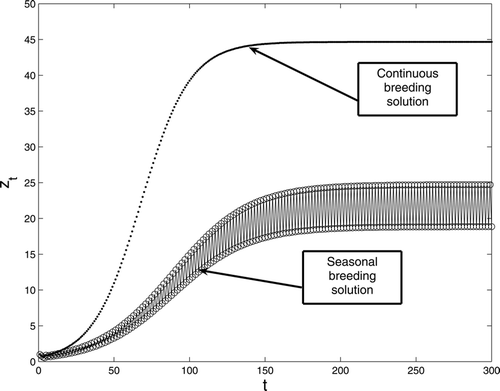
. Increasing the birth rate, we present the results in . In this case, R
0 = 1.5 > 1 while
. Thus, both populations survive. One converges to a positive equilibrium and the other converges to a positive two-cycle. Clearly, the equilibrium value for adults z
t
is larger than the average two-cycle. Thus continuous reproduction is advantageous for this birth rate value.
Figure 1. A comparison between continuous and seasonal breeding with period two birth rate for model Equation(1). The survivorship functions are s
1(x) = a
1/(1 + k
1
x), s
2(y) = a
2/(1 + k
2
y), s
3(z) = a
3/(1 + k
3
z) with parameter values a
1 = 0.3, a
2 = 0.5, a
3 = 0.8, k
1 = 0.001, k
2 = 0.0015, k
3 = 0.002 and b = 1.35 and
. The initial conditions are given by x
0 = 0, y
0 = 0, and z
0 = 1.
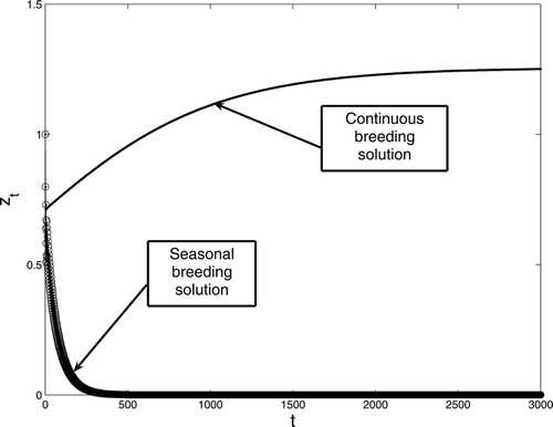
Figure 2. A comparison between continuous and seasonal breeding with period two birth rate for model Equation(1). The survivorship functions are s
1(x) = a
1/(1 + k
1
x), s
2(y) = a
2/(1 + k
2
y), s
3(z) = a
3/(1 + k
3
z) with parameter values a
1 = 0.3, a
2 = 0.5, a
3 = 0.8, k
1 = 0.001, k
2 = 0.0015, k
3 = 0.002 and b = 2 and
. The initial conditions are given by x
0 = 0, y
0 = 0, and z
0 = 1.
3. Concluding remarks
In this paper we have shown that for the three-stage discrete-time population model Equation(1) a periodic birth rate with period two is deleterious for low birth rates, as it will result in smaller average of adults in comparison with a continuous birth rate even though in both cases each adult reproduces the same number of juveniles per year. Numerical simulations of model Equation(1)
suggest that this conclusion remains true for large birth rates. This is in contrast with the result for a two-stage discrete model, which shows that when birth rates are low, seasonal reproduction is advantageous, while when birth rates are high continuous breeding is advantageous. The reason for this is that for a juvenile to become a breeding adult it has to survive two time units (two stages). Thus, a period two birth rate is not enough to compensate for this. Therefore, the seasonally breeding population needs to concentrate its breeding over a shorter time period. However, this period cannot be too short. If, for example, the seasonal population resorts to a period three birth rate, then numerical simulations of model Equation(1)
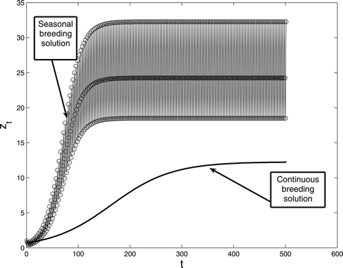
suggest that the conclusion is similar to that of the two-stage model with period two birth rate Citation13. That is, for low birth rates the three-stage model with period three birth rate results in higher adult averages than the continuous breeding population (see for an example).
Figure 3. A comparison between continuous and seasonal breeding with period three birth rate for model Equation(1). The survivorship functions are s
1(x) = a
1/(1 + k
1
x), s
2(y) = a
2/(1 + k
2
y), s
3(z) = a
3/(1 + k
3
z) with parameter values a
1 = 0.3, a
2 = 0.5, a
3 = 0.8, k
1 = 0.001, k
2 = 0.0015, k
3 = 0.002 and b = 1.5 and
. The initial conditions are given by x
0 = 0, y
0 = 0 and z
0 = 1.
Similarly, if the birth rate has period four, then seasonal breeding results in higher adult averages for low birth rates. However, if the birth rate has period-five, then our numerical simulations suggest that seasonal breeding is always deleterious. Thus, the conclusion is similar to a period two birth rate.
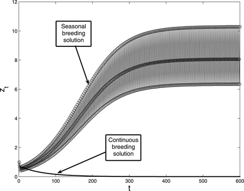
If the population with three stages have a seasonal breeding of period three, i.e. b
0 = 0, b
1 = 0, , b
3 = 0, b
4 = 0 and
then one can show that by defining
the inherent net reproductive number for this population, a unique three-cycle exists provided that
. We conjecture that this three-cycle is globally attracting provided that
. While if
then the population becomes extinct. These results should follow by using a similar argument as in section 2 (which involves lengthy computations). Thus, if
(i.e. each individual reproduces in one season the same number of juveniles as an individual who reproduces continuously breeds in an entire year) then both populations persist if:
Figure 4. A comparison between continuous and seasonal breeding with period three birth rate for model Equation(1). The survivorship functions are s
1(x) = a
1/(1 + k
1
x), s
2(y) = a
2/(1 + k
2
y), s
3(z) = a
3/(1 + k
3
z) with parameter values a
1 = 0.3, a
2 = 0.5, a
3 = 0.8, k
1 = 0.001, k
2 = 0.0015, k
3 = 0.002 and b = 1.2 and
. The initial conditions are given by x
0 = 0, y
0 = 0 and z
0 = 1.
Acknowledgements
The work of A.S. Ackleh is partially supported by the National Science Foundation under grant # DUE-0531915.
References
- Costantino , R. F. , Cushing , J. M. , Dennis , B. , Desharnai , A. and Henson , S. M. 1998 . Resonant population cycles in temporally fluctuating habitats . Bulletin of Mathematical Biology , 60 : 247 – 275 .
- Cushing , J. M. and Henson , S. M. 2001 . Global dynamics of some periodically forced monotone difference equations . Journal of Difference Equations and Applications , 7 : 850 – 872 .
- Cushing , J. M. and Henson , S. M. 2002 . A periodically forced Beverton–Holt equation . Journal of Difference Equations and Applications , 8 : 1119 – 1120 .
- Cushing , J. M. 2006 . A juvenile–adult model with periodic vital rates . Journal of Mathematical Biology , 53 : 520 – 539 .
- Elaydi , S. and Sacker , R. J. 2005 . Nonautonomous Beverton–Holt equations and the Cushing–Henson conjectures . Journal of Difference Equations and Applications , 11 : 337 – 346 .
- Elaydi , S. and Sacker , R. J. 2005 . Global stability of periodic orbits of non-autonomous difference equations and population biology . Journal of Difference Equations , 208 : 258 – 273 .
- Franke , J. E. and Yakubu , A. 2005 . Population models with periodic recruitment functions and survival rates . Journal of Difference Equations and Applications , 11 : 1169 – 1184 .
- Henson , S. M. and Cushing , J. M. 1997 . The effects of periodic habitat fluctuations on a nonlinear insect population model . Journal of Mathematical Biology , 36 : 201 – 226 .
- Henson , S. M. , Costantino , R. F. , Cushing , J. M. , Dennis , B. and Desharnais , R. 1999 . Multiple attractors, saddles, and population dynamics in periodic habitats . Bulletin of Mathematical Biology , 61 : 1121 – 1149 .
- Kocic , V. L. 2005 . A note on the nonautonomous Beverton–Holt model . Journal of Difference Equations and Applications , 11 : 415 – 422 .
- Jillson , D. 1990 . Insect populations respond to fluctuating environments . Nature , 288 : 699 – 700 .
- Pham , L. , Boudreaux , S. , Karhbet , S. , Price , B. , Ackleh , A. S. , Carter , J. and Pal , N. Population estimates of Hyla cinerea (Schneider) in an urban environment . Southeastern Naturalist , 6 203 – 216 .
- Ackleh , A. S. and Jang , S. 2007 . A discrete two-stage population model: continuous versus seasonal reproduction . Journal of Difference Equations and Applications , 13 : 261 – 274 .
- Grove , A. and Ladas , G. 2005 . Periodicities in Nonlinear Difference Equations , Boca Raton : CRC Press .
- Allen , L. J.S. 2007 . Introduction to Mathematical Biology , Englewood Cliffs, NJ : Prentice Hall .
- Caswell , H. 2001 . Matrix Population Models: Construction, Analysis, and Interpretation , Second Edition , Sunderland, MA : Sinauer .