Rabies in raccoons: optimal control for a discrete time model on a spatial grid

Abstract

An epidemic model for rabies in raccoons is formulated with discrete time and spatial features. The goal is to analyze the strategies for optimal distribution of vaccine baits to minimize the spread of the disease and the cost of implementing the control. Discrete optimal control techniques are used to derive the optimality system, which is then solved numerically to illustrate various scenarios.

Keywords:

• Rabies in raccoons
• Discrete model
• Optimal control
• Vaccine

1. Introduction

Several distinct rabies virus variants have been identified in wildlife in the United States, with raccoons the most frequently reported rabid species. Raccoons are the primary vector for rabies in the eastern United States 1. Currently, 15 states distribute oral rabies vaccine for raccoons. The vaccine is encased with a plastic package coated in fish meal and oil. When the raccoon eats the bait, there is an immune response to the rabies antigen which creates antibodies to fight off the disease 2. We present methods here that consider the analysis of spatial and temporal patterns for distributing vaccine baits. Our objective is to investigate the effects of alternative bait distribution patterns on the spread of rabies among raccoons.

Rabies models have mostly used ordinary differential equations (ODEs) and partial differential equations (PDEs). The papers by Murray and collaborators 3, 4 studied the spatial spread of rabies among foxes in England using PDEs. Using the model from 4, Evans and Pritchard 5 applied control of initial conditions in culling and quarantine to drive the population to a desired profile. Coyne, Smith, and McAllister formulated an ODE system for rabies in raccoons 6, which makes explicit the development of natural immunity to rabies and used this to evaluate culling and vaccination strategies. In this model, six classes were considered: susceptible raccoons, infected but noninfectious raccoons that develop rabies, infected but noninfectious raccoons that eventually develop immunity, rabid raccoons, raccoons that are immune as a result of natural infection, and vaccinated raccoons. Both discrete deterministic and stochastic models were analyzed by Allen, Flores, Ratnayake and Herbold 7. Their models are structured with respect to space (m patches), age (juvenile and adults) and three disease states: susceptible, infected and vaccinated. An SEIR (susceptible, exposed, infectious, and recovered) model was developed to describe the spatial and temporal patterns of a raccoon rabies epizootic in 8 by applying an ODE system at different spatial locations.

In a series of papers, Real and collaborators 9–11 developed a stochastic discrete-event simulator for the spread of raccoon rabies for which the infection of geographic locations (e.g. townships) occurred at a unique point in time. An infected township, i, infects its adjacent neighbor, j, at a rate λ _ij . In addition, a township j, may become infected because of translocation of rabid raccoons at a rate μ _j . Heterogeneity was incorporated into the model by allowing the local rates from the neighbors [λ _ij ] and the rate of translocation [μ _j ] to be functions of local habitat characteristics 11. The stochastic simulator has been used to account for the past epidemic spread of rabies 10, 11 as well as project patterns of spread into novel geographic areas 9.

Optimal control has been recently applied to an epidemic model for rabies in raccoons 12, using an SIR metapopulation model. Space is included through subpopulation arrangement connected by movement. The optimal control vector gives the rate of vaccination in each subpopulation that minimizes the infected class over all subpopulations, accounting as well for the cost of administering the vaccine. The model did not include spatial distribution of the vaccines within the subpopulation locations and the vaccine did not have dynamics. Vaccine baits can be eaten by other animals or decay due to other factors, thus the amount of baits and their location can be controlled and the amount of vaccine varies in time. In this work, we will consider an SIR model which is discrete in time and space and includes vaccine dynamics. The controls will give the amount and location of baits to distribute at each time step.

Optimal control theory for discrete systems is well developed 13, 14, but there are very few applications with both space and time as discrete variables. Thus this work has a novel control application in addition to providing a framework to analyze spatial control strategies. Related problems that are discrete in time and space have been solved by extensions of linear programming methods 15, but we feel that the optimal control tool developed here can handle nonlinearities in the system well.

In the next section, we give our assumptions and formulate the model and the corresponding control problem. In section 3, we derive our optimality system and characterize the optimal control. Then some numerical results from solving the optimality system are given to illustrate different scenarios.

2. The discrete rabies model

Our objective is to provide a simple, readily modified framework to analyze alternative spatial control methods for vaccine distribution as it impacts the spread of rabies among raccoons. The biological context is naive in that there is little physiological or behavioral detail in this approach, with a few parameters governing these aspects. The epidemiological assumptions are simple as well, with no variance in time from infection to death, and random mixing assumed to be the only means of contact and transmission. The major assumptions, most of which can be readily modified, are as follows.

Time scale: there is no population growth or immigration in this formulation, so the scale is assumed to be over a time period (within a season) over which birth and immigration do not occur. Mortality occurs only due to infection and thus the overall population will decline through time unless infection is stopped. The time step of each iteration is assumed to be that over which all infected raccoons die (e.g. about 10 days).

Spatial scale: this is a discrete spatial model in which each spatial cell is uniform in size, arranged rectangularly, and is large enough that it contains sufficient area for the random mixing assumption within each cell to be reasonable. Thus, the size would be between that of a typical activity range of a single raccoon to that of 40 raccoons or so.

Raccoon Structure: we consider raccoons as a group, not individually, broken down into sub-groups of susceptible, infected and immune in each spatial cell. The variables count the number of raccoons in each state in each cell at each time step. Fractions of each sub-group move between states and locations. Thus the variables will not generally be integer-valued. We assume the infected raccoons are able to transmit the disease. We assume the infected raccoons die from the disease and do not acquire natural immunity.

Movement: raccoons are assumed to move according to a movement matrix from cell to cell, initially assuming no density-dependence in dispersal so that a fixed matrix determines what fractions of raccoons in each state move from a cell to other cells.

Transmission: random mixing occurs within each cell, independent of the raccoon structure in the cell.

Vaccine: vaccine/food packets are assumed to be reduced each time step due to uptake by raccoons, with the remaining packets decaying due to other factors, and additional packets added at the end of each time step. Vaccination leads to a fraction of susceptible raccoons moving to the immune class, based on the packets in each cell.

In our model with (i, j) denoting spatial location, t time, there are four state variables for each cell (i, j):

• susceptibles = S(i, j, t)

• infecteds = I(i, j, t)

• immune = R(i, j, t)

• vaccine level = v(i, j, t)

Note that there are 4N ² state variables, .

Within a time step, the order of events is:

• (i) movement: using the activity range-diameter and cell width to determine movement and movement coefficients;

• (ii) susceptibles develop immunity through encounters with vaccine packets;

• (iii) new infecteds arise from the interaction of the non-immune susceptibles and infecteds, and old infecteds then die.

Note that infecteds from time step n die and do not appear in time step n + 1.

Raccoons are assumed to move according to a movement matrix from cell to cell, with dispersal being distance-dependent. We use the following notation to denote the movement terms in the model:

• susceptibles who moved into cell (i, j) at time

• infecteds who moved into cell (i, j) at time

• immunes who moved into cell (i, j) at

where , , are the movement matrices for S, I, R, respectively. To be specific, the coefficient denotes the proportion of the susceptibles in cell (k, l) who will move into cell (i, j).

We briefly explain how we estimated movement coefficients. Using an activity range size approximation of a square cell with width 2000 m, a raccoon can only move 2000 m vertically or horizontally in one time step. We use the cell width to determine the possible movement. If the cell width was 2000 m, we assumed that 95% of the raccoons stay in that location in one time step. Only 5% of those raccoons would move. If the cell is smaller, we scale that percentage to be proportionately lower based on area, i.e.

After determining the proportion staying in location (k, l), we distribute the movement out to the possible cells inversely proportionate to the distances to the target cells.

The dynamics for susceptible, infected, and immune raccoons and vaccine are:

where e ₁ is the effectiveness of a vaccine to a susceptible raccoon eating a bait. The term

represents the saturation effect with respect to sero-conversion to the immune state from the susceptible raccoons consuming the baits. The β coefficient is the transmission rate, and that term is proportional to the fraction of infecteds (hence, the denominator).

where we assume time step t is long enough (>7 days), so that before new infecteds move in, the previous infecteds die.

where D is the vaccine decay factor due to natural decay or other animals consuming the baits. Our control variable c(i, j, t) is the additional vaccine packets added at location (i, j) and time t. Notice there is no saturation effect for the vaccine consumed, and e ₂ is the (weighted) consumption rate of the vaccine taken up by the susceptible and immune raccoons.

In our numerical calculation, we assume the movement coefficients to be the same for susceptibles, infecteds and immunes. Whether infected raccoons move more or less than other raccoons is controversial, so the model could allow different movement coefficients. One could insert a parameter which provides a mechanism for different per unit time-step contacts within a cell between infected raccoons and those in other states than would occur from simple random mixing, if infected raccoons move more. (This parameter would enter in the denominator of the infective terms.)

Our goal is to maximize the susceptible raccoons, while minimizing the infecteds and the cost of distributing the packets, thus, our objective functional is

where T is the final time and c(m, n, t)² represents the cost of distributing the packets at cell (m, n) at time t, and B is a balancing coefficient. To clarify, that minimization is taken over our control set,

Note that we assume vaccine distribution cost increases nonlinearly with vaccine distribution density. We choose a quadratic cost for simplicity and other forms could be treated similarly.

Given initial conditions S(i, j, 1), I(i, j, 1), R(i, j, 1), v(i, j, 1), we seek an optimal control c*∈U that minimizes the objective functional.

3. Hamiltonian and adjoint equations

We can apply the extension of Pontryagin's Maximum Principle 16 to discrete systems to find the necessary conditions that an optimal control must satisfy 14, 17. An optimal control exists due to the finite dimensional structure of this system.

We will calculate the necessary conditions that an optimal control and corresponding states must satisfy. The adjoint variables are used to attach the difference equations to our minimization problem. As in optimal control of ordinary differential equations, we can obtain the necessary conditions from the Hamiltonian. In the discrete case, at each time t<T, the Hamiltonian is formed from the terms in the objective functional (at time t) and the adjoint variables (at time t + 1) multiplying the corresponding right-hand side of the difference equations. The Hamiltonian at each time t is:

where LS, LI, LR, Lv denote the adjoints for S, I, R, v, respectively.

To characterize the optimal control, we need to differentiate the Hamiltonian with respect to the control at each (i, j, t), i.e.

then we have

subject to the upper and lower bounds on the controls.

To obtain the adjoint difference equations, we must differentiate H(t) with respect to each state. For notational convenience in calculating the adjoint equations, we define

and then calculate the needed derivatives. For example, two such terms are

and

Then we obtain the adjoint system:

We illustrate two adjoint difference equations:

and

To be rigorous, we can approximate the function max [0,·] to avoid its nondifferentiable point.

The transversality conditions (final time conditions) are

where the 1 and −1 come from the coefficients of the I and S terms at the final time T in our objective functional. Note that the adjoint equations have final time conditions and step backwards in time: the adjoint values at time t + 1 are used to calculate the values at time t.

The optimality system consists of the state and adjoint systems together with the control characterization

where 0 and M are the lower and upper bounds for the control, respectively. Note that equation (16) is frequently called the optimality condition.

4. Numerical results

We briefly describe the iterative method applied to numerically solve the optimality system. Given a guess for the control and state values at the initial time t = 1, the state system is solved forward in time. The state and control values at t = 1 directly give the states at time t = 2, and we continue to step forward to find the state values at each iteration. Then using those state values, the adjoint system is solved backwards in time. The control characterization with the newly calculated state and adjoint values is used to update the control. The process continues until successive iterates of the states, adjoints and controls are sufficiently close.

We list here one set of parameter values used for the illustrations. At the end of this section we discuss how those parameters affect the model and the constraints on the parameter values. D = 0.75, N = 5, β = 3, e ₁ = 0.5, e ₂ = 0.01.

Notice when examining the figures below, the colorbar for each figure is different. Also the whiter the colorbar, the larger the value is.

4.1 Disease starts from the corner

We consider a 5×5 grid. Initially (t = 1), the susceptible raccoons are homogeneously distributed with 20 in each cell except at the lower left corner, where we introduce 4 infected raccoons, and keep 16 susceptibles there. The side of each cell is 1000 m for these illustrations. So it requires at least two time steps for a raccoon to move diagonally across the grid.

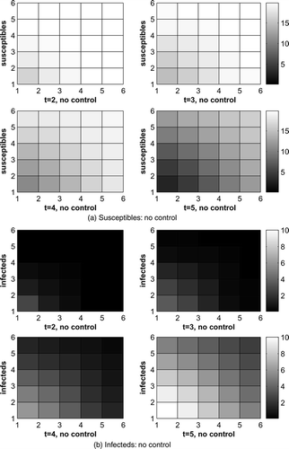
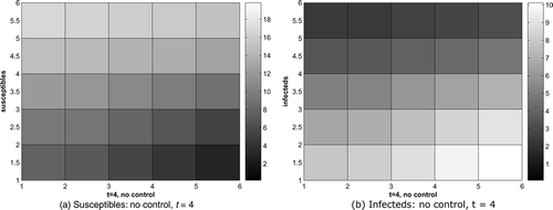
First we give the numerical results without any control for time t = 2 to t = 5. Figure 1 shows the susceptible and infected raccoons without control. The disease spreads from the lower left corner to the upper right corner with the infected raccoons rapidly increasing.

Figure 1. Susceptible and infected raccoons, without control.

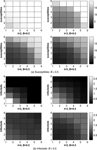
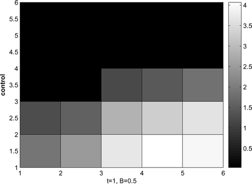
Figure 2 shows the susceptible and infected raccoons with optimal control and cost coefficient B = 0.5. The infected raccoons are reduced very efficiently.

Figure 2. Susceptible and infected raccoons, B = 0.5.

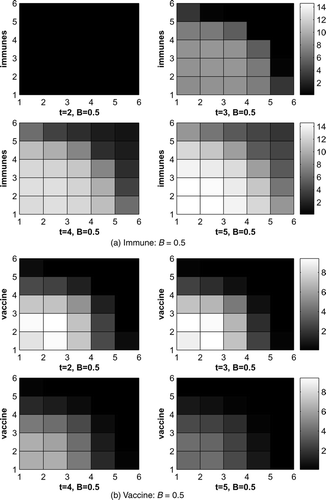
Figure 3 shows the immune raccoons and optimal vaccine distribution. Vaccination efforts decrease as time goes on. Notice we do not have any immune raccoons when t = 2 because we assume that no vaccine baits are already present at the initial time. The control adds baits at time t = 1 and those baits are in the vaccine variable at time t = 2, which influences the vaccine at t = 3 and so on. See equation (4).

Figure 3. Immune raccoons and vaccine distribution, B = 0.5.

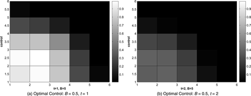
We also did the calculation for a much higher cost coefficient B = 5. In this case, we can still control the disease efficiently, but not as well as when B = 0.5 because it is much more expensive.

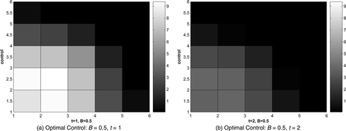
The optimal control for B = 0.5 and B = 5 are shown in figures 4 and 5. Only graphs for time t = 1 and t = 2 are given here. In the beginning, control focuses on the area where the infected raccoons are initially introduced and devotes more effort to the front of the disease. Similar patterns arise for both values of B, but with large difference in magnitude due to the greater expense to apply any control when B = 5. Notice no control is added in the final time step, which is due to the transversality condition (15) and the control characterization (8).

Figure 4. Optimal control, B = 0.5, t = 1, 2.

Figure 5. Optimal control, B = 5, t = 1, 2.

The same results arise when the disease starts from one of the other three corners of the grid.

4.2 Disease starts from the middle

As another scenario, assume the susceptibles are homogeneously distributed with 20 in each cell except at the center of the grid, where we introduce 4 infected raccoons, and keep 16 susceptibles there. Notice it only takes one time step for the disease to spread everywhere.

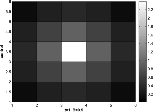
The optimal control for t = 1 and B = 0.5 is shown in figure 6. Control effort is focused on the area where the infected raccoons are initially introduced, then the effort is reduced on the adjacent cells, with no control applied for times t = 2, 3. The focus is on stopping the disease where it happens, which is different from the strategy when the disease starts from the corner.

Figure 6. Optimal control, disease starts in the middle, B = 0.5.

4.3 Inhomogeneous initial distribution

For a third scenario, we double the infected raccoons in the lower right corner relative to those in the lower left corner. So initially susceptibles are homogeneously distributed with 20 in each cell except at these two corner cells, we introduce 8 and 4 infected raccoons, respectively, and keep 12 and 16 susceptibles there.

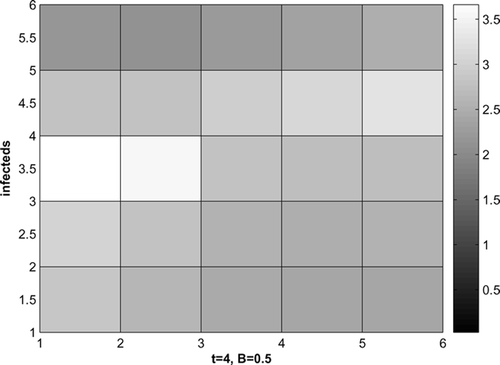
Figure 7 gives the susceptible and infected raccoons without control for t = 4, with more infected raccoons spreading from the lower right corner. With control, figure 8 shows the infected raccoons with the cost coefficient B = 0.5. The infecteds can be reduced effectively by about two-thirds.

Figure 7. Susceptible and infected raccoons, without control, disease starts at 2 corners, t = 4.

Figure 8. Infected raccoons, disease starts at 2 corners, B = 0.5, t = 4.

The optimal control for t = 1 and B = 0.5 is given by figure 9. Control is applied to the lower right corner where there are more infected raccoons. More effort is applied to nearby cells on the bottom row than to the corner cells to prevent the spread of rabies from the two sources.

Figure 9. Optimal control, disease starts at 2 corners, B = 0.5, t = 1.

4.4 Discussion on the effects of parameter change

We also calculated our results for a variety of different parameter values. If we increase e ₁, which is the effectiveness of the vaccine to a susceptible raccoon eating a bait, then the immune raccoons increase because more susceptibles move to the immune class; also the control effort increases and keeps the same pattern, e.g. if the disease starts from the corner, more effort concentrates on the front of the disease rather than right at that corner. If we increase e ₂, which is the (weighted) consumption rate of the vaccine taken by the susceptible and immune raccoons, the vaccine decreases and so does the immunes. Note that e ₂ cannot be large, otherwise there will no vaccine dynamics, as the vaccine only equals the additional baits added. If e ₂ is large, many baits are consumed so that the only baits at time t + 1 are from the baits added by time t. When the transmission rate β decreases, the control effort also decreases. Since the β term is proportional to the fraction of the infecteds, the β cannot be very small, otherwise the disease is not able to spread and no control effort is needed. If we increase the size of the grid N, it takes a longer time to run the code but the same pattern occurs; in this case, we need to increase the initial population size to ensure the disease spreads out.

5. Conclusion

Our objective has been to develop a method and model to determine different optimal distributions of vaccine to control rabies spread. We illustrate the approach using three scenarios: two different disease start locations with a homogeneous initial distribution and a heterogeneous initial distribution. The control results show how the optimal bait distribution depends on the initial location of the disease outbreak and the distribution of raccoons throughout the grid. If the disease starts from a corner, more control is applied around that corner than exactly on the corner to prevent the spread of the disease. If the disease starts in the center, with more directions to spread, more control is applied at the start location. If the disease starts from two corners and one has more infecteds than the other, control is applied to prevent the two sources coming to meet each other.

The results here are relatively simple implementations to illustrate the methods and applications to very basic disease distributions. The method can be readily extended to evaluate optimal vaccination distribution strategies with other spatially heterogeneous interactions, larger spatial grids, and different movement assumptions. For example, information about details of the landscape which affect raccoon movement can be accounted for through spatially varying movement matrices. The method can also be applied to determine how robust vaccination strategies are to uncertainties in vaccination effectiveness, transmission rates and other parameters. Given the difficulty in estimating transmission rates from field data, models such as this are potentially very useful in determining whether these rates greatly impact the effectiveness of different disease management strategies.

Acknowledgements

This work was supported by National Science Foundation (NSF) Award ITR: 0427471 and National Institutes of Health (NIH) grant R01 AI047498 to LAR. We thank Scott Duke-Sylvester for helpful discussions related to this work. We also thank Scotta Ward and Kendall Ivie for their preliminary work on this model.

References

- Division of Viral and Rickettsial Diseases (DVRD) . Rabies , From National Center for Infectious Diseases (NCID) web site concerning rabies (http://www.cdc.gov/ncidod/dvrd/rabies/). Centers for Disease Control and Prevention
- USDA Wildlife Services . National Rabies Management Program , From USDA Animal and Plant Health Inspection Service web site concerning the National Rabies Management Program (http://www.aphis.usda.gov/ws/rabies/). USDA Animal and Plant Health Inspection Service
- Kallen , A. , Arcuri , P. and Murray , J. D. 1985 . A simple model for the spatial spread and control of rabies . Journal of Theoretical Biology , 116 : 377 – 393 .
- Murray , J. D. , Stanley , E. A. and Brown , D. L. 1986 . On the spatial spread of rabies among foxes . Proceedings of the Royal Society of London B , 229 : 111 – 150 .
- Evans , N. D. and Pritchard , A. J. 2001 . A control theoretic approach to containing the spread of rabies . IMA Journal of Mathematics Applied in Medicine and Biology , 18 : 1 – 23 .
- Coyne , M. J. , Smith , G. and McAllister , F. E. 1989 . Mathematic model for the population biology of rabies in raccoons in the mid-Atlantic states . American Journal of Veterinary Research , 50 : 2148 – 2154 .
- Allen , L. J.S. , Flores , D. A. , Ratnayake , R. K. and Herbold , J. R. 2002 . Discrete-time deterministic and stochastic models for the spread of rabies . Applied Mathematics and Computation , 132 : 271 – 292 .
- Childs , J. E. , Curns , A. T. , Dey , M. E. , Real , L. A. , Feinstein , L. and Bjornstad , O. N. 2000 . Predicting the local dynamics of epizootic rabies among raccoons in the United States . Proceedings of the National Academy of Science , 97 : 13666 – 13671 .
- Russell , C. A. , Smith , D. L. , Childs , J. E. and Real , L. A. 2005 . Predictive spatial dynamics and strategic planning for raccoon rabies emergence in Ohio . Public Library of Science , 3 : 382 – 389 .
- Russell , C. A. , Smith , D. L. , Waller , L. A. , Childs , J. E. and Real , L. A. Proceedings of the Royal Society of London B . A priori prediction of disease invasion dynamics in a novel environment , Vol. 271 , pp. 21 – 25 .
- Smith , D. , Lucey , B. , Waller , L. A. , Childs , J. E. and Real , L. A. 2002 . Predicting the spatial dynamics of rabies epidemics on heterogeneous landscapes . Proceedings of the National Academy of Sciences , 99 : 3668 – 3672 .
- Asano , E. , Gross , L. J. , Lenhart , S. and Real , L. 2007 . Optimal control of vaccine distribution in a rabies metapopulation model , preprint
- Clark , C. 1990 . Mathematical Bioeconomics: The Optimal Management of Renewable Resources , (2nd edn) , Chichester : Wiley .
- Sethi , S. P. and Thompson , G. L. 2000 . Optimal Control Theory: Application to Management Science and Economics , Dordrecht : Kluwer .
- Hof , J. and Bevers , M. M. 2002 . Spatial Optimization in Ecological Applications , New York : Columbia University Press .
- Pontryagin , L. S. , Boltyanskii , V. G. , Gamkrelize , R. V. and Mishchenko , E. F. 1962 . The Mathematical Theory of Optimal Processes , Chichester : Wiley .
- Lenhart , S. and Workman , J. T. 2007 . Optimal Control Applied to Biological Models , Boca Raton : CRC Press .