Optimal control applied to native–invasive population dynamics

Abstract

This article presents a model for population interactions between an invasive and a native species, where the effect of disturbance in the system (such as flooding) is modeled as a control variable in the growth terms. The motivating example is cottonwood–salt cedar competition, with flooding being detrimental at low and high levels and being advantageous at medium levels, which led us to consider quadratic growth functions of the control. An objective functional is formulated to maximize the native species while minimizing the cost of implementing the control. A new existence result for an optimal control with these quadratic growth functions is given. Numerical results are examined for various parameter values. The results provide suggestions for managing the disturbance regime when invasive species are present.

Keywords:

• Optimal control
• Invasive species
• Population dynamics
• Salt cedar
• Cottonwood
• Eco-logical disturbance

1. Introduction

The problem of invasive, non-native species has become common in much of the world, in large part due to the introduction of new species by human beings, albeit sometimes accidentally. When developing successful plans for the eradication or control of invasives, the resulting dynamics must be considered 1–3. Human alterations to a local environment can alter the interactions between two competing species, and should be taken into account when managing invasive species 4. A natural disturbance in the environment, such as fire or flood, is often detrimental to businesses, homes and agriculture. Therefore such disturbance is often restricted or prevented. However, native species may depend on this natural disturbance to grow and propagate.

An illustrative example of this occurs in the American southwest. Native cottonwood trees (such as Populus deltoides) have to contend with a number of invasive species; among the most prevalent are Tamarix ramosissima and several other members of the genus Tamarix, which are commonly known as tamarisks or salt cedars. Due to the low levels of rainfall in much of the region, cottonwood forests tend to dominate naturally only along rivers or other areas where there is surface water. Salt cedars, originally from central Asia andwestern China, were introduced into New Mexico in the 19th century, and to nearby regions at roughly the same time. Salt cedars were classified as an invasive species by the mid-twentieth century 5. They are more tolerant of drought, salinity, and fire than cottonwoods, all of which can occur when overbank flooding is restricted or eliminated 6. Currently, salt cedars occupy nearly every drainage system in arid and semi-arid areas west of the Great Plains, at minimum one million acres, and have been reported in about half of the eastern states of the United States 5.

For many years, the number of young cottonwood trees along rivers in the desert southwest has declined, with few if any young trees replacing the older ones. It has been suggested that salt cedars may competitively exclude cottonwood. However, recent studies have indicated that densities of cottonwood are not affected by the presence of salt cedar unless the densities of cottonwood are very low 6–9. While in many cases disturbance of an ecosystem allows an invasive species to become established, flooding is critical to the continuance of cottonwood forests. Current flood controls on large Southwest rivers, such as the Rio Grande, have allowed for an opportunistic invasion of salt cedars, which are far less affected by the conditions. Some studies have suggested that when the environment is allowed to return to a more natural state (especially with regard to flood control), the two species will co-exist, or the cottonwood will become the dominant species once again (see Stromberg 9, and Sher and Marshall 7).

Disturbances such as fire may be used to control an invasive species and to allow the native species to flourish 10–12. Unlike flooding, however, the timing and extent of fire is not always as advantageous to the native species. In the case of frequent fires, an invasive species can take advantage of an open space that fire can bring, and push out native species. Prescribed burns may still be necessary to prevent wildfires, but consideration needs to be taken that the ecosystem does not respond in the same way when invasives are present, and larger burns may now help invasive species substantially more than native ones 11. In other circumstances, a prescribed burn at an appropriate time of the year could be critical for preventing the spread of an invasive species, such as in Pollack and Kan's research on prescribed burns to control exotic annual grasses among native perennial grasses in California 12. Also see the works by Beckage et al. 13 for the responses of pine savannas to fire disturbances, and by Bond et al. 14 documenting the importance of fire in promoting the spread of grasslands and savannas.

We present a system of two ordinary differential equations (ODEs) to represent our competition model with a control acting on the growth terms; a key point is that the control affects each species differently. We note that ODE models can represent such competitions in plants or animals 16–19. The major goal here is to maximize the amount of the native species by applying the control action at appropriate times of year, while minimizing the ‘cost’ of implementing the control. This ‘cost’ may include the actual financial impact to carry out the management plan but also may consider the negative impact on the environment or economic development.

Motivated by the idea of ‘flooding’, which may be detrimental at low and high levels and advantageous at medium levels, we consider growth functions which are quadratic in the controls. A new control analysis result presented here develops the existence of an optimal control in the case of quadratic functions of the control appearing in both ODEs, under a restriction on the coefficients of the quadratics.

The model and optimal control formulation are introduced in the next section. We present the existence of optimal control results in section 3, along with the necessary conditions for solving this optimal control problem. The optimal control is characterized in terms of the adjoints and states. In the final section, we illustrate some numerical results for the cottonwood-salt cedar scenario and other situations and include some concluding remarks.

2. Model dynamics

The state variables in this model will be the population densities, rather than biomass, due to existing biological information for both inter- and intra-species competition. The general model for the population dynamics is given by

where are the intrinsic net growth rates (depending on the control u(·)), and a _ij are the interaction coefficients indicating how species j affects species i. We are using the convention that the N ₁ population is the (native) population that we want to grow by applying the control. Population N ₂ is the competitor (perhaps invasive) population. The initial population values G ₁ and G ₂ are known positive constants. The interaction coefficients a ₁₁, a ₁₂, a ₂₁ and a ₂₂ are assumed to be positive.

The control variable u(t) represents the amount of intervention at time t (in years). The control u has a pair of constraints. First, the control is scaled so that 0≤u≤1. More notably, we only allow the control action to take place during certain times of the year. Connecting back with our motivating example, we would only allow flooding in the spring thaw when cottonwoods release their seeds. Starting the year in the spring, this is taken to occur during the first tenth of each year. Similarly, prescribed burns may be done in the late spring just before seed dispersal, or right after the start of seasonal rains. For instance, Pollack and Kan 12 found that after carefully timed burns, medusahead, an exotic grass present in California's Central Valley, was dramatically reduced or eliminated while native species returned to dominance in every site examined.

Thus we define our control set to be

and

Here, is the characteristic function of the set Ω, which is given by

with T denoting the number of years of controls and interval being in the ith year. Then we see that on the set , the control does not appear in the state equation, which amounts to saying that the control does not apply during those time intervals.

The growth rate parameters of a ₁, b ₁, c ₁, a ₂, b ₂ and c ₂ are chosen to fit a specific scenario. In the cottonwood–salt cedar case, ecological research influences the choice of growth rates. Tallent-Halsell and Walker 15 noted that both insufficient and excessive water levels can severely affect the establishment rate of salt cedars. In spite of this, salt cedars are better able to tolerate drought than cottonwoods; the population density still can increase without excessive flooding, though it more likely comes from vegetative growth rather than seedlings. Sher et al. 6 8 found that flooding patterns similar to those present before the use of damming and other controls increased the establishment of cottonwood seedlings. Thus, the parameters are chosen so that with little or no flooding the salt cedar population, N ₂, has a higher growth rate than the cottonwood population, N ₁.

It should be noted that for other scenarios, the choice of growth rate parameters may be quite different. For instance, Brooks and Pyke 11 comment that regular, periodic fire in some ecosystems may allow for invasive species to become dominant, even in cases where fire is a natural occurrence and where native species are well-adapted to regular burns. In this circumstance, the growth parameters would instead be chosen so that the native population N ₁ has a higher growth rate in the absence of fire, but not for extensive burns.

Our objective functional to be maximized is given by:

where the first population is to be maximized at the final T subject to balancing the minimization of the second population and the cost of implementing the control. Many times the cost of implementing a control would be nonlinear and as such a simple nonlinear case is taken here. As mentioned the costs can include funds needed for control implementation as well as the negative financial impact on the environment. If one takes K=0, then the emphasis is to promote the first population without regard to the second population.

3. Existence of optimal controls and optimality system

The nonlinear state system with measurable coefficients as controls has a solution taking values in , due to a standard result in Lukes 20, and a priori L ^∞ bounds hold for the states from the structure of the system. Note that if the differential equations are linear in the control, i.e.

we can obtain the existence of an optimal control from standard results in Fleming and Rishel 21 since the integrand of the objective functional is concave, the control set is convex, and the range of the control values is compact.

However, in the case that the growth functions, , are quadratic in the control with a coefficient restriction, we must do some analysis to get the existence of an optimal control. To begin with, for any , let us denote

Then the state equation reads

and the payoff functional reads

Our main result of this section is the following theorem.

Theorem 3.1

Suppose there exists a κ≥0 such that

then there exists an optimal control u* in U with corresponding states , that maximizes the objective functional J(u) defined by (3).

Proof

For any , define

Our proof consists of two steps.

• Step 1. An optimal control exists if for almost all t∈[0, T] and each , the set is convex and closed.

  We are going to sketch the proof for this step (see chapter 3 of 23 for details).

• Step 2. The set is convex and closed.

For this part, condition (4) will play an important role.

Now, we present a sketch of the proof for Step 1. Let be a maximizing sequence and N ⁿ (·) be the state trajectory corresponding to u ⁿ (·). Then one can show that the sequence is uniformly bounded and equicontinuous. Hence, we may assume that

By the definition of , one has

Next, by the boundedness of N ⁿ (·), we have the L ²(0, T) weak convergence of to some . Then Mazur's theorem 22 (together with Egorov's Theorem) yields that for any , there exists an , such that (where is the Lebesgue measure of )

for some , . On the other hand, for any δ>0,

where is the δ-neighborhood of set A. The above is because uniformly, and is convex. Then

Here, we have used the closedness of . Since is arbitrary, we obtain

Then, by the definition of we obtain

and

Since

there exists a such that

Then is the state trajectory corresponding to the control and

Thus, is an optimal control.

Now, we present a proof for Step 2. The closed property is obvious, since is continuous. For the convexity, we note that (4) yields

Clearly, when ,

is trivially convex. Hence we now consider t∈Ω. Denote . Since κ≥0, , for u∈[0, 1]. Thus, is convex, monotone increasing, and

which is convex. Consequently, f(t, N, [0, 1]) is convex. Now, for any and , we have some u, v∈[0, 1] such that

By the convexity of and (5), we can find some w∈[0, 1] such that

which leads to

By the monotonicity of , we have from the first inequality in (6) that

Further, from the equality in (6), we see that

Hence, in the case that κ>0, (note (4), (8) and (9))

In the case that κ=0, (9) becomes

which leads to (by the convexity of u↦ u ²)

Hence, we obtain

proving the convexity of .

We now use Pontryagin's Maximum Principle 24 to find the optimal control. First we formulate the Hamiltonian from the cost functional (3) and the governing dynamics (1),

where λ₁ and λ₂ are the associated adjoints for states N ₁ and N ₂, respectively. The adjoint variables will be needed to calculate the optimal control. The system of equations is found by taking the appropriate partial derivatives of the Hamiltonian (10) with respect to the associated state variable.

Theorem 3.2

Given an optimal control u* and corresponding states , , there exists adjoint functions satisfying

with transversality conditions

Furthermore, the characterization holds:

Proof

To calculate the adjoint differential equations, we use

On the interior of the control set, we have

Taking into account the control bounds, we obtain the desired characterization of u*.    ▪

Thus the optimality system consists of the state system (1), together with the adjoint system (11) and associated transversality boundary conditions (12), coupled with the characterization of the optimal control. We now examine the population changes for a variety of parameter values and growth functions, including our cottonwood–salt cedar scenario.

4. Numerical illustrations and conclusions

In computing the optimal control and state values, the following algorithm was used. An initial estimate for the control is made. The state variables are then solved forward in time from the dynamics (1) using a Runge Kutta method of the fourth order. Resulting state values are placed in adjoint equations (11). These adjoint equations with given final conditions (12) are solved backwards in time, again employing a fourth order Runge Kutta method. Both state and adjoint values are used to update the control, and then the process is repeated. This iterative process terminates when current state, adjoint, and control values converge sufficiently. Numerical results were completed for a variety of parameter values and theta functions, including the cottonwood–salt cedar case. Note that condition (4) is verified in each numerical example.

4.1 Quadratic growth functions

In the cottonwood–salt cedar scenario, quadratic growth functions can represent reasonable qualitative behavior for newly established seedling communities. The interaction coefficients, a _ij , express how species j affects species i. Sher et al. 8 found that cottonwood density affects the population of both species (in a negative fashion) more than the salt cedar density. In fact, salt cedar density does not seem to affect the population size of cottonwoods except when the cottonwood density is much smaller than the salt cedar density. Thus a ₁₂ is very small and a ₂₁>a ₂₂. For the numerical illustration, the interaction parameter values are:

To model the cottonwood–salt cedar scenario, we choose when u=0 and we use our quadratic growth functions,

We assume that the two seedling populations start with equal densities, so our initial conditions are scaled to be G ₁=G ₂=1. When u=0, the growth functions are 0 and 0.2, respectively. The cottonwood density decreases, while the salt cedar density increases without any flooding; see figure 1.

Figure 1. With no control: cottonwood–salt cedar scenario.

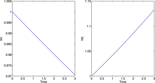
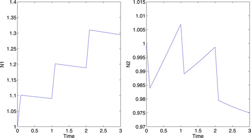
Consider the case A=9, B=2.5, ε=7, and K=0, in which we are concentrating on the cottonwood population and our goal does not directly involve the salt cedar population. To correspond with the spring thaw, flooding is only allowed during the first 1/10 of the year for a period of 3 years. In figure 2, the optimal control does not get close to the maximum u value, due to the cost of implementing the control. If we decrease the cost coefficients, B and ε, the optimal control values are greater. The optimal control allows for the cottonwood density to increase but remain approximately equal to the salt cedar density. If we were to apply maximum control, u=1, during the first 1/10 of the year for a period of 3 years, the salt cedar density would see a decline; see figure 3. With 3 consecutive years of flooding in the spring, cottonwoods are able to dominate salt cedars. Taylor et al. 25 show that under such conditions, the cottonwoods will continue to dominate beyond the sapling stage, thereby forming a dominant canopy species. A dominant cottonwood canopy should further limit the growth rate of salt cedar.

Figure 2. Optimal control: cottonwood–salt cedar scenario.

Figure 3. Cottonwood–salt cedar scenario with maximum control.

4.2 Quadratic growth functions: alternative scenario

Again N ₂ is a population which is typically dominated by the N ₁ population, but because of the absence of some control, N ₁ has diminished and N ₂ has increased. In contrast to the cottonwood–salt cedar case, we now let N ₂ have a competitive advantage over N ₁, meaning, a ₁₂>a ₂₁. Our interaction parameters are:

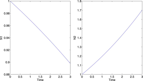
Using the same growth functions as that in 4.1, we will again start with equal population size, G ₁=G ₂=1. With no control, the growth rates of N ₁ and N ₂ are 0 and 0.2, respectively. See figure 4 for populations without control.

Figure 4. With no control: alternative quadratic growth scenario.

In subsection 4.1, we allowed the control to be applied for 1/10 of a year. However, the control may have longer-lasting effects. Suppose the control is applied during the first quarter of each year for 3 years. Let . The numerical results are displayed in figure 5. The presence of the control significantly increases the N ₁ growth rate, and promotes a reasonable proportion between the two populations.

Figure 5. Optimal control: alternate quadratic growth scenario with K=1.

4.3 Linear growth functions

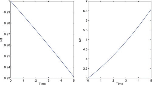
For some scenarios, linear growth functions may be a better representation. Consider a situation where the lack of control has allowed N ₂ to become the dominant species. We will assume u=1 is the level of control which maximizes growth in the native species N ₁. For the linear growth rates, we again assume when u=0. For these examples, we will use these model parameters:

Without control, N ₂ increases and N ₁ decreases; see figure 6. To include minimizing N ₂(T) as part of our goal, we allow K>0. Our parameters are now

Again, we allow control to be applied only during the first 1/10 of each year. The optimal control is displayed in figure 7. Because of the positive K value in our objective functional, the optimal control decreases during the last years to keep N ₂(T) small. Overall, the N ₁ population increases by over 30%. If the control can be applied for a longer interval of time during each year, we need fewer years to achieve more drastic results. For example, see figure 8 for optimal control using the same parameters as above, but with T=3 and control applied during the first 3/4 of year. After 3 years of control, N ₁ is clearly the dominating species once again.

Figure 6. With no control: linear growth functions scenario.

Figure 7. Optimal control: linear growth functions scenario.

Figure 8. Optimal control: linear growth functions with longer control period.

4.4 Concluding remarks

This work demonstrates that optimal control theory can be an appropriate tool for designing intervention strategies to control an invasive species. We were able to prove existence results for an optimal control in certain quadratic cases in the growth functions. In those quadratic cases and in linear cases for the growth functions, we were able to numerically compute various scenarios for different interaction coefficients. Other forms of interaction terms (not involving the controls) may be used, including predator–prey scenarios and various functional responses. Note also our set-up allowed for controls that acted in only part of the year.

We have obtained novel existence results of optimal controls for certain structures of growth functions. Difficulty in proving existence results arises in the terms involving the controls, due to the fact that maximizing sequences of controls only converge weakly. In the future, we may continue to explore what forms of growth functions will give further existence results.

Acknowledgements

This work was supported by National Science Foundation Award No. ITR: 0427471. We thank Louis Gross, Mike Fuller, Nina Tallent-Halsell, Jaffar Ali Shahul-Hameed, Wandi Ding and Mike Saum for helpful discussions related to this work.

References

- Myers , J. H. , Simberloff , D. , Kuris , A. M. and Carey , J. R. 2000 . Eradication revised: dealing with exotic species . TREE , 15 : 316 – 320 .
- Lodge , D. M. 1993 . Biological invasions: lessons for ecology . TREE , 8 : 133 – 137 .
- Shigesada , N. and Kawasaki , K. 1997 . Biological Invasions: Theory and Practice , New York : Oxford University Press .
- Peters , D.P. C. , Bestelmeyer , B. T. , Herrick , J. E. , Fredrickson , E. L. , Monger , H. C. and Havstad , K. M. 2006 . Disentangling complex landscapes: new insights into arid and semiarid system dynamics . Bioscience , 56 : 491 – 501 .
- Westbrooks , R. 1998 . Invasive Plants: Changing the Landscape of America: Fact Book , Washington, D.C. : Federal Interagency Committee for the Management of Noxious and Exotic Weeds, U.S. Dept of the Interior .
- Sher , A. A. , Marshall , D. L. and Gilbert , S. A. 2000 . Competition between Populus deltoides and invasive Tamarix ramoisissima and the implications for reestablishing flooding disturbance . Conservation Biology , 14 : 1744 – 1754 .
- Sher , A. A. and Marshall , D. L. 2003 . Seedling competition between native Populus deltoides (Salicaceae) and exotic Tamarix ramoisissima (Tamaricaceae) across water regimes and substrate types . American Journal of Botany , 90 : 413 – 422 .
- Sher , A. A. , Marshall , D. L. and Taylor , J. P. 2002 . Establishment patterns of native Populus and Salix in the presence of invasive Tamarix . Ecological Applications , 12 : 760 – 772 .
- Stromberg , J. 1998 . Dynamics of Fremont cottonwood (Populus fremonti) and saltcedar (Tamarix chinensis) populations along the San Pedro River, Arizona . Journal of Arid Environments , 40 : 133 – 155 .
- Jameson , D. A. 1982 . Effects of burning on a Galleta–Black Grama range invaded by Juniper . Ecology , 43 : 760 – 763 .
- Brooks , M. L. and Pyke , D. A. 2001 . Invasive plants and fire in the deserts of North America . Proceedings of the Invasive Species Workshop: The Role of Fire in the Spread and Control of Invasive Species. Fire Conference 2000: The First National Congress on Fire Ecology, Prevention, and Managemen . 2001 . Edited by: Galley , K.E. M. and Wilson , T. P. pp. 1 – 14 . Tallahassee, FL : Tall Timbers Research Station . Miscellaneous Publication No. 11
- Pollack , O. and Kan , T. 1998 . “ The use of prescribed fire to control invasive exotic weeds at Jepson Prairie Preserve ” . In Ecology, Conservation, and Management of Vernal Pool Ecosystems (1996) , Edited by: Witham , C. W. , Bauder , E. T. , Belk , D. , Ferren , W. R. Jr. and Ornduff , R. 241 – 249 . Sacramento, CA : Proceedings California Native Plant Society .
- Beckage , B. , Gross , L. J. and Platt , W. J. 2006 . Modeling responses of pine savannas to climate change and large-scale disturbance . Applied Vegetation Science , 9 : 75 – 82 .
- Bond , W. J. , Midgley , G. F. and Woodward , F. J. 2003 . The importance of CO-2 and fire in promoting the spread of grasslands and savannas . Global Change Biology , 8 : 973 – 982 .
- Tallent-Halsell , N. G. and Walker , L. R. 2002 . Responses of Salix Gooddingii and Tamarix Ramoissima to flooding . WETLANDS , 22 : 776 – 785 .
- Vandermeer , J. H. 1989 . The Ecology of Intercropping , Cambridge : Cambridge University Press .
- Tilman , D. 1988 . Plant Strategies and the Dynamics and Structure of Plant Communities , Princeton : Princeton University Press .
- Courchamp , F. and Caut , S. 2005 . “ Use of biological invasions and their control to study the dynamics of interacting populations ” . In Conceptual Ecology and Invasions Biology , Edited by: Cadotte , M. W. , McMahon , S. M. and Fukami , T. 253 – 279 . Berlin : Springer .
- Murray , J. D. 2002 . Mathematical Biology I: An Introduction , New York : Springer-Verlag .
- Lukes , D. L. 1982 . Differential Equations: Classical to Controlled , New York : Academic Press .
- Fleming , W. H. and Rishel , R. W. 2005 . Deterministic and Stochastic Optimal Control , New York : Springer-Verlag .
- Yosida , K. 1980 . Functional Analysis , Berlin : Springer-Verlag .
- Li , X. and Yong , J. 1995 . Optimal Control Theory for Infinite Dimensional Systems , Boston : Birkhäuser .
- Pontryagin , L. S. , Boltyanskii , V. G. , Gamkrelize , R. V. and Mishchenko , E. F. 1967 . The Mathematical Theory of Optimal Processes , New York : Wiley .
- Taylor , J. P. , Smith , L. M. and Haukos , D. A. 2006 . Evaluation of woody restoration in the middle Rio Grande: ten years after . WETLANDS , 26 : 1151 – 1160 .