Abstract
A model is introduced for the transmission dynamics of a vector-borne disease with two vector strains, one wild and one pathogen-resistant; resistance comes at the cost of reduced reproductive fitness. The model, which assumes that vector reproduction can lead to the transmission or loss of resistance (reversion), is analyzed in a particular case with specified forms for the birth and force of infection functions. The vector component can have, in the absence of disease, a coexistence equilibrium where both strains survive. In the case where reversion is possible, this coexistence equilibrium is globally asymptotically stable when it exists. This equilibrium is still present in the full vector–host system, leading to a reduction of the associated reproduction number, thereby making elimination of the disease more feasible. When reversion is not possible, there can exist an additional equilibrium with only resistant vectors.
1. Introduction
Since the pioneering work of Ross in the late 19th and early 20th centuries Citation1 Citation2, the classical approach for controlling vector-borne diseases involves the eradication or strict population control of the vectors. In the case of malaria, for instance, sanitization, drainage of mosquito breeding grounds and the use of insecticides have long proved effective in reducing the number of human cases. However, the total eradication of the vector population is not always feasible, nor is it always desirable to put it in effect in practice. There is increasing resistance to insecticides in vectors Citation3 and insecticides may be harmful to other species. Furthermore, there are issues concerning the reduction of biodiversity (vectors are part of the food chain) and uncertainties about alternatives (if a given type of vector disappears, pathogens might evolve to utilize other species).
Because the elimination of vectors is difficult in practice (and may not be ecologically desirable), other control methods must be used simultaneously to effectively control the spread of the disease. For many vector-borne infections, no long-term immunization methods are available for the hosts and other options, such as prophylactic measures preventing contacts between vectors and hosts, are often employed. If a vector has several host species that are affected by the pathogen, then the efficacy of prophylactic measures is greatly diminished. Also, prophylactic measures require permanent compliance from the hosts.
Another approach to the fight against vector-borne diseases is based on using the natural resistance (or refractoriness) of the vectors to the pathogens. In the case of malaria, among the about 430 known species in the genus Anopheles, the mosquito vector, only a limited number (30–40) are vectors of Plasmodium, the parasite causing the disease. This parasite has a complicated life cycle within the mosquito. The normal cycle of the parasite is as follows (see, e.g. [Citation4, ]). During a blood meal on an infected host, the female mosquito ingests gametocytes, which then become successively gametes and zygotes. After about 24 h, ookinetes invade the gut, and differentiate into oocysts. The oocysts rupture after about 2 weeks, giving sporozoites, which then invade the salivary gland and can subsequently infect another host. In resistant vectors, encapsulation is detected: Plasmodium ookinetes are coated with a melanin-like substance, after traversing the gut wall Citation5. This substance consists of lamellocytes, which are large flat cells that are part of the primitive immune system of insects. These cells form a capsule around the ookinetes, isolating, immobilizing and ultimately, killing them Citation6. Encapsulation thus inhibits transmission of Plasmodium to humans or other hosts. Elucidating the origins of this resistance has long been an active research topic. A promising avenue of research has been opened by progress in genetic engineering Citation7, as vectors can be genetically altered to express resistance to Plasmodium (see, for instance, Citation4 Citation8 Citation9). For this purpose, mosquitoes are genetically transformed with transposable elements, resulting in a reduced ability to transmit the disease, but with a fitness cost. The reduced fitness of transgenic mosquitoes prevents the efficient spread of their genes in the wild vector population. Hence, understanding the conditions required for the spread of pathogen-resistance in the vector population is an important issue.
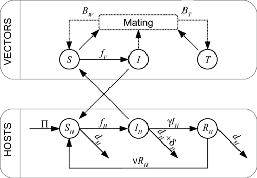
Figure 1. Flow diagram of the model. The upper box describes flows within the vector states, the lower box represents flows within the host states. The flows between boxes are the cross infection effects. The logistic-type dynamics of the vectors is not represented.
Mathematical models for vector-borne diseases have been studied for a long time; see, e.g. Citation10–12 and the references therein. Models coupling genetic aspects to epidemiology are considered, e.g. in Citation13. Finally, pathogen-resistance, its transmission and impact on disease prevalence has been studied in Citation14 Citation15. In line with the latter works, the model presented here has two main objectives:
-
(i) to study the propagation of resistance in a population of wild vectors that interbreed with an introduced type that is resistant to a given pathogen; and
-
(ii) to study the epidemiological consequences of the presence of pathogen-resistant vectors on the transmission dynamics of a vector-borne disease.
2. Modeling
2.1 Hypotheses
The population of vectors under consideration is divided into two types: a wild (natural) type, denoted by W, and a type that is resistant to the pathogen, denoted by T. The working hypotheses of the model are as follows.
-
H1 Resistant vectors are completely immune to the pathogen.
-
H2 a A proportion p 1 of the offspring resulting from the interbreeding of wild and resistant vectors are resistant to the pathogen.
-
H2 b A proportion p 2 of the offspring resulting from inbreeding within the resistant type are resistant to the pathogen.
-
H3 In the absence of disease, wild vectors are better fitted for competition than resistant vectors.
-
H4 Wild vectors are ill-fitted for competition when they carry the disease.
These hypotheses are now discussed in the context of malaria, where a significant amount of work has been carried out; they are however general enough to be applicable to any vector-borne diseases in which a mechanism of resistance of vectors can exist (for instance, dengue and yellow fevers).
H1 is a simplifying hypothesis motivated by experimental observations. In Citation5, for example, the resistance of various strains of Anopheles gambiae is quantified, by counting the number of encapsulated ookinetes present in the guts of lines of resistant mosquitoes and mosquitoes susceptible to the pathogen. It is observed that in the resistant strain, almost all ookinetes are encapsulated, as opposed to none for the susceptible strain.
In the case of malaria, one mechanism used to induce and propagate resistance is through transposable elements. The latter can be considered as mobile DNA sequences that are able to colonize the genome of their host by inserting new copies of themselves in it (transposition). Existence of non-Mendelian mechanisms such as the regulation of the rate of transposition, deletion (loss of copies) and genetic recombinations allow to consider loss of resistance and non-systematic resistance transmission Citation16, accounted for in the model by H2 b and H2 a , respectively.
Note that H2 makes a phenomenological description of the propagation of resistance to the offspring; the precise mechanisms that lead to inheritance of the resistant phenotype are not explicitly modeled. Also, when considered in conjunction with H1, hypothesis H2 can be interpreted as follows: a vector is resistant if its load in resistance-causing genetic material is sufficient. A vector that does not have enough of this material is considered susceptible.
Hypothesis H3 also stems from biological observations. Insertions of new copies of transposable elements can damage the genome if, for instance, insertion takes place into a coding sequence. For example, in the case of Aedes aegypi (a mosquito transmitting yellow fever), Citation17 finds a severe reduction in the net reproductive rate, with the control strain exhibiting a net reproductive rate 42–72% higher than that of the three transgenic strains it studies. These effects on fitness are confirmed by many other studies; see, e.g. Citation18–22.
Finally, H4 is a modeling hypothesis. Although there is still some debate about the precise effect on vectors Citation23, and a great deal of variability depending on the parasite and vector strains Citation24, some studies document reduced fertility of Plasmodium-infected mosquitoes (fertility being one component of fitness). Plasmodium yoelii nigeriensis is shown in Citation25 to reduce overall fertility of Anopheles stephensi by between approximately 40 and 50%. In Citation26, the mean egg production is found to be significantly lower for Anopheles gambiae infected with Plasmodium falciparum than for uninfected ones. In Citation27, it is shown that when competing (without interbreeding), resistant mosquitoes win the competition in the presence of Plasmodium, and wild mosquitoes win the competition in the absence of Plasmodium. Reduced fitness of infected vectors is also observed for other pathogen–vector pairs; see, e.g. Citation28.
2.2 Vector demography
Wild vectors can have two epidemiological states, susceptible (denoted by S) or infected (denoted by I), whereas resistant vectors are denoted by T. By H1, resistant vectors are totally immune to the pathogen. The simplifying assumption of a constant sex ratio is made.
In the following sections,
2.2.1 Birth and transmission of resistance
Associated with the numbers of vectors of each state, there are birth functions b
i
(X, Y). These functions describe the formation pairs and the resulting rate of birth. Assuming symmetry of the birth functions, i.e. , there are six different types of pairings, hence six birth functions b
i
, i=1, …, 6; see .
Table 1. Reproduction hypotheses: types of pairings, birth functions and mating outcomes.
The progeny belong to the different states. Since it is assumed that there is no vertical transmission, newborns can either be susceptible (wild) or resistant. Depending on the type of parents, a certain fraction of the newborns are resistant, and the remaining fraction are susceptible wild. For simplicity, transmission of resistance is assumed independent of disease status, for the wild-type vectors. This gives the mating outcomes in , which account for H2 a and H2 b .
At this point, the functional forms of the b i 's are not specified. However, it is assumed that they are of the same nature for all types of pairings, and that they satisfy the so-called pair-formation properties Citation29–31, as detailed below.
The birth functions and type of offspring are put together in the type-specific birth functions B W (S, I, T) and B T (S, I, T) for wild and resistant vectors, given, respectively, by
-
PF1
,
-
PF2
-
PF3
-
PF4
Consequently, the total birth function also satisfies properties PF1–. Additionally, it is assumed that B(S, I, T) satisfies the following hypothesis,
-
PF5 There exist
2.2.2 Vector dynamics
Motivated by a logistic formulation where the population has a linear net growth rate and is subject to a quadratic competition term, the vector dynamics in the absence of new infections is governed by the following system:
For a given vector type X∈{W, T}, the net growth represents the difference between the net birth rate B X and the net natural per-capita death rate d X . Since there is no vertical transmission of the disease, all the birth into the wild type occurs in S with type-specific rate B W .
The parameters and κ
T
represent the rates of competition-induced mortality for susceptible wild, infective wild and resistant vectors, respectively. Note that the κ
X
's should in fact be κ
XY
's, rates of mortality of state X when competing with state Y. However, for simplicity, it is assumed that competition affects a given state at the same rate, regardless of the state of its competitor. Evidence of the effect of crowding is given, for example, by Citation32 and references therein.
Finally, infected vectors suffer additional disease-induced death at a per-capita rate δ W (see, e.g. Citation22 Citation33 in the case of malaria).
This system is not logistic in a strict sense, but in the proof of Theorem 2.1, it is shown that the total vector population is almost logistic.
2.2.3 Considerations on fitness
To account for hypothesis H3, it is assumed that resistance comes at the cost of reduced fitness. Furthermore, infection reduces fitness (H4). The precise definition of fitness in assumptions H3 and H4 is difficult to give. It is supposed, as in Citation9 Citation14 Citation22, that being fit describes a set of attributes that makes the vector better suited for survival.
Reproductive fitness is taken into account by ranking the associated fecundities, with the most fecund vectors being the susceptible wild, followed by the resistant, and the least fecund being the infected wild vectors. For each mating pair, it is assumed that fecundity is always determined by the less fit of the pair. As a consequence, for given appropriate (X, Y), the functions b i (X, Y)'s can be ordered as follows for positive population values
Similar to the birth functions, the rates of competition-induced mortality are partially ordered to account for vector fitness. Susceptible wild vectors are better fitted than both infectious wild and resistant, but the latter two cannot be ordered a priori, so
Finally, the natural death rate, d
T
, for resistant vectors includes the cost of resistance ().
2.3 Host demography
The demography for hosts is supposed to follow a simple SIRS model. The hosts are susceptible (S H ), infective (I H ) or recovered (R H ). Birth occurs into the state S H at the constant rate Π, and death at the per-capita rate d H in all states. Upon infection, susceptible individuals proceed to the infective state, where they are subject to disease-induced death with per-capita rate δ H . The sojourn time in the infective state is exponentially distributed with mean 1/γ, giving the per-capita rate γ of moving from the I H to the R H state. In the R H state, individuals are immune to infection. The duration of the immune period is exponentially distributed with mean 1/ν.
Note that this is a crude simplification of the dynamics of most vector-borne diseases. In the case of malaria, for example, a realistic model Citation11 categorizes humans into eight different epidemiological states. However, SIRS models capture some of the essential mechanisms in the transmission of a disease without the burden of additional parameters and nonlinearities. Furthermore, the analysis here can be extended in a straightforward way to models with a latent state (such as those in Citation11).
2.4 Force of infection
Assume that the rate of infection of a susceptible host by an infected vector is f H , and the rate of infection of a susceptible vector by an infected host is f V . These functions aggregate two different processes: vector bites, which represent the contacts, and transmission of the disease. The force of infection f H depends directly on S H and I, while f V depends directly on S and I H . In accordance with H1, there is no direct dependence on T. Both f V and f H can, however, depend indirectly on T, through dependence on the total vector population V. They might also depend on the total host population H.
In its most general formulation, the model uses generic forms for f H and f V , assuming that the following hypotheses are satisfied:
-
(i) f V and f H are C 1;
-
(ii) f V ≥0 and f H ≥0;
-
(iii)
-
(a) f V =0 if either S=0 or I H =0;
-
(b) f H =0 if either S H =0 or I=0.
-
2.5 The model
The model, taking into account the above hypotheses, is given below (see for a schematic diagram and for a description of parameters and variables).
Table 2. Model variables and parameters, and assumptions on parameter values. Note that all parameters are assumed positive unless otherwise stated in the text
3. Some general properties of the system
Define composite parameters b, ,
, r,
,
,
, K and
as in .
Theorem 3.1
The total vector population V(t) is such that, for all t≥0,
Proof
First, it is clear that the positive orthant is invariant under the flow of Equation(4)
. As a consequence, V(t)>0 and H(t)>0, for all t≥0, for positive V(0) and H(0). The total vector population V in system Equation(4)
satisfies
Now summing the equations for hosts gives
Thus the vector component of system Equation(4) is almost logistic, in the sense that, from Equation(8)
, the evolution of the total vector population is bounded by two logistic equations. From now on, it is assumed that the maximal intrinsic growth rate
. This is a natural assumption, since it implies that wild vectors are present in the absence of disease or competition.
The next result about reproduction numbers for system Equation(4) is obtained using the method of Citation34. The present model is one case where this method must be applied carefully.
Theorem 3.2
Consider a disease-free equilibrium of
Equation(4)
taking the form
Proof
In the absence of disease, the vector population is V=S+T and
Note that Theorem 3.2 does not address uniqueness of the disease-free equilibrium. In fact, the disease-free equilibrium is not in general, unique, as exemplified in the special case of sections 4 and 5. In the case of multiple disease-free equilibria, ℛ should be defined for each equilibrium at which Theorem 2.2 can be applied. Further analysis is then required to determine parameter regions where the disease might go extinct or persist in the population.
Also note that caution should be used when applying Theorem 3.2. Condition (A5) states that the system without disease must have its spectrum to the left of the imaginary axis. In section 5, it is shown that this is not always true; refer to the discussions following Theorems 5.1, 5.2 and 5.3 for details.
4. Special case—vectors only and no disease
In order to investigate the first objective of the paper (potential coexistence of the two vector types, wild and resistant), system Equation(3) is considered using a specific functional form for the birth functions.
In this special case, it is assumed that birth obeys the following law. First, for vectors of the same state ,
-
(i)
-
(ii)
-
(iii)
-
(iv)
-
(v)
4.1 Coexistence of vectors
The first question concerns the possibility for both vector types (wild and resistant) to coexist, in the absence of disease. System Equation(4) with only noninfectious vectors reduces to
The existence of an additional equilibrium point and the stability of the various equilibria are determined by the following theorem.
Theorem 4.1
The extinction equilibrium Ē 0 is always unstable. Additionally, suppose that p 2<1. Then:
-
(a) If
-
(b) If
Interpretation
𝔽
S
is a characteristic of the wild species in the absence of disease. measures the relative fitnesses of wild and resistant vectors in the absence of disease and interbreeding. If the fitness advantage of wild vectors relative to resistant vectors decreases past a threshold, then the resistant vectors become established in the population. This threshold,
, is the contribution to resistance from interbreeding.
Proof
Conditions for the existence of the coexistence equilibrium Ē C are established in Appendix B.
At Ē
0=(0, 0), i.e. in , the Jacobian matrix Df takes the form
Table
When Ē
C
exists, that is, if , Ē
W
is unstable. Using the Dulac function
on the vector field f, the divergence of the Jacobian takes the form
When Ē C does not exist, then Ē W is locally asymptotically stable and using the same argument, is globally asymptotically stable. ▪
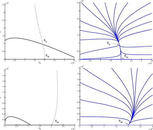
shows nullclines of Equation(15). Using notations as in Appendix B, the nullcline of Equation(15a)
is the curve Γ
S
=0, represented by a dashed line. The nullcline of Equation(15b)
consists of the curve Γ
T
=0 (the parabolic arc joining both axes, shown as a continuous line), together with the S-axis. The coexistence equilibrium Ē
C
, when it exists, lies at the intersection of the curves Γ
S
=0 and Γ
T
=0 (top left figure). In the case of the figure on the bottom, a transcritical bifurcation has taken place at the point where Γ
S
=0 and Γ
T
=0 coincide on the S-axis. As the curve Γ
S
=0 moves to the right (this is achieved here by increasing α1), the equilibrium Ē
C
at the intersection of Γ
S
=0 and Γ
T
=0 exchanges stability with Ē
W
(and becomes irrelevant biologically).
Figure 2. Left column: nullclines of Equation(15a) (Γ
S
=0, dashed lines) and Equation(15b)
(Γ
T
=0, continuous line), in the case p
2<1, as in section 4.1. Right column: a few corresponding sample solutions. First row: case 1 in Theorem 4.1, where 𝔽
S
−𝔽
T
<(p
1α5/κ
T
) (both Ē
W
and the coexistence equilibrium Ē
C
exist, Ē
C
is globally asymptotically stable). Second row: case 2 in Theorem 4.1, where 𝔽
S
−𝔽
T
≥(p
1α5/κ
T
) (only Ē
W
exists, and is globally asymptotically stable).
Note that Theorem 4.1 implies that at Ē
C
, when it exists, both eigenvalues of have negative real parts, which is used in Theorem 4.2.
4.2 Another equilibrium can exist when there is no loss of resistance
Suppose now that p 2=1, i.e. there is no loss of resistance in the offspring of two resistant parents. Additionally to Ē 0, Ē W and, when it exists, Ē C , the additional equilibrium is found
Theorem 4.2
Ē 0 is unstable. Suppose that p 2=1. Then the existence and stability of the equilibria Ē W , Ē C and Ē T are summarized in the following table.
Table
Interpretation
Here, the mating of T vectors always leads to T offspring. This hypothesis can be interpreted as an absence of reversion, i.e. resistance cannot be lost. In this case, if the fitness of resistant vectors is positive, another situation with only resistant vectors becomes possible. When the fitness of resistant vectors relative to the fitness of wild-type vectors is very large, then the outcome of competition is the presence of only resistant vectors. For lower values of the fitness of resistant vectors, the situation is very similar to that of the case with reversion (Theorem 4.1). See .
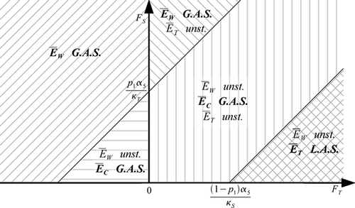
Figure 3. Regions of existence and stability of the various equilibria, in the absence of disease, in the wild and resistant fitness plane, as given by Theorem 4.2 (p 2=1).
Proof
The instability of Ē 0 is proved as before. It is possible here to compute explicitly the value of the coexistence equilibrium. Using Maple, and after some manipulations, it is found that at Ē C ,
The regions in the -plane that are deduced from Theorem 4.2 are illustrated in .
4.3 The competitive exclusion principle holds in the absence of interbreeding
From Theorem 4.1, both wild and resistant vector strains can coexist in the absence of disease. This is quite different from the standard context of competition models, where the competitive exclusion principle usually holds. This principle states that the species that is most adapted to survival when resources are low, survives the competition, and all others become extinct. Intuitively, the coexistence must stem here from interbreeding.
To ascertain this, consider now system Equation(15) without interbreeding of vectors (α5=0) or reversion (p
2=1),
Theorem 4.3
System
Equation(15)
with α5=0 and p
2=1, i.e. system Equation(17)
, has three equilibria, Ē
0, Ē
W
and Ē
T
, with Ē
0
and Ē
T
unstable, and Ē
W
globally asymptotically stable.
Proof
The same three equilibria Ē 0 and Ē W (section 4.1), and Ē T (section 4.2), are found. At the origin, eigenvalues are
Note that this conclusion is very similar to that drawn in Citation27. Indeed, suppose a reversed fitness situation, as would be the case in the presence of disease. Then the resistant vectors become established, driving the wild ones extinct.
5. Special case—disease dynamics in the full system
To address the second objective of the paper, namely, to assess the effect of resistance on the transmission dynamics, the full six-dimensional system Equation(4) is now considered.
5.1 Force of infection
Let be the rate at which bites are received by a single host per unit time. Let c
2 be the per-capita biting rate of vectors (on a host); for simplicity, assume that, within the population of interest, c
2 is a constant. This is a justified assumption; for mosquitoes, for example, the female has a certain number of blood meals over its lifetime.
For the number of bites to be conserved (that is, the total number of vector bites all hosts get equals the total number of bites made by all vectors), the following relation must hold:
5.2 The model
With the assumptions on the birth and force of infection functions, system Equation(4) takes the form
5.3 Analysis—case of no intervention
In order to assess the effect of resistant vectors, the behavior of the system in the absence of resistant vectors, i.e. when T≡ 0, is first studied. This describes the disease dynamics in its natural setting, without any outside intervention. From PF4, setting T=0 in Equation(19c) implies that T remains identically zero in Equation(19)
. Recall that in the absence of disease, the vector and host subsystems decouple. In this case, there are two equilibria for the vector component, one with S=0, Ē
0, and another with
, Ē
W
. To each of these two-vector equilibria corresponds the unique disease-free equilibrium for the host component, S
H
=Π/d
H
. As a consequence, in the vector–host system, there are two equilibria [Etilde]0 and [Etilde]
W
without disease. Proceeding as in the proof of Theorem 3.2, the following theorem can be established, which gives the basic reproduction number
in the absence of resistant vectors.
Theorem 5.1
For system
Equation(19)
without resistant vectors (T≡ 0), there are two disease-free equilibria. The equilibrium
Proof
At the equilibrium [Etilde]0, the Jacobian matrix has the eigenvalues ,
, −d
H
,
, −(d
H
+ν) and
, giving the instability of [Etilde]0. The expression of Equation(20)
and the stability of [Etilde]
W
is a direct application of Theorem 3.2 with T≡ 0. ▪
Remark that it is not possible to use Theorem 3.2 at [Etilde]0, since [Etilde]0 is always unstable even in the system without disease, implying that assumption (A5) in Theorem 3.2 does not hold.
5.4 Analysis—full system
The disease-free equilibria of the full system Equation(19) are the equilibria found for the simplified system Equation(15)
with only vectors studied in section 4, together with the equilibrium without disease for the hosts component.
Thus, the equilibria [Etilde]0 and [Etilde] W (as given in Theorem 5.1) are the equilibria with no vectors and only the wild vectors present, respectively. Also, when they exist,
Theorem 5.2
[Etilde]0 is always unstable. Additionally, if p 2<1, then:
-
(a) If
-
(b) If
Interpretation
This is similar to the situation with no disease and only vectors. The effect of resistant vectors on the disease dynamics is shown in particular in Case (a), where there is coexistence of both types. The disease cannot go extinct without intervention, since [Etilde]
W
, the equilibrium for the disease in its natural setting, is unstable, but could potentially be brought to extinction if . Note that the results obtained are only local, implying a possibility of control of the disease, not a certain outcome.
Proof
The instability of [Etilde]0 is established in Theorem 4.1. The conditions for existence of [Etilde] W and [Etilde] C are the same as in Theorem 4.1.
-
Case (a). The stability of [Etilde] C follows from Theorem 3.2. At [Etilde] W , there is an unstable manifold of dimension at least equal to 1, corresponding to the unstable manifold of dimension 1 of Ē W found in the case
-
Case (b). The stability of [Etilde] W is considered in Theorem 5.1. ▪
Note that in Case (a), the system without disease, which decouples into independent components for vectors and hosts, has its vector component governed by Case (a) in Theorem 4.1: when Ē
C
exists, Ē
W
is unstable. This implies that in this case, in the absence of disease [Etilde]
W
is always unstable, so condition (A5) of Theorem 3.2 is not fulfilled at [Etilde]
W
, and as defined by Theorem 3.2 plays no role in determining the stability of [Etilde]
W
.
Theorem 5.3
[Etilde]0
is unstable. Suppose that p
2=1. Firstly, if
, then the existence and stability of the equilibria [Etilde]
W
, [Etilde]
C
and [Etilde]
T
is summarized in the following table:
Table
Table
Interpretation
In the case where there is no reversion, resistant vectors can only invade the population if their fitness advantage over the wild vectors is sufficiently large. Note that the fitness advantage required for resistant vectors to have the possibility of invading the vector population in this case, is the same as the one required in the absence of disease (as given by Theorem 4.2).
Proof
Remark that is the condition for existence of Ē
T
in Theorem 4.2, and as a consequence, of [Etilde]
T
. Suppose now that [Etilde]
T
exists. At [Etilde]
T
, the Jacobian matrix takes the form
It is interesting to note that Theorem 3.2 cannot be applied to [Etilde]
T
. Indeed, ordering the variables as , it follows that when evaluated at [Etilde]
T
, the block in the jacobian matrix corresponding to the variables S, T is
The last result concerns the relationship between the basic reproduction numbers in the natural setting and
with resistant vectors. As remarked earlier, these two numbers cannot be defined simultaneously in the context of Theorem 3.2. It is, however, possible to compare the expressions obtained when both equilibria exist simultaneously, without considerations on stability.
Theorem 5.4
At the coexistence equilibrium [Etilde] C , when it exists, there holds that
Interpretation
If conditions are such that the resistant vectors can coexist with the wild vectors, then the potential for effective control of the disease is better than in the natural case.
Proof
Suppose that [Etilde]
C
exists. The expression for is then obtained using Theorem 3.2. Also, there holds that
. Indeed, using the notations of Appendix B,
. This implies that, using the expression for Γ
S
=0,
6. Discussion
In this paper, an ordinary differential equations model for the spread of pathogen resistance in the vectors of a vector-borne disease is formulated. Two vector types are considered: wild and resistant. A phenomenological description of pathogen-resistance inheritance is incorporated: the two types interbreed, and a given proportion of the offspring of resistant vectors are resistant. It is also assumed that resistance comes at the cost of a reduced fitness, which is modeled by supposing that resistant vectors have lower reproduction rates and higher rates of natural and competition-induced mortalities. It is proved that:
-
(i) The spread of pathogen resistance in the vector population is possible in the absence of disease. This is established by analyzing the vector only system in the absence of disease (Theorems 4.1 and 4.2).
-
(ii) Pathogen resistence of the vectors leads to a reduction of the reproduction number, thereby making control of the disease potentially more feasible (Theorem 5.4).
Mathematically, the model also has interesting features. The existence of up to four disease-free equilibria is quite unusual. This is due to the multiple nonlinearities that are present even in the absence of disease. To circumvent the difficulties inherent to these nonlinearities, it was necessary to use ideas from projective geometry to show the existence and uniqueness of the co- existence equilibrium. Another interesting characteristic is the fact that, contrary to many models, it is here not always possible to use the result of Citation34 to estimate the basic reproduction number and its influence on the local asymptotic stability of disease-free equilibria. It appears that, at a given point in parameter space, Theorem 3.2 can only be used at one of the disease-free equilibria, namely, the one that is globally stable. Whether this is a feature of the present model, or a more general characteristic of the method of Citation34, raises interesting mathematical questions.
This paper is a preliminary work. The modeling of resistance and its inheritance should be made more realistic. Also, the model is complicated and some of the more challenging mathematical aspects have not been tackled. The existence of endemic equilibria in the full, six-dimensional case, is a hard problem, and is left untouched here. Also, it is not certain that in the cases and
, the disease indeed goes extinct (Theorem 5.2 is a local result). Numerical simulations seem to indicate that such is the case, but so far this fact is not proved.
Acknowledgements
We are greatly indebted to Claudio Struchiner for introducing us to the subject of Transposable Elements, and for comments on earlier versions of the manuscript. We acknowledge expert help for the proof of the existence part of Theorem 4.1 from Bernard Gibert, and discussions with P. van den Driessche and James Watmough about the next generation technique. Four anonymous referees of two different versions of this paper provided helpful comments. The work of JA, AB and SP is supported in part by NSERC. JA and AB are also supported in part by MITACS.
References
- Ross , R. 1905 . The logical basis of the sanitary policy of mosquito reduction . Science , 22 ( 570 ) : 689 – 699 .
- Ross , R. 1905 . Researches on malaria , London : John Bale, Sons & Danielsson . Nobel Prize lecture, available from: http://nobelprize.org
- Brogdon , W. G. and McAllister , J. C. 1998 . Insecticide resistance and vector control . Emerging and Infectious Diseases , 4 ( 4 ) : 605 – 613 .
- Riehle , M. A. , Srinivasan , P. , Moreira , C. K. and Jacobs-Lorena , M. 2003 . Towards genetic manipulation of wild mosquito populations to combat malaria: advances and challenges . Journal of Experimental Biology , 206 : 3809 – 3816 .
- Collins , F. H. , Sakai , R. K. , Vernick , K. D. , Paskewitz , S. , Seeley , D. C. , Miller , L. H. , Collins , W. E. , Campbell , C. C. and Gwadz , R. W. 1986 . Genetic selection of a Plasmodium-refractory strain of the malaria vector Anopheles gambiae . Science , 234 : 607 – 610 .
- Osta , M. A. , Christophides , G. K. , Vlachou , D. and Kafatos , F. C. 2004 . Innate immunity in the malaria vector Anopheles gambiae: comparative and functional genomics . Journal of Experimental Biology , 207 : 2551 – 2563 .
- Aultman , K. S. , Beaty , B. J. and Walker , E. D. 2001 . Genetically manipulated vectors of human disease: a practical overview . TRENDS in Parasitology , 17 ( 11 ) : 507 – 509 .
- Christophides , G. K. 2006 . Transgenic mosquitoes and malaria transmission . Cellular Microbiology , 7 ( 3 ) : 325 – 333 .
- Struchiner , C. J. , Kidwell , M. G. and Ribeiro , J. M.C. 2005 . Population dynamics of transposable elements: copy number regulation and species invasion requirements . Journal of Biological Systems , 13 ( 4 ) : 455 – 475 .
- Antonovics , J. , Iwasa , Y. and Hassell , M. P. 1995 . A generalized model of parasitoid, venereal, and vector-based transmission processes . American Naturalist , 145 ( 5 ) : 661 – 675 .
- Dietz , K. , Molineaux , L. and Thomas , A. 1974 . A malaria model tested in the African savannah . Bulletin of WHO , 50 : 347 – 357 .
- Rogers , D. J. 1988 . The dynamics of vector-transmitted diseases in human communities . Phil. Trans. R. Soc. Lond. B , 321 : 513 – 539 .
- Fischer , C. , Jock , B. and Vogel , F. 1998 . Interplay between humans and infective agents: a population genetic study . Human Genetics , 102 : 415 – 422 .
- Boëte , C. and Koella , J. C. 2002 . A theoretical approach to predicting the success of genetic manipulation of malaria mosquitoes in malaria control . Malaria Journal , 1 ( 3 )
- Koella , J. C. and Boëte , C. 2003 . A model for the coevolution of immunity and immune evasion in vector-borne diseases with implications for the epidemiology of malaria . American Naturalist , 161 ( 5 ) : 698 – 707 .
- Le Rouzic , A. and Capy , P. 2005 . The first steps of transposable elements invasion: parasitic strategy vs. genetic drift . Genetics , 169 : 1033 – 1043 .
- Irvin , N. , Hoddle , M. S. , O'Brochta , D. A. , Carey , B. and Atkinson , P. W. 2004 . Assessing fitness costs for transgenic Aedes aegypti expressing the GFP marker and transposase genes . PNAS , 101 ( 3 ) : 891 – 896 .
- Boëte , C. and Koella , J. C. 2003 . Evolutionary ideas about genetically manipulated mosquitoes and malaria control . TRENDS in Parasitology , 19 ( 1 ) : 32 – 38 .
- Catteruccia , F. , Godfray , H. C.J. and Crisanti , A. 2003 . Impact of genetic manipulation on the fitness of Anopheles stephensi mosquitoes . Science , 299 : 1225 – 1227 .
- Hurd , H. , Taylor , P. J. , Adams , D. , Underhill , A. and Eggleston , P. 2005 . Evaluating the costs of mosquito resistance to malaria parasites . Evolution , 59 ( 12 ) : 2560 – 2572 .
- Roy , B. A. and Kirchner , J. W. 2000 . Evolutionary dynamics of pathogen resistance and tolerance . Evolution , 54 ( 1 ) : 51 – 63 .
- Yan , G. , Severson , D. W. and Christensen , B. M. 1997 . Costs and benefits of mosquito refractoriness to malaria parasites: implications for genetic variability of mosquitoes and genetic control of malaria . Evolution , 51 ( 2 ) : 441 – 450 .
- Ferguson , H. M. and Read , A. F. 2002 . Why is the effect of malaria parasites on mosquito survival still unresolved? . TRENDS in Parasitology , 18 ( 6 ) : 256 – 261 .
- Ferguson , H. M. , Rivero , A. and Read , A. F. 2003 . The influence of malaria parasite genetic diversity and anaemia on mosquito feeding and fecundity . Parasitology , 127 : 9 – 19 .
- Jahan , N. and Hurd , H. 1997 . The effects of infection with Plasmodium yoelii nigeriensis on the reproductive fitness of Anopheles stephansi . Annals of Tropical Medicine and Parasitology , 91 ( 4 ) : 365 – 369 .
- Hogg , J. C. and Hurd , H. 1997 . The effects of natural Plasmodium falciparum infection on the fecundity and mortality of Anopheles gambiae s.l. in north east tanzania . Parasitology , 114 : 325 – 331 .
- Marrelli , M. T. , Li , C. , Ragson , J. L. and Jacobs-Lorena , M. 2007 . Transgenic malaria-resistant mosquitoes have a fitness advantage when feeding on Plasmodium-infected blood . PNAS , 104 ( 13 ) : 5580 – 5583 .
- Lee , J.-H. , Rowley , W. A. and Platt , K. B. 2000 . Longevity and spontaneous flight activity of Culex tarsalis (Diptera: Culicidae) infected with Western equine encephalomyelitis virus . Journal of Medical Entomology , 37 ( 1 ) : 187 – 193 .
- Castillo-Chavez , C. and Huang , W. 1995 . The logistic equation revisited: the two-sex case . Mathematical Biosciences , 128 : 299 – 316 .
- Dietz , K. and Hadeler , K. P. 1988 . Epidemiological models for sexually transmitted diseases . Journal of Mathematical Biology , 26 : 1 – 25 .
- Hsu Schmitz , S.-F. and Castillo-Chavez , C. 2000 . A note on pair-formation functions . Mathematical and Computer Modelling , 31 : 83 – 91 .
- Ng'habi , K. R. , John , B. , Nkwengulila , G. , Knols , B. G.J. , Killeen , G. F. and Ferguson , H. M. 2005 . Effect of larval crowding on mating competitiveness of Anopheles gambiae mosquitoes . Malaria Journal , 4 ( 49 )
- Anderson , R. A. , Knols , B. G. and Koella , J. C. 2000 . Plasmodium falciparum sporozoites increase feeding-associated mortality of their mosquito hosts . Anopheles gambiae s.l. Parasitology , 120 : 329 – 333 .
- van den Driessche , P. and Watmough , J. 2002 . Reproduction numbers and sub-threshold endemic equilibria for compartmental models of disease transmission . Math. Biosci. , 180 : 29 – 48 .
- Gyllenberg , M. and Metz , J. A.J. 2001 . On fitness in structured metapopulations . Journal of Mathematical Biology , 43 ( 6 ) : 545 – 560 .
- Metz , J. A.J. , Nisbet , R. M. and Geritz , S. A.H. 1992 . How should we define ‘fitness’ for general ecological scenarios? . Trends in Ecology and Evolution , 7 ( 6 ) : 198 – 202 .
- Ngwa , G. A. and Shu , W. S. 2000 . A mathematical model for endemic malaria with variable human and mosquito populations . Mathematical and Computer Modelling , 32 : 747 – 753 .
- Li , J. 2004 . Simple mathematical models for interacting wild and transgenic mosquito populations . Mathematical Biosciences , 189 : 39 – 59 .
- Coolidge , J. L. 1931 . A Treatise on Algebraic Plane Curves , Oxford : Oxford University Press .
- Bronshtein , I. N. , Semendyayev , K. A. , Musiol , G. and Muehlig , H. 2004 . Handbook of Mathematics , 4 , Berlin : Springer .
Appendix A: Hypotheses for the van den Driessche and Watmough method
To compute reproduction numbers for a general epidemic model x′=f(x), with , Citation34 suppose that it is written in the form
-
(A1) If x≥0 then
-
(A2) If x i =0, then
-
(A3)
-
(A4) At a disease-free equilibrium,
-
(A5) If
Appendix B: Proof of the existence part of Theorem 4.1
Proof
To find nontrivial equilibria, suppose that Equation(15) is at equilibrium and multiply both equations by S+T. This gives equations for the nullclines for Equation(15a)
,
-
first, show that Θ=0 consists of two lines,
-
if
-
if
-
-
to lift this indetermination, turn to Γ T =0 and show that
-
either Γ T =0 does not intersect the first quadrant (no CEP),
-
or Γ T =0 intersects the first quadrant with two positive intercepts (CEP),
-
or Γ T =0 is a parabolic arc containing the origin (undetermined),
-
-
in the latter case, the line of Θ=0 through the first quadrant is shown to intersect Γ S =0 (CEP).
If , then a
1
a
2>0, implying that the lines L
1 and L
2 have slopes with the same sign, which is the same as the sign of a
1+a
2. Rewriting the terms in a
1+a
2 gives
If }, it follows that a
1
a
2<0, implying that L
1 and L
2 have slopes with opposite signs. In the rest of the proof, assume, without loss of generality, that L
1 is the line that intersects the first quadrant.
Study of Γ
T
The origin belongs to the curve Γ
T
=0. An algebraic calculation shows that, provided , Equation(B2)
is a parabola in the coordinate system rotated of an angle 3π/4. Also, there always holds that
, so that the parabola always opens towards the fourth quadrant of the (S, T)-plane. There are three cases.
If both intercepts are negative, there is no intersection of the conic section with the positive quadrant and thus there are no positive equilibria (and the boundary equilibrium Ē
T
is not feasible). This gives the condition (
) in the part 2 of the theorem.
If both intercepts are positive, the intersection of the conic section defined by Γ T =0 with the positive quadrant of the (S, T)-plane consists in a concave down parabolic arc between both intercepts. There is one point of intersection between Γ T =0 and L 1 in the positive quadrant.
If only is positive, then the intersection of Γ
T
=0 with the positive quadrant consists in the concave down parabolic arc joining
to the origin, and so the intersection with L
1 is undetermined (there might not be an intersection, if the slope of Γ
T
=0 at the origin were less than the slope of L
1).
Study of Γ
S
Use the cubic Γ
S
=0; letting T→∞ in Γ
S
=0 gives that is a vertical asymptote of Γ
S
, and it follows that Θ=0 intersects Γ
S
=0 in the positive quadrant. The first assertion in the theorem is proved, completing the proof of the existence part of Theorem 4.1. ▪