Multiple mixed-type attractors in a competition model

Abstract

We show that a discrete-time, two-species competition model with Ricker (exponential) nonlinearities can exhibit multiple mixed-type attractors. By this is meant dynamic scenarios in which there are simultaneously present both coexistence attractors (in which both species are present) and exclusion attractors (in which one species is absent). Recent studies have investigated the inclusion of life-cycle stages in competition models as a casual mechanism for the existence of these kinds of multiple attractors. In this paper we investigate the role of nonlinearities in competition models without life-cycle stages.

Keywords:

• Competitive exclusion principle
• Coexistence cycles
• Multiple attractors

1. Introduction

In 1 the authors utilize a competition model to explain an unusual coexistence result observed and studied by T. Park and his collaborators in a series of classic experiments involving two species of insects (from the genus Tribolium) 2–4. The explanation offered in 1 is based on a single species model (called the LPA model) designed explicitly to account for the dynamics of the species involved. The LPA model has an impressive track record, spanning several decades, of describing and predicting the dynamics of Tribolium populations, under a variety of circumstances in controlled laboratory experiments—dynamics that range from equilibrium and periodic cycles to quasi-periodic and chaotic attractors 5, 6. This history of success adds credence to the two-species competition model used in 1 (called the competition LPA model) and significant weight to the explanation given for the observed case of coexistence. The explanation entails, however, some unusual aspects with regard to classic competition theory, including non-equilibrium dynamics, coexistence under increased intensity of inter-specific competition, and the occurrence of multiple mixed-type attractors. By multiple mixed-type attractors we mean a scenario that includes at least one coexistence attractor and at least one exclusion attractor. A coexistence attractor is one in which both species are present. An exclusion attractor is one in which at least one species is absent and at least one species is present. Park observed the coexistence case in an experimental treatment that also included cases of competitive exclusion, that is to say, he observed a case of what we have termed to be multiple mixed-type attractors.

Competition theory is primarily an equilibrium theory that is exemplified, for example, by the classic Lotka–Volterra model and its limited number of asymptotic outcomes: a globally attracting coexistence equilibrium; a globally attracting exclusion equilibrium; or two attracting exclusion equilibria. (In this context, globally attracting means within the positive cone of state space.) These three equilibration alternatives are illustrated by the Leslie–Gower model 7 (the discrete analog of the famous Lotka–Volterra differential equation model)

where t=0, 1, 2, … and the b _i >0 are the inherent birth rates, s _i (0≤s _i <1) the survival rates, and c _ij >0 the density-dependent effects on newborn recruitment 8–10. Leslie et al. used this model to study the Tribolium experiments, but it is incapable of explaining the observed case of multiple mixed-type attractors. On the other hand, the competition LPA model used in 1 exhibits a greater variety of competition scenarios, including ones with multiple mixed-type attractors (also see 11, 12).

The competition LPA model, although applied specifically to species of Tribolium in 7, is none the less a rather general model that, unlike the Leslie–Gower model (or a Lotka–Volterra type model in general), accounts for life-cycle stages in the competing species. Therefore, the LPA model serves to illustrate that in general (when more biological details are included) competition theory is likely to be considerably more complicated and varied than that represented by classic Lotka–Volterra types of models. The competition LPA model is, like the Leslie–Gower model (1), a discrete-time (difference equation) model. It differs from the Leslie–Gower model, however, in two basic ways: the state variables of the LPA model account for three life-cycle stages for each species (which mathematically introduces time delays and makes the model higher dimensional) and it utilizes ‘stronger’ (overcompensatory) nonlinearities. A natural question to ask is which of these two mechanisms most accounts for non-Lotka–Volterra dynamic scenarios and, in particular, for the occurrence of multiple mixed-type attractors? With regard to the first mechanism, it is shown in 13 that a result of introducing only a single life-cycle stage (specifically, a juvenile stage) in just one species in a Leslie–Gower model (1) can indeed result in multiple mixed-type attractors—specifically, the occurrence of exclusion equilibria in the presence of coexistence 2-cycles (provided inter-specific competition is sufficiently strong). A more robust occurrence of multiple attractors (equilibrium and cycles) of mixed type occurs if both species are given a juvenile stage 14.

Our goal here is investigate the second mechanism, namely the role of the nonlinearity in the occurrence of multiple mixed-type attractors. We do this by introducing a Ricker-type nonlinearity into the Leslie–Gower model (1):

In section 2 we show that this Ricker competition model cannot display multiple equilibrium attractors of mixed type, a feature it therefore has in common with the Leslie–Gower model (1) and classic Lotka–Volterra theory. We will show in section 3, however, that the Ricker model (2) can exhibit scenarios with multiple mixed-type attractors in which periodic cycles are present. We provide formal proofs of this possibility (mathematical details appear in the Appendix) for the case of 2-cycle and equilibrium scenarios. An investigation for scenarios involving higher period cycles (or quasi-periodic or chaotic attractors) remains to be carried out, although we give in section 4 a numerical example involving higher period cycles and quasi-periodic attractors.

2. Equilibria

We can assume without loss in generality (by scaling the units of x and y) that c _ii =1 in the Ricker competition model (2). Therefore, we will consider, after relabeling c ₁₂ as c ₁ and c ₂₁ as c ₂, the competition model

The exclusion equilibria , of the Ricker competition model (3) are biologically feasible (i.e. lie on the positive axes) if and only if the inherent net reproductive numbers satisfy n _i >1. Besides the trivial equilibrium and these two exclusion equilibria, there exists only one other equilibrium:

The equilibrium E ₃ is a coexistence equilibrium if it lies in the positive cone . Let denote the unit square in R ².

Lemma 2.1

Assume (s ₁, s ₂)∈S. Let (x _t , y _t ) denote the solution of the Ricker competition model (3) with an initial condition (x ₀, y ₀) lying in the closure of . If n ₁<1 then . If n ₂<1 then .

Proof

If n ₁<1 then all solutions of the linear equation satisfy From the inequality and u ₀=x ₀, an induction shows for all t=0, 1, 2, …. A similar argument proves the assertion when n ₂<1.   ▪

We assume throughout the rest of the paper that both inherent net reproductive numbers satisfy n _i >1. In this case, all solutions of (3) are bounded and at least one species does not go extinct, as the following dissipativity and persistence theorem shows. The proof appears in the Appendix.

Theorem 2.1

Assume (s ₁, s ₂)∈S and both n _i >1 in (3). There exist positive constants such that all solutions with satisfy

The equilibrium w=ln n, n=b/(1−s), of

is (locally asymptotically) stable if . A period doubling bifurcation occurs as n increases through n ^cr . It follows that a necessary condition for the stability of an exclusion equilibrium E _i (i=1 or 2) of the competition equations (3) is that the inherent net reproductive numbers n _i satisfy

The linearization principle provides sufficient conditions for stability according to the magnitude of the eigenvalues of the Jacobian J(x, y) associated with (3) evaluated at an equilibrium point :

The Jacobians of the equilibria E _i , i=1 or 2, are triangular matrices whose eigenvalues appear along the diagonal. The equilibrium E _i , i=1 or 2, is hyperbolic if both eigenvalues

have absolute value unequal to 1 and, by the linearization principle 15, is (locally asymptoti-cally) stable if both have absolute value less than 1. Thus, a necessary condition that E _i be hyperbolic and stable is that

Sufficient for E _i to be hyperbolic and stable is that, in addition, the inequalities (5) hold.

Theorem 2.2

Assume (s ₁, s ₂)∈S, that one of the inequalities (7) holds, and that E ₃ is a coexistence equilibrium. Then E ₃ is unstable.

Proof

If one of the inequalities (7) holds and if E ₃ is a coexistence equilibrium, then the formula (4) for E ₃ implies 1−c ₁ c ₂<0. A calculation shows

The Jury criteria† for instability imply that at least one eigenvalue of J(x _e , y _e ) has magnitude greater than 1.   ▪

It follows from Theorem 2.2 that if at least one exclusion equilibrium is (hyperbolic and) stable, then either E ₃ is not a coexistence equilibrium or, if it is, it is unstable. Consequently, with regard to equilibria, a mixed-type multiple attractor scenario is impossible for the competition model (3). Thus, the Ricker competition model (3) and the classic Lotka–Volterra competition model have in common the impossibility of multiple mixed-type equilibrium attractors. In the next section we show, on the other hand, that it is possible for the Ricker model (3) to have multiple mixed-type non-equilibrium attractors.

3. Multiple mixed-type attractors

We want to investigate the possible occurrence of mixed-type non-equilibrium attractors in the Ricker model (3) under symmetrically high inter-specific competition (as has been observed in more complicated models that include juvenile life-cycle stages 1, 8, 11, 13, 14). To carry out this investigation by means of a single parameter problem, we introduce the notation , and re-write the competition model (3) as

Our goal is, for fixed birth rates b _i , survivorships s _i and competition ratio r, to investigate the existence and stability of non-equilibrium coexistence attractors as functions of the inter-specific competition intensity coefficient c. In this paper we restrict attention to coexistence 2-cycles. The source of these coexistence 2-cycles will be a competitive exclusion 2-cycle, that is to say, a 2-cycle on a coordinate axis that undergoes a loss of stability.

In the absence of species x _t the dynamics of species y _t are governed by the Ricker model equation

A period doubling bifurcation occurs at the critical value of b ₂ at which point the equilibrium y=ln n ₂ equals . This bifurcation results in a (locally asymptotically) stable 2-cycle

for b ₂ greater than but near

which we write as . The two points , of the 2-cycle (10) satisfy the equations

This 2-cycle is stable (by the linearization principle) because the product of the derivative of the map (9) evaluated at and at is less than one in absolute value, i.e.

holds under (11).

The 2-cycle (10) yields an exclusion 2-cycle

of the Ricker competition model (8). This 2-cycle is stable on the (invariant) y-axis under the assumption (11). Our first goal is to study the stability of this exclusion 2-cycle in the $x,y$-plane and determine how it depends on the competition intensity c. Specifically, we will show a planar loss of stability occurs at a critical value c* of c, the result of which is a (transcritical) bifurcation of non-exclusion 2-cycles.

By the linearization principle, the exclusion 2-cycle (13) is (locally asymptotically) stable if the spectral radius of the matrix is less than one. A calculation shows this matrix is triangular and its eigenvalues are

Under the assumption (11), (see (12)). As a function of c, the first eigenvalue is decreasing and satisfies

It follows that there exists a unique c*>0 such that .

Theorem 3.1

Assume (s ₁, s ₂)∈S and that is such that (9) has a stable 2-cycle. Let c* denote the unique positive root of the equation

The exclusion 2-cycle (13) of the competition model (8) is (locally asymptotically) stable for c>c* and unstable for c<c*.

The loss of stability of the exclusion 2-cycle (13) described in Theorem 3.1 suggests the occurrence of a bifurcation of planar 2-cycles from the exclusion 2-cycle (13). 2-Cycles of the map defined by (8) correspond to fixed points of the composite map. The point , corresponding to the exclusion 2-cycle (13), is a fixed point of the composite for all values of c. On the other hand, a positive fixed point of the composite corresponds to a coexistence 2-cycle. Positive fixed points of the composite satisfy the equations (obtained from the composite equations after x and y are cancelled)

where

Note that by the way that c* is defined, the point still satisfies these equations when c=c*, i.e. and . The Implicit Function Theorem implies the existence of a solution branch of equations (15) that passes through this point, i.e. a branch such that , provided the Jacobian of f and g with respect to x and y is non-singular when evaluated at . It is difficult in general to relate this non-singularity condition in a simple way to the para-meters b _i and s _i in the competition model (8). In the Appendix it is shown, however, that the non-singularity condition does hold for . The analysis utilizes the lowest order terms in Lyapunov–Schmidt expansions of the bifurcating exclusion 2-cycle (13), which in turn are then used to estimate the bifurcation value c* of the bifurcating 2-cycles generated by the solution branch . In that analysis, attention is restricted to b ₁ lying on the interval

For b ₁∈I the Ricker equation has a stable equilibrium.

Theorem 3.2

Assume (s ₁, s ₂)∈S and b ₁∈I. If , then a branch of coexistence 2-cycles bifurcates from the exclusion 2-cycle (13) at c=c*.

By Theorem 3.1, the exclusion 2-cycle (13) loses stability as c decreases through c*. By the exchange of stability principle (16, p. 26) the bifurcating coexistence 2-cycles guaranteed by Theorem 3.2 are (locally asymptotically) stable if they exist for (and unstable if they exist for ). Accordingly, our next goal is to determine the conditions under which the bifurcating coexistence 2-cycles occur for . That is to say, we want to determine when for the solution branch of equations (15). We can utilize the Lyapunov–Schmidt expansions used in the Appendix to establish Theorem 3.2 to calculate an expansion of c ^′(0) for b ₂ near , the lowest order terms of which determine the sign of c ^′(0). Details appear in the Appendix. To describe the results of this analysis, we need some further notation.

We partition the unit square into the union , where S ₁ is the set of points (s ₁, s ₂)∈S that satisfy either

and where S ₂ is the set of points (s ₁, s ₂)∈S that satisfy or satisfy

See figure 1. Two critical numbers , lying in the interval I and satisfying , are defined by (A10) and (A12) in the Appendix. Also defined in the Appendix, by formula (A11), is a critical value r* of the ratio r.

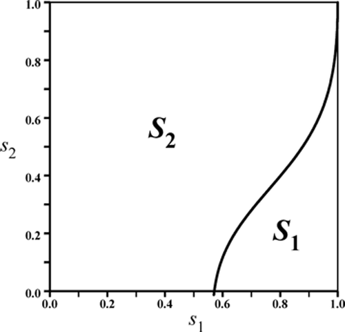
Figure 1. The unit square S for the survivorship parameters s ₁ and s ₂ in the competition model (8) is partitioned into to sub-regions S ₁ and S ₂ corresponding to the two case in Theorems 3.3.

Theorem 3.3

Assume b ₁∈I. For , and the bifurcating coexistence 2-cycles of the competition model (8) (guaranteed by Theorem 3.2 ) are stable in either of the following cases.

• (1)  and either

  • (a) 

  • (b)  and r<r*

  • (c)  and r<r*;

• (2)  and r<r*.

The subinterval in Theorem 3.4 is centered on the value

which supplies a rough estimate of those b ₁ for which the theorem applies.

According to (7), the exclusion equilibrium E ₁ is stable if

For it follows that and from Lemma A.3 in the Appendix that

Thus, if , then for and the inequality (16) holds and E ₁ is stable.

In order for both the coexistence 2-cycles and the exclusion equilibrium to be stable in the cases (1b,c) and (2) of Theorem 3.3, it is required that . Necessary for this requirement is This inequality is characterized in Lemma A.6 of the Appendix. These results, together with Theorem 3.3, lead to the following theorem.

Theorem 3.4

Assume b ₁∈I. For , and the exclusion equilibrium E ₁ and the bifurcating coexistence 2-cycles of the competition model (8) are both stable if and one of the following cases holds:

• (1) 

• (2)  and

• (3)  and .

This theorem provides conditions on the parameters in the competition model (8) under which there are multiple mixed-type attractors (specifically, a 2-cycle and an equilibrium). It follows from Lemma A.6 of the Appendix that in the cases not covered in Theorem 3.4 (namely when or when and b ₁ is near the endpoints 1−s ₁ and of the interval I) either the 2-cycle is unstable or the equilibrium E ₁ is unstable.

4. Discussion

The Ricker competition model (8) can possess multiple mixed-type attractors. Theorem 3.4 provides some conditions under which there exist both a stable exclusion equilibrium and a stable coexistence 2-cycle. That theorem deals with values of b ₂ greater than (but near) the critical period doubling bifurcation value , values of b ₁ less than the critical value , and with the inter-specific competition coefficient c near a specified critical value c*. The theorem also requires that the survivorships (s ₁, s ₂) lie in the region S ₁ of figure 1. 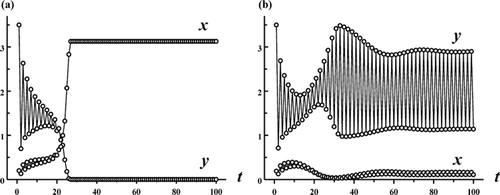This latter assumption means that the survivorship s ₁ of species x is larger than the survivorship s ₂ of species y. Therefore, Theorem 3.4 requires that there be an asymmetry between the two species in the sense that one species has a high reproductive rate and low survivorship in contrast to the other species, which has a low reproductive rate and a high survivorship. Figure 2 illustrates the existence of multiple mixed-type attractors under these conditions.

Figure 2. Each plot shows a solution of the Ricker competition model (8) with b ₁=8, b ₂=10, s ₁=0.65, s ₂=0, r=1.1 and c=1.9. In plot (a) the initial conditions (x ₀, y ₀)=(0.2, 3.5) lead to competitive exclusion. In (b) the initial conditions (x ₀, y ₀)=(0.19, 3.5) lead to a competitive coexistence 2-cycle. See figure 3(a).

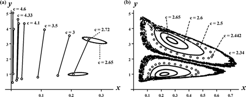
Theorem 3.4 implies the local bifurcation of stable coexistence 2-cycle only for c sufficiently large, namely, near the critical point c*. An interesting question concerns the global extent of this bifurcating branch of 2-cycles. What is the ‘spectrum’ of c values for which these coexistence 2-cycles occur? Numerous numerical explorations have shown that the bifurcation sequence displayed in figure 3 is typical. As c decreases, and the coexistence 2-cycles bifurcate from the exclusion 2-cycle on the y-axis at c=c*, there exists a second critical value of c at which the coexistence 2-cycles lose stability because of an invariant loop (Sacker/Neimark or discrete Hopf ) bifurcation. The resulting coexistence (double) invariant loops persist until c reaches a third critical value at which the loops disappear in a global heteroclinic bifurcation. See figures 3 and 4.

Figure 3. A sequence of phase plane plots shows the bifurcation of stable coexistence 2-cycles from the exclusion 2-cycles on the y-axis in the Ricker competition model (8) as the competition coefficient c decreases through the critical value c*≈2.35. Model parameters are b ₁=8, b ₂=10, s ₁=0.65, s ₂=0, and r=1.1. Plot (a) shows a sequence of stable 2-cycles (open circles with connecting lines) that eventually destabilize and give rise to stable, double invariant loops as shown in plot (b). In plot (c) the double invariant loops eventually collide, under further decreases in c, and undergo a global, heteroclinic bifurcation involving the (saddle) coexistence equilibrium, the exclusion (saddle) equilibrium, the exclusion (saddle) 2-cycle located and their stable and unstable manifolds. For the parameter values in these plots, the exclusion equilibrium E ₁:(x, y)≈(22.86, 0) is also stable and hence these plots contain multiple mixed-type attractors.

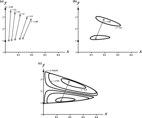
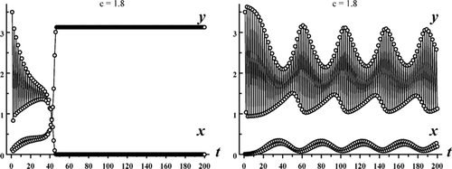
Figure 4. Each graph shows a solution of the Ricker competition model (8) with b ₁=8, b ₂=10, s ₁=0.65, s ₂=0, r=1.1 and c=1.8. In plot (a) the initial conditions (x ₀, y ₀)=(0.12, 3.5) lead to competitive exclusion. In plot (b) the initial conditions (x ₀, y ₀)=(0.01, 3.5) lead to a competitive coexistence quasi-periodic oscillation (see figure 3(b, c)).

In this paper we have shown that the Ricker competition model (8) cannot display a multiple mixed-type attractor scenario with only equilibria. On the other hand, Theorem 3.4 shows that multiple mixed-type attractor scenarios are possible with non-equilibrium attractors, specifically, with stable competitive exclusion equilibria and stable coexistence 2-cycles. Multiple mixed-type attractors scenarios are also possible for model (8) that involve other combinations of higher period cycles, quasi-periodic (as in figure 4) and even chaotic attractors. Figure 5 shows one example. The analysis of such multiple attractor cases remains an open problem.

Figure 5. A sequence of phase plane plots shows the bifurcation of stable coexistence 4-cycles from the exclusion 4-cycles on the y-axis in the Ricker competition model (8) as c decreases from the critical value c*≈4.77. Model parameters are b ₁=8, b ₂=14, s ₁=0.8, s ₂=0, r=0.8 and c=1.9. Plot (a) shows a sequence of 4-cycles the undergoes a period-halving bifurcation to 2-cycles which ultimately destabilize and give rise to stable, double invariant loops. As c decreases further, plot (b) shows the double invariant loops, which occasionally period lock, eventually giving rise to chaotic attractors. The chaotic attractors suddenly disappears when an ‘interior crisis’ occurs at a critical value of c. For the parameter values in these plots, the exclusion equilibrium E ₁:(x, y)≈(3.69, 0) is also stable and hence these plots contain multiple mixed-type attractors.

Acknowledgements

We thank R.F. Constantino, J. Edmunds, S.L. Robertson and S. Arpin for helpful discussions. J.M. Cushing and S.M. Henson were supported in part by NSF grant DMS-0414142.

Notes

^†Both eigenvalues of a 2 × 2 matrix A have absolute value less than 1 if and only if, −1< det A<1 and−(1+ det A)<trA<1+ det A. At least one eigenvalue has absolute value greater 1 if and only if one of the inequalities is reversed.

Appendix

The proof of Theorem 2.1 utilizes the following lemma.

Lemma A.1

Consider the difference equation with z ₀, b, k>0, s≥0 and b+s>1. There exist positive constants (independent of z ₀) such that the solution satisfies

Proof

The maximum of bzexp(−kz) for z≥0 is bk ⁻¹ e ⁻¹. The inequalities and an induction show

where u _t is the solution of the linear difference equation with . Since s<1 it follows that . For any number , any solution u _t satisfies u _t <β for all large t. By (A1) it follows that there exists a such that

For any α satisfying the smooth function is positive on the interval . Since f(0)=0, the minimum of f(z) on the interval occurs at z=α if α is sufficiently small: . For all sufficiently small α>0 it follows from and from the mean value theorem that . Pick a number m between b+s and 1 (their mean, for example). By the continuity of f ^′ there exists an α>0 so small the for z on the interval 0<z<α. For z on this interval we have, by the mean value theorem, that for some ξ satisfying . Thus, f(z)>mz for z on the interval . Thus, z _t+1>mz _t or z _t >m ^t z ₀ for as long as z _t <α. It follows that from any point in the interval (for any α>0 sufficiently small) the solution z _t will exceed α in a finite number of steps. At this point, we know that for t≥t* the solution satisfies and that if for some t≥t* it happens that z _t <α then there exists a such that . By induction it follows that for all subsequent we have . This follows from the fact that . In summary, we have shown that for any z ₀>0 there exists a time such that for all and the lemma follows immediately.    ▪

Proof of Theorem 2.1

If x ₀=0 or y ₀=0 the result follows from Lemma A.1. Suppose . Note that the maximum of the function bxexp(−x) for x≥0 is be ⁻¹. The inequalities and , together with a straightforward induction, show that and where u _t and v _t satisfy the linear difference equations and with initial conditions u ₀=x ₀ and v ₀=y ₀. Because s _i <1, we have that and . As a result

Define . From the inequalities

where , , and , we obtain (by addition) the inequality . An induction shows

where w _t satisfies the difference equation

with . Note that because both n _i >1 we have that b+s>1. Lemma A.1 implies the existence of a constant α>0 such that which, together with (A3), implies .   ▪

Proof of Theorem 3.2

Define and w=c−c* and re-write the composite, fixed point equations (15) as

where and By the Implicit Function Theorem there exists a (unique, analytic) solution pair z=z(x) and w=w(x) of (A5), for x on an open interval containing x=0, that satisfies z(0)=w(0)=0 provided . A straightforward calculation shows g _w |_{(0, 0, 0)}=0 and hence

The solution is a fixed point of the composite equations (15) for c=c(x) that corresponds to (i.e. is the first component of) a 2-cycle point of the competition equation (8). When x=0, and hence c=c* and , this branch of 2-cycles intersects the exclusion cycle (13). For the fixed point corresponds to a coexistence 2-cycle of (8). The proof of Theorem 3.2 will be complete when we show that δ≠0 for sufficiently close to i.e. for . This investigation makes use of approximations obtained from a parameterization of the bifurcating 2-cycles. The first step is to obtain approximations of the exclusion 2-cycle on the y-axis.

Lemma A.2

Assume (s ₁, s ₂)∈S and . The bifurcating stable 2-cycles (10) of the Ricker equation , y ₀>0 have, for , the representations

Proof

The point on a 2-cycle (10) of the Ricker equation is a fixed point of the composite map. The fixed point equation reduces, after the cancellation of y, to

To center this equation on the equilibrium ln n ₂, let z=y−ln n ₂ and re-write the equation as h(z, b ₂)=0 where

Since h(0, b ₂)=0 for all b ₂ and since we are interested in fixed points z≠0 (i.e. y≠ln n ₂), we define and re-write the equation for z and b ₂ as k(z, b ₂)=0. We let and calculate the lower order coefficients in the expansion of the solution of this equation. From the expansion

we conclude that β₁=0 and , which yields the expansion for b ₂ in the Lemma. Then from we obtain

and see that the fixed point y=z+ln n ₂ has the expansion given in the Lemma. We can calculate the expansion of the second point on the 2-cycle from the expansions for b ₂ and . The result is that given in the statement of the Lemma.   ▪

Lemma A.3

Assume (s ₁, s ₂)∈S and . The critical value c* (at which the exclusion 2-cycle (13) loses stability) has, for , the representation

Proof

The critical value c* is the unique root of the equation (14). By means of the expansions from Lemma A.2 and this equation, we seek the coefficients in the expansion of the root. Substitution of these ϵ -expansions into the left-hand side of (14) and expanding in ϵ results, to first order, in

and consequently and c ₁=0. An expansion of the left-hand side to second order then results in

and hence which, when solved for c ₂, leads to the formula in the Lemma.   ▪

Using the ϵ expansions provided by Lemmas A.2 and A.3, we can obtain ϵ expansions, and hence lower order approximations, of δ for for . To do this, we need to calculate (with the aid of a symbolic computer program) the partial derivatives p _z |_{(0, 0, 0)}, p _x |_{(0, 0, 0)}, q _z |_{(0, 0, 0)}, q _x |_{(0, 0, 0)} and p _w |_{(0, 0, 0)}. These have complicated formulas, only one of which we display here:

Note that p _w |_{(0, 0, 0)}<0. From the ϵ -expansions in Lemmas A.2 and A.3 we find

Notice that

( is the same as ). This is because for . Therefore, by (A6) δ≠0 for and the proof of Theorem 3.2 is complete.   ▪

Proof of  Theorem 3.3

Our goal is to determine when . From the equations we obtain by implicit differentiation that where

It follows that if δ and ρ have opposite signs. In the proof of Theorem 3.2 above we showed that p _w |_{(0, 0, 0)}<0 and consequently by (A6) the sign of δ is the same as q _z |_{(0, 0, 0)}. It follows that for , δ is negative (see (A7)) and we conclude that if ρ>0. For the formula (A8) for ρ and the expansions calculated in the proof of Theorem 3.2 yield where

with and

It follows that for if Ω>0 (and if Ω<0).

Lemma A.4

Assume (s ₁, s ₂)∈S and . Let c* denote the unique positive root of the equation (14). If Ω>0 then the bifurcating branch of coexistence 2-cycles occurs for and the 2-cycles are (locally asymptotically) stable. If Ω<0 then the bifurcating branch of coexistence 2-cycles in Ω occurs for and the 2-cycles are unstable.

The proof of Theorem 3.3 will be complete when we determine the parameter values s ₁, s ₂, b ₁, and r for which Ω>0. Since Ω₀>0 for (s ₁, s ₂)∈S, the sign of Ω in (A9) depends on that of Ω₁, which in turn is the sign of the factor m(ln n ₁). The term m(ζ) is a quadratic polynomial in ξ. Restricting our attention to b ₁∈I, we need only investigate the sign of m(ξ) for ξ on the interval which we denote by I*. Note that and at the endpoints of I* we find that and The maximum of the quadratic m(ξ) occurs at

It follows that m(ξ)>0, and hence Ω₁>0 if and only if , and ξ lies between the two roots of m(ξ)

which in this case lie in I*. Calculations show , if and only if . We conclude that Ω>0 if and ξ lies between ξ^±. If, on the other hand, and ξ does not lie between ξ_± or if (i.e., if ), then m(ln n ₁)<0 and hence Ω₁<0. In these cases if and only if r<r* where

The roots (A10) correspond to

We summarize these results in the following lemma.

Lemma A.5

Assume (s ₁, s ₂)∈S and b ₁∈I. Also assume , and . Then Ω>0 in either of the following cases.

• (1)  and either

  • (a) 

  • (b)  and r<r* or

  • (c)  and r<r*;

• (2)  and r<r*.

Theorem 3.3 follows immediately from Lemmas A.4 and A.5.    ▪

In order to satisfy r<r* (to obtain the stability of the bifurcating coexistence 2-cycles in cases (1b,c) and (2) of Theorem 3.3) and also (to obtain the stability of E ₁), it is necessary that . This inequality is equivalent to where . (Recall m(ln n ₁)<0 in cases (1b) and (2) of Theorem 3.3). This inequality does not hold at the endpoints of the interval I*. This is because and . In case (2) the maximum of m(ξ) occurs at the right endpoint and as a result the inequality does not hold. In cases (1b,c) then inequality holds at and near the roots ξ^± of m(ξ).

Lemma A.6

In case (2) of Lemma A.5, . In cases (1b, c) of Lemma A.5, if and only if or .

References

- Edmunds , J. , Cushing , J. M. , Costantino , R. F. , Henson , S. M. , Dennis , B. and Desharnais , R. A. 2003 . Park's Tribolium competition experiments: a non-equilibrium species coexistence hypothesis . Journal of Animal Ecology , 72 : 703 – 712 .
- Park , T. 1957 . Experimental studies of interspecies competition. III, Relation of initial species proportion to the competitive outcome in populations of . Tribolium. Physiological Zoology , 30 : 22 – 40 .
- Park , T. , Leslie , P. H. and Mertz , D. B. 1964 . Genetic strains and competition in populations of Tribolium . Physiological Zoology , 37 : 97 – 162 .
- Leslie , P. H. , Park , T. and Mertz , D. M. 1968 . The effect of varying the initial numbers on the outcome of competition between two Tribolium species . Journal of Animal Ecology , 37 : 9 – 23 .
- Costantino , R. F. , Desharnais , R. A. , Cushing , J. M. , Dennis , B. , Henson , S. M. and King , A. A. 2005 . The flour beetle Tribolium as an effective tool of discovery . Advances in Ecological Research , 37 : 101 – 141 .
- Cushing , J. M. , Costantino , R. F. , Dennis , B. , Desharnais , R. A. and Henson , S. M. 2002 . Chaos in Ecology: Experimental Nonlinear Dynamics , New York : Academic Press .
- Leslie , P. H. and Gower , J. C. 1958 . The properties of a stochastic model for two competing species . Biometrika , 45 : 316 – 330 .
- Cushing , J. M. , LeVarge , S. , Chitnis , N. and Henson , S. M. 2004 . Some discrete competition models and the competitive exclusion principle . Journal of Difference Equations and Applications , 10 : 1139 – 1151 .
- Kulenović , M. and Merino , O. 2006 . Competitive-exclusion versus competitive-coexistence for systems in the plane . Discrete and Continuous Dynamical Systems Series B , 6 : 1141 – 1156 .
- Smith , H. L. 1998 . Planar competitive and cooperative difference equations . Journal of Difference Equations and Applications , 3 : 335 – 357 .
- Edmunds , J. 2001 . “ A study of a stage-structured model of two competing species ” . The University of Arizona . Ph.D. dissertation
- Edmunds , J. Multiple attractors in a discrete model of two competing species . Theoretical Population Biology , to appear
- Cushing , J. M. and LeVarge , S. Some discrete competition models and the principle of competitive exclusion . Proceedings of the Ninth International Conference (mcSingapore: . Difference Equations and Discrete Dynamical Systems , World Scientific .
- Cushing , J. M. , Henson , S. M. , Roeger and Lih-Ing . 2007 . A competition model for species with juvenile-adult life cycle stages . Journal of Biological Dynamics , 1 : 201 – 231 .
- Elaydi , S. N. 2005 . An Introduction to Difference Equations, , 3 , New York : Springer-Verlag .
- Kielhofer , H. 2004 . Bifurcation Theory: An Introduction with Applications to PDEs , Vol. 156 , 26 Berlin : Springer . Series in Applied Mathematical Sciences