Derivation of stochastic partial differential equations for size- and age-structured populations

Abstract

Stochastic partial differential equations (SPDEs) for size-structured and age- and size-structured populations are derived from basic principles, i.e. from the changes that occur in a small time interval. Discrete stochastic models of size-structured and age-structured populations are constructed, carefully taking into account the inherent randomness in births, deaths, and size changes. As the time interval decreases, the discrete stochastic models lead to systems of Itô stochastic differential equations. As the size and age intervals decrease, SPDEs are derived for size-structured and age- and size-structured populations. Comparisons between numerical solutions of the SPDEs and independently formulated Monte Carlo calculations support the accuracy of the derivations.

Keywords:

• stochastic partial differential equation
• size-structured
• age-structured
• population dynamics
• stochastic model

AMS Subject Classification :

• 60H15
• 92D25
• 35R60
• 60H10
• 65C30

1. Introduction

In this paper, a stochastic partial differential equation (SPDE) is derived for a population whose individuals randomly experience births, deaths, and size changes. An SPDE is also derived for an age-structured population undergoing births, deaths, and size changes. The SPDEs are derived from basic principles, i.e. from the changes in the system that occur in a small time interval. Each dynamical system is carefully studied to determine the different independent random changes that occur. Appropriate terms are identified for these changes in developing a discrete-time stochastic model, which then infers a certain stochastic differential equation (SDE) system, see, e.g. 2 4 6. The SDE system then leads to an SPDE 3. As the techniques used to derive SPDEs have recently been developed 3, it is likely that this paper presents the first derivations of SPDEs for problems in mathematical biology.

In constructing certain population dynamics models, the age and/or size of the individuals in the population can be an important consideration. Any factor, such as age or size, that has a significant influence on reproduction or survival in a population must be considered in developing an accurate mathematical model. There has been much work deriving, developing, and analyzing deterministic size-structured and age- and size-structured models, e.g. 1 13 20 22 23 25. Size- and/or age-structured population models have been widely employed to study such diverse processes as cell population growth, harvesting, plant evolution, and cannibalism, e.g. 9 11 12 17 18. Such structured models are of fundamental importance in mathematical biology. In the past few years, SDEs have provided additional insight into the effects of random influences on the population dynamics, e.g. 2 4 5 7. For example, random influences have a strong effect on the persistence time of a population. Recently developed techniques are applied in the present investigation to derive SPDE versions of the deterministic size-structured and age- and size-structured population models. The SPDEs derived here account for demographic variability due to the random occurrence of births, deaths, and size changes and generalize the deterministic partial differential equation models. Environmental variability in age- and size-structured population dynamics is not studied in the present investigation, although environmental changes may produce independent random changes in the birth, death, and growth rates as studied in 7 for discrete and continuous stochastic population models. Assuming that the environment produces independent random changes in the birth, death, and growth rates, the SPDEs derived in the present investigation can be extended to systems of SPDEs to account for environmental as well as demographic variability.

In the next section, a SPDE is derived for a size-structured population. The changes in size, births, and deaths are assumed to occur randomly with probability proportional to the population level and to the time interval. In the following section, an SPDE is derived for a size- and age-structured population. Changes in births, deaths, and sizes are again assumed to occur randomly for this population. However, age changes are assumed to occur deterministically, i.e. age depends only on time since birth and so age, for example, is not considered a physical condition. The two stochastic models are then solved computationally and compared with Monte Carlo calculations. The Monte Carlo calculational procedure differs from the numerical method for solving the SPDEs. In the Monte Carlo calculations, the populations are checked at each small interval of time to see if a birth, death, or size change occurs. Comparisons between the two different computational methods are in close agreement indicating that the SPDEs accurately model the random behaviour of size- and age-structured populations.

2. Derivation of a size-structured population SPDE

A standard partial differential equation for a size-structured population has the form 1 12 13 20 25:

for and t > 0 where u(x, t) is the population density with respect to size x at time t, μ is the death rate, β is the birth rate, g(x, t) is the growth rate of an individual of size x at time t, P(t) is the total number of individuals in the population at time t, and x _min and x _max are the minimum and maximum sizes of an individual. Notice that birth and death rates may depend on size, time, and population level in Equation (1). Also, births result in individuals of the minimum size x _min.

System (1) is deterministic and random variations in the population level due to the inherent randomness in births, deaths, and size changes cannot be studied using this system. To derive a SPDE generalization of Equation (1), the changes that occur in the population for a small time interval are tabulated taking into account the randomness in births, deaths, and size changes. A discrete stochastic model of a size-structured population is then constructed. As the time interval decreases, the discrete stochastic model leads to a system of Itô SDEs. As the size interval decreases, a SPDE is derived for a size-structured population.

2.1. Some properties of Brownian sheets

Before deriving these stochastic equations, it is useful to consider several properties of Brownian sheets 8 10 24. A Brownian sheet on [0, 5]×[0, 5] is illustrated in Figure 1. The Brownian sheet W(x, t) satisfies:

That is, the Brownian sheet is independent and normally distributed over rectangular regions. In addition, if for j = 0, 1, …, K, where then the Brownian sheet defines for j = 1, 2, …, K, the standard Wiener processes, W _j (t), where

Notice that if for t = 0, 1, …, M, then

where for each j = 1, 2, …, K and i = 1, 2, …, M. In addition, from a two-dimensional Brownian sheet, an independent one-dimensional Wiener process in t can be defined for each x by

In particular, for each t ≥ 0 and if x ₁≠x ₂, then the Wiener process W*(t; x ₁) is independent of the Wiener process W*(t; x ₂). (Notice that W*(t; x) is not a Brownian sheet but is a one-dimensional Wiener process for each value of x.) These definitions can be extended to higher dimensions. For example, an independent two-dimensional Brownian sheet in t and y can be defined for each value of x by

where W(x, y, t) is a three-dimensional Brownian sheet. (Here, W*(y, t; x) is an independent two-dimensional Brownian sheet for each value of x.) In addition, the integral of the partial derivative of is defined as:

Figure 1. A Brownian Sheet on [0, 5]×[0, 5].

2.2. An SPDE for a size-structured population

Consider now the changes which occur in the size-structured population for a small time interval Δ t. To find these changes, it is assumed that the population is divided into K size intervals [x _k−1, x _k ], for k = 1, 2, …, K, where , , and u _k (t) is the population level at time t of size x _k−1 to size x _k . The changes possible for u _k = u _k (t) are tabulated in Table 1 for k > 1. Births are added to the first size class and the possible changes are given in Table 2 for k = 1. In Tables 1 and 2, is the growth rate for individuals of size class k, is the death rate for individuals of size class k, and is the birth rate. In particular, for Δ t small, the probability of an individual increasing in size from size class k−1 to size class k in time Δ t is , the probability of a death in size class k is , and the probability of a birth into size class 1 is .

Table 1. Possible changes in population level u _k (t) for k > 1 for time Δ t.

Possible change (Δ u) k	Probability
1
−1
−1

Table 2. Possible changes in population level u ₁(t) for time Δ t.

Possible change (Δ u)1	Probability
1
−1
−1

Tables 1 and 2 define a discrete stochastic model for the system of K sub-populations. The mean and mean square of the change are important for constructing a system of Itô SDEs. These values are readily calculated using Tables 1 and 2 to obtain:

for k > 1 and

for k = 1 where terms of order (Δ t)² are neglected. These relations imply that a very reasonable approximation to the discrete stochastic model satisfies the Itô system 2 4 6:

for k = 2, 3, …, K with

where W _k (t), Ŵ _k (t), and W(t), are independent Wiener processes for k = 1, 2, …, K. Indeed, for small Δ t, the systems (6) and (7) have approximately the same mean and mean square changes as the discrete stochastic model.

Introduced now is a one-dimensional Wiener process W*(t; x) parameterized by size x such that W*(t; x) is an independent Wiener process for each value of x. In addition, a Brownian sheet W(x, t) is applied. Then, the preceding equations can be written as:

for k = 2, 3, …, K with

The size interval Δ x is now allowed approach zero, resulting in a SPDE system for the size-structured population. Letting and decreasing Δ x, then

where Equation (9) simplifies to:

where W*(t; x) and W(t) are independent Wiener processes and W(x, t) is a Brownian sheet.

Notice that Equations (10) and (11) generalize Equation (1). If the stochastic terms are set equal to zero, then Equations (10) and (11) are identical to Equation (1). Of course, for the deterministic or stochastic version, the initial condition and number of individuals are given, respectively, by

3. Derivation of a size- and age-structured population SPDE

In this section, the population's age structure as well as size structure is also considered. The size-structured Equation (1) can be extended to the size- and age-structured partial differential equation 22:

for , , and t > 0 where u(x, y, t) is the population density with respect to age y and size x at time t, μ is the death rate, is the rate of newborns of size x per unit size born from individuals of size x′ and age y′, g(x, y, t) is the growth rate of an individual of age y and size x at time t, is the ageing rate of an individual of age y and size x at time t, P(t) is the total number of individuals in the population at time t, x _min, and x _max are the minimum and maximum sizes of an individual, and y _max is the maximum age. Notice that birth and death rates may depend on age, size, time, and population level in Equation (12). Also, births result in individuals of size x where x may be any value from x _min and x _max. In addition, u(x, 0, t) is the number of individuals per unit age (time) of size x at age 0 and is therefore the birth rate at time t for newborns of size x.

Similar to Equation (1), Equation (12) is deterministic and random variations in the population level due to the inherent randomness in births, deaths, and size changes cannot be studied using this equation. To derive a SPDE generalization of Equation (1), the changes which occur in the population for a small time interval are tabulated carefully taking into account the randomness in births, deaths, and size changes. Age changes are assumed here to occur deterministically, i.e. the age of an individual is merely the time since birth and is not considered a condition or state of an individual although such a consideration would be interesting. A discrete stochastic model of the size- and age-structured population is next constructed. As the time interval decreases, the discrete stochastic model leads to a system of Itô SDEs. As the size and age intervals decrease, a SPDE is derived for the size- and age-structured population.

Consider now the changes which occur in the population for a small time interval Δ t. To find these changes, it is assumed that the population is divided into J age intervals [y _j−1, y _j ], for j = 1, 2, …, J where , , and K size intervals [x _k−1, x _k ], for k = 1, 2, …, K where , , and u _{j, k} (t) is the population level at time t of individuals with age from y _j−1 to age y _j and of size x _k−1 to size x _k . The changes possible for are tabulated in Table 3 for j > 1. Births are added to the first age class so includes the rate of births into the kth size class. The possible changes are given in Table 4 for j = 1. In Tables 3 and 4, is the growth rate for individuals of age class j and size class k, is the death rate for individuals of age class j and size class k, and is the birth rate for individuals of size class k′ and age class j′ with newborns in size class k. In particular, in small time Δ t, there is a probability of 1 for individuals to change age from age-size class j−1, k to age-size class j, k, there is a probability of for an individual to change size from age-size class j, k−1 to age-size class j, k, there is a probability of of a death in time Δ t in age-size class j, k, and there is a probability of of a birth to age-size class 1, k.

Table 3. Possible changes in population level u _{j, k} (t) for j > 1 in time Δ t.

Possible change	Probability
	1
	1
1
−1
−1

Table 4. Possible changes in population level u _{1, k} (t) in time Δ t.

Possible change (Δ u)1, k	Probability
1
	1

Tables 3 and 4 define a discrete stochastic model for the system of K sub-populations. The mean and mean square of the change are important for constructing a system of Itô SDEs and can be readily calculated using these tables to obtain for j ≥ 2:

and for j = 1

where terms of order (Δ t)² are neglected. These relations imply that a very reasonable approximation to the discrete stochastic model satisfies the Itô system 2 4 6:

for j = 2, 3, …, J and k = 1, 2, …, K with

where W _{j, k} (t), , and W _k (t), are independent Wiener processes for j = 2, 3, …, J and k = 1, 2, …, K. Indeed, for small Δ t, the system (17), (18) has approximately the same mean and mean square changes as the discrete stochastic model.

Introduced now is a two-dimensional Brownian sheet W*(t, y; x) parameterized by size x such that W*(t, y; x) is an independent Brownian sheet for each value of x. In addition, a three-dimensional Brownian sheet W(x, y, t) is applied. Then, the preceding equations can be written as:

for j = 2, 3, …, J and k = 1, 2, …, K with

The size and age intervals Δ x and Δ y are now allowed to approach zero, resulting in a SPDE for the size-structured population. Letting and decreasing Δ x and Δ y, then

where the birth rate for newborns of size x at time t per unit size is:

where W(x, t) and W*(t, y; x) are independent two-dimensional Brownian sheets and W(x, y, t) is a three-dimensional Brownian sheet. Notice that Equations (21) and (22) generalize Equation (12) and if the stochastic terms are set equal to zero, then Equations (21) and (22) are identical to Equation (12). Of course, for the deterministic or stochastic version, the initial condition and total number of individuals are given, respectively, by

4. Comparison with Monte Carlo calculations

In this section, the SPDEs derived in the previous two sections for the structured populations are numerically solved and compared with independent Monte Carlo computations. First, the SPDEs (10) and (11) are considered. To define a numerical method, the population is divided into K size intervals [x _k−1, x _k ], for k = 1, 2, …, K where , and time is discretized where Integrating Equation (10) over a size interval and using an explicit approximation in time t suggests the numerical procedure

for k = 2, 3, …, K and i = 0, 1, 2, …, where with Equation (11) replaced by

where are independent normally distributed numbers. Note that Equation (23) is an Euler-Maruyama 19 approximation to the system of Itô SDEs (6). In particular, in solving Equations (23) and (24), the values of u _{k, 0}, for k = 2, 3, …, K, are set equal to the initial population levels. Then, Equation (23) is solved for i = 1, 2, …, and k = 2, 3, …, K where, when k = 2, the terms containing u _{1, i} in Equation (23) are replaced by the equivalent terms on the right-hand side of Equation (24). Computer programs written in Fortran for computing Equations (23) and (24), (25) and (26), and performing the Monte Carlo computations can be found at www.math.ttu.edu/∼eallen/spdestruct.pdf.

Results obtained by solution of Equations (23) and (24) were compared with results obtained using an independent Monte Carlo computational procedure for estimating size-structured population levels. In the Monte Carlo procedure, the population was divided into 100 size classes and time was divided into 1000 intervals where the total time was taken, for illustrative purposes, as 0.5. For each time step, each sub-population was checked for a death, birth, or size change using the probabilities given in Tables 1 and 2.

In the calculational comparisons, the growth rate, death rate, birth rate, and initial population were assumed to be , , , , respectively, with x _min = 0 and x _max = 1. For these parameters, the growth rate declines with size x and the death and birth rates are assumed constant. With these parameter selections, the exact solution to the deterministic size-structured models (1) and (2) is with the total number of individuals . Thus, the deterministic population level increases exponentially with an average size of the individuals of 0.25. Of interest here is the random behaviour of the population.

Summarized in Table 5 are the results for 500 sample paths (500 different runs) for the SPDE calculation and for the Monte Carlo procedure. The calculational results are in close agreement. The population levels (total number of individuals) and average individual size at time t = 0.5 for 500 sample paths are shown in Figures 2 and 3, respectively. It is clear that the SPDE accurately models the dynamics of the size-structured populations.

Figure 2. Calculated distribution of populations levels at time t = 0.5 for 500 sample paths using Monte Carlo (MC) and the SPDE (10) and (11).

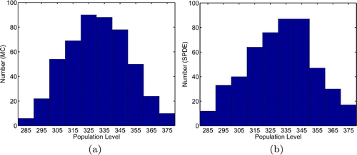
Figure 3. Calculated distribution of average size at time t = 0.5 for 500 sample paths using Monte Carlo (MC) and the SPDE (10) and (11).

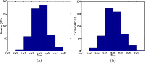
Table 5. Monte Carlo (MC) and SPDEs (10) and (11) calculational results at time t = 0.5.

Total number of individuals	Standard deviation in number of individuals	Individual average size	Standard deviation in size
330.16 (MC)	20.852 (MC)	0.25099 (MC)	0.00946 (MC)
331.46 (SPDE)	22.211 (SPDE)	0.25063 (SPDE)	0.01070 (SPDE)

The SPDEs (21) and (22) are numerically investigated in a similar way. To obtain a numerical procedure, the population is divided into K size intervals [x _k−1, x _k ], for k = 1, 2, …, K where , and J age intervals [y _j−1, y _j ] where and . Integrating Equation (21) over a size interval and over an age interval and using an explicit approximation in time t suggests the numerical procedure

for j = 2, 3, …, J and k = 1, 2, …, K with

where are independent and . Note that Equation (25) is an Euler-Maruyama 19 approximation to the system of Itô SDEs (17). In particular, in solving Equations (25) and (26), the values of u _{j, k, 0}, for , are set equal to the initial population levels. Then, Equation (25) is solved for i = 1, 2, … , j = 2, 3, …, J, and where, when j = 2, the term involving u _{1, k, i} in Equation (25) is replaced by the equivalent terms on the right-hand side of Equation (26).

Numerical solution of Equations (25) and (26) were compared with results obtained using an independent Monte Carlo computational procedure for approximating the age- and size-structured population levels. In the Monte Carlo procedure, the population was divided into 200 size-age classes and time was divided into 4000 steps where the final time was taken, for illustrative purposes, as t = 1. For each time step, each sub-population was checked for a death, birth, or size change using the probabilities given in Tables 3 and 4. To compare the two independent computational approaches, the growth rate, death rate, birth rate, and initial population were assumed to be , , , , respectively, with x _min = 0, x _max = 1, y _min = 0, and y _max = 1. For these parameters, the growth rate declines with size x and age y, the death rate increases rapidly as the maximum age y = 1 is reached, and the birth rate size distribution peaks at size x = 1/2. With these parameter selections, the exact solution to the deterministic age- and size-structured model (12) is with the total number of individuals . Thus, the deterministic population level increases exponentially with an average size of the individuals of 0.5 and with an average age of 0.25. Of interest here is the random behaviour of the population.

Summarized in Tables 6 and 7 are the results for the 500 sample paths (500 different runs) for the SPDE numerical method and for the Monte Carlo procedure. Notice that the results for the two different computational procedures are close. The population levels (total number of individuals), average individual size, and the average individual age at time t = 1 for 500 sample paths are shown in Figures 4, 5 and 6. It is clear that the SPDE accurately models the dynamics of the age- and size-structured populations.

Figure 4. Calculated distribution of populations levels at time t = 1.0 for 500 sample paths using Monte Carlo (MC) and the SPDE (21) and (22).

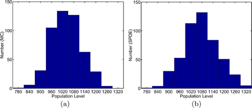
Figure 5. Calculated distribution of average size at time t = 1.0 for 500 sample paths using Monte Carlo (MC) and the SPDE (21) and (22).

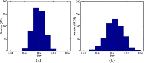
Figure 6. Calculated distribution of average age at time t = 1.0 for 500 sample paths using Monte Carlo (MC) and the SPDE (21) and (22).

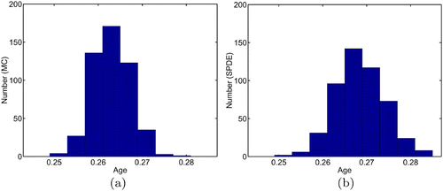
Table 6. Monte Carlo (MC) and SPDE (21) and (22) calculational results at time t = 1.0.

Total number of individuals	Standard deviation in number of individuals	Individual average size	Standard deviation in size
1038.89 (MC)	82.36 (MC)	0.49963 (MC)	0.00404 (MC)
1076.52 (SPDE)	96.53 (SPDE)	0.50180 (SPDE)	0.00599 (SPDE)

Table 7. Monte Carlo (MC) and SPDE (21) and (22) calculational results at time t = 1.0.

Individual average age	Standard deviation in age
0.26318 (MC)	0.00410 (MC)
0.26855 (SPDE)	0.00570 (SPDE)

5. Summary and conclusions

SPDEs are becoming increasingly important in applied mathematics 14–16,21. Recently developed techniques 3 6 are applied in the present investigation to derive SPDEs for age- and size-structured populations. In the derivation procedure, the deterministic and stochastic terms in the differential equation system are simultaneously derived. First, a discrete stochastic model is constructed. Next, an SDE system is derived. Finally, a particular SPDE follows from the SDE system. The SPDE for a size-structured population is given by Equations (10) and (11). The SPDE for an age- and size-structured population is given by Equations (21) and (22). The stochastic equations generalize the deterministic size- and age-structured models and include the demographic influences of randomly varying births, deaths, and size changes. Hence, random influences on certain properties of a structured population, such as on persistence time or on size variability, can be studied using these SPDEs. The SPDEs derived for age- and size-structured population models are solved numerically and compared with an independently formulated Monte Carlo method. The computational results between the two different numerical methods are in good agreement supporting the accuracy of the SPDE derivation procedure.

Acknowledgements

The author acknowledges partial support from the National Science Foundation grant NSF-DMS 0718302.

References

- Ackleh , A. S. , Deng , K. and Thibodeaux , J. J. 2007 . A monotone approximation for a size-structured population model with a generalized environment . J. Biol. Dyn. , 1 : 291 – 304 .
- Allen , E. J. 2007 . Modeling With Itô Stochastic Differential Equations , Dordrecht : Springer .
- Allen , E. J. 2008 . Derivation of stochastic partial differential equations . Stoch. Anal. Appl. , 26 : 357 – 378 .
- Allen , L. J.S. 2003 . An Introduction to Stochastic Processes with Applications to Biology , Upper Saddle River, New Jersey : Pearson Education Inc .
- Allen , L. J.S. and Allen , E. J. 2003 . A comparison of three different stochastic population models with regard to persistence time . Theor. Popul. Biol. , 68 : 439 – 449 .
- Allen , E. J. , Allen , L. J.S. , Arciniega , A. and Greenwood , P. E. 2008 . Construction of equivalent stochastic differential equation models . Stoch. Anal. Appl. , 26 : 274 – 297 .
- Allen , E. J. , Allen , L. J.S. and Schurz , H. 2005 . A comparison of persistence-time estimation for discrete and continuous stochastic population models that include demographic and environmental variability . Math. Biosci. , 196 : 14 – 38 .
- Allen , E. J. , Novosel , S. J. and Zhang , Z. 1998 . Finite element and difference approximation of some linear stochastic partial differential equations . Stoch. Stoch. Rep. , 64 : 117 – 142 .
- Arino , J. , Gouzé , J.-L. and Sciandra , A. 2002 . A discrete, size-structured model of phytoplankton growth in the chemostat . J. Math. Biol. , 45 : 313 – 336 .
- Cabaña , E. M. 1970 . The vibrating string forced by white noise . Zeitschrift für Wahrscheinlichkeitstheorie und verwandte Gebiete , 15 : 111 – 130 .
- Childs , D. Z. , Rees , M. , Rose , K. E. , Grubb , P. J. and Ellner , S. P. 2003 . Evolution of complex flowering strategies: an age- and size-structured integral projection model . Proc. Biol. Sci. , 270 : 1829 – 1838 .
- Cushing , J. M. 1992 . A size-structured model for cannibalism . Theor. Popul. Biol. , 42 : 347 – 361 .
- Cushing , J. M. 1998 . An Introduction to Structured Population Dynamics , Philadelphia : SIAM .
- Da Prato , G. and Tubaro , L. 2006 . Stochastic Partial Differential Equations and Applications – VII , Edited by: Da Prato , G. and Tubaro , L. Boca Raton, Florida : CRC Press, Taylor & Francis Group .
- Gunzburger , M. 2007 . Numerical methods for stochastic PDEs . SIAM News , 40 : 3
- Holden , H. , Øksendal , B. , Ubøe , J. and Zhang , T. 1996 . Stochastic Partial Differential Equations: A Modeling, White Noise Functional Approach , Boston, Massachusetts : Birhäuser .
- Kato , N. 2006 . Linear size-structured population models and optimal harvesting problems . Int. J. Ecol. Dev. , 5 : 6 – 19 .
- Kato , N. , Oharu , S. and Shitaoka , K. 2007 . Size-structured population models and harvesting problems . J. Comput. Appl. Math. , 204 : 114 – 123 .
- Kloeden , P. E. , Platen , E. and Schurz , H. 1994 . Numerical Solution of SDE Through Computer Experiments , Berlin : Springer .
- Kostova , T. 2003 . An explicit third-order numerical method for size-strucured population equations . Numer. Meth. Partial Diff. Equ. , 19 : 1 – 21 .
- Schurz , H. 2007 . Nonlinear stochastic wave equations in R 1 with power-law nonlinearity and additive space-time noise . Contemp. Math. , 440 : 223 – 242 .
- Sinko , J. W. and Streifer , W. 1967 . A new model for age-size structure of a population . Ecology , 48 : 910 – 918 .
- Thieme , H. R. 1991 . Analysis of age-structured population models with an additional structure . Lect. Notes Pure Appl. Math. , 131 : 115 – 126 .
- Walsh , J. B. 1986 . “ An introduction to stochastic partial differential equations ” . In Lect. Notes in Mathematics – Volume 1180 , Edited by: Dold , A. and Eckmann , B. 265 – 439 . Berlin : Springer-Verlag .
- Webb , G. F. 1985 . Theory of Age-Dependent Population Dynamics , New York : Marcel-Dekker .
![Figure 1. A Brownian Sheet on [0, 5]×[0, 5].](/cms/asset/5ec21c17-e0cd-43e2-94b2-863be9291dad/tjbd_a_316441_o_f0001g.jpg)