Dynamic equilibria in an epidemic model with voluntary vaccinations†

^†Comments and suggestions from anonymous referees of the journal are gratefully acknowledged. This paper is dedicated to the loving memory of Lucy Hauser

Abstract

The dynamics of an epidemic model with voluntary vaccinations are studied. Individual vaccination decisions are modelled using an economic/game-theoretic approach: agents in the model decide whether to vaccinate or not by weighing the cost and benefit of vaccination and choose the action that maximizes their net benefit. It is shown that, when vaccine efficacy is low, there are parameter values for which multiple steady-state equilibria and periodic equilibria coexist. When multiplicity of steady states is obtained, which one the population reaches in some cases depends entirely on agents’ expectations concerning the future course of an epidemic and not on the initial conditions of the model.

^†Comments and suggestions from anonymous referees of the journal are gratefully acknowledged. This paper is dedicated to the loving memory of Lucy Hauser

Keywords:

• voluntary vaccinations
• dynamic programming
• rational expectations
• multiple equilibria
• periodic equilibria

1. Introduction

The HIV/AIDS pandemic has already claimed the lives of over 25 million people over the last quarter century, and currently 40 million people are living with HIV 17. Although the epidemic has diminished or stabilized in some regions of the world, worldwide the number of people newly infected with HIV continues to grow, as does the number of deaths due to AIDS 15. Many experts believe that the best hope for combating the epidemic is a prophylactic vaccine 5 7 8 13, although, given the mutability of HIV, it is highly unlikely that a vaccine would provide sterilizing immunity, the ability to block infection completely 6 9.

Recently, Chen 4 introduced a mathematical model of epidemics to analyse the effect of an imperfect vaccine on the prevalence of an infectious disease such as HIV/AIDS. Unlike most of the existing literature on the modelling of infectious disease transmission, that paper focuses on the case in which vaccination is voluntary, although the impact of mandatory vaccination programmes is also considered. (Other recent papers that have studied epidemiological models with voluntary vaccinations are Bauch and Earn 1, Reluga et al. 10, and Vardavas et al. 16.) To model individuals’ decision of whether to vaccinate or not, Chen 4 utilizes an economic$/$game-theoretic approach and assumes that individuals weigh the cost and benefit of vaccination and choose the action that maximizes their net benefit. In general, this net benefit depends on the cost of the vaccine, the efficacy of the vaccine, and the prevalence of the disease. That analysis shows that, unless vaccine efficacy is sufficiently high, multiple endemic steady states that differ in vaccine coverage and disease prevalence can coexist, i.e., fixing model parameter values, if vaccine efficacy is low, then the model can have steady-state equilibria in which vaccine coverage is high and disease prevalence is low as well as steady-state equilibria in which vaccine coverage is low and as a result disease prevalence is high.

Since the analysis in Chen 4 is confined to steady states, it does not shed any light on what factors determine which steady-state equilibrium will be reached when multiple equilibria coexist. In this paper, we study the dynamics of the model in Chen 4 and focus on the following question: when multiplicity of steady states is obtained, which equilibrium does the population end up in given any initial condition? As is customary in economics, we assume that the agents in the model are forward-looking and have perfect foresight (or rational expectations) in the sense that, when they are deciding what action to take at any point in time, they consider all the possible future consequences of their action and that their estimate of the likelihood of some future event occurring is correct.1 This assumption of rational expectations is also employed in the analysis of a related epidemic model looking at the effect of behavioural changes on the prevalence of a sexually transmitted disease 3.

The analysis here reveals that, in addition to steady-state equilibria, the model can have cyclical equilibria in which vaccine coverage and hence disease prevalence oscillate periodically. It is also shown that, since agents’ vaccination decisions in the model depend on their expectations concerning future disease prevalence levels, in some cases which steady state the population ends up in when multiple steady states coexist is determined solely by agents’ beliefs regarding prevalence levels in the future and not by the initial prevalence level. Although the model presented here is highly stylized, the main purpose of the paper is to derive and elucidate some major implications of the concept of rational expectations in the context of infectious disease transmission.

The paper is organized as follows. The model is introduced in Section 2. In Section 3, we provide the main results of the analysis; specifically, we give the conditions under which there exist multiple steady-state equilibria, show that the model can also give rise to periodic equilibria, and establish the key role played by agents’ expectations in determining which steady state the population reaches when multiple steady-state equilibria coexist. Section 4 summarizes and concludes.

2. The model

Time is discrete and denoted by t=0, 1, 2, …. There is a continuum of agents, each of whom can be in one of two possible health states: susceptible and infected with an infectious disease. We assume that being infected is an absorbing state, i.e., once infection is acquired, agents remain infected for the remainder of their lives. Let p _t ∈[0, 1] denote the proportion of agents who are infected at the beginning of period t.

To specify the welfare of the agents, let u _i denote the per-period utility (or payoff) from being infected, and let u _s be the per-period utility from being in the susceptible state, where . The utility at death is 0. Suppose a vaccine for the disease exists and, in any period, susceptible agents can choose to be vaccinated at a utility cost of c>0, i.e., if a susceptible agent chooses to vaccinate in some period, then the agent's net utility in that period is u _s −c. To keep things simple, it is assumed that this vaccination cost c is identical for all susceptible agents.2 Vaccination reduces the transmission probability of the disease (the probability of acquiring an infection conditional on contacting an infective): an unvaccinated susceptible agent becomes infected with probability β∈(0, 1] after contacting an infected agent, while the corresponding probability for a vaccinated susceptible agent is , where denotes the efficacy of the vaccine. The vaccine confers lifelong immunity, which means that an agent will choose to be vaccinated at most once.

For convenience, we assume that an agent's life span is independent of the agent's health state: in any period, an agent, whether infected or not, dies at the end of the period with probability δ∈(0, 1]. Note that, with a continuum of agents, δ is also the fraction of agents who die in every period. Upon death, an agent is immediately replaced by an unvaccinated susceptible agent so that the total population size remains constant over time.

In every period, all agents, infected or not, make one contact with another randomly chosen agent so that there is proportional mixing in the population. This implies that an unvaccinated susceptible agent in period t has probability β p _t of becoming infected during that period, while the probability of acquiring an infection during the same period is for a susceptible agent who has been vaccinated.

Susceptible agents are forward-looking and seek to maximize the expected value of their lifetime utility by choosing when, if ever, to be vaccinated. We can use the technique of dynamic programming to solve a susceptible agent's optimization problem 11 14. Given the sequence of disease prevalence levels , the expected lifetime utility for a vaccinated susceptible agent starting in period t, , satisfies the following equation:

The optimality equation for an unvaccinated susceptible agent in period t is

where is the expected lifetime utility starting from period t for an unvaccinated susceptible agent who behaves optimally. The first term in the maximand is the expected lifetime utility from period t onwards if the agent chooses not to be vaccinated in period t, while the second term in the maximand is the expected lifetime utility starting from period t if the agent is vaccinated in period t. Letting , , and , we can rewrite Equations (1) and (2), respectively, as follows:

and

Note that the Contraction Mapping Theorem ensures that there exists uniquely a pair of value functions U and W that satisfy Equations (3) and (4).

Given susceptible agents’ vaccination decision, we can derive a system of equations describing how the prevalence of the disease behaves over time. Letting v _t ∈[0, 1] and s _t ∈[0, 1], respectively, denote the proportion of vaccinated and unvaccinated susceptible agents at the beginning of period t, we have

where ∀ t and is the fraction of unvaccinated susceptible agents in period t who choose to be vaccinated in that period. It is easy to check that, given p ₀∈[0, 1], s ₀∈[0, 1], and v ₀∈[0, 1], Equations (5)–(7) imply that p _t ∈[0, 1], s _t ∈[0, 1], and v _t ∈[0, 1] ∀ t. Notice that, given the value functions U and W satisfying Equations (3) and (4), α _t is defined by

Given the derivations above, we can define an equilibrium of the model as follows.

Definition 1

Given p ₀∈[0, 1], s ₀∈[0, 1], and v ₀∈[0, 1] such that , the sequence is a rational expectations equilibrium (REE) if: (i) given , , , and satisfy Equations (5)–(7) ∀ t; and (ii)given , satisfies Equation (8) ∀ t.

Note that, in this model, unvaccinated susceptible agents’ behaviour in every period depends on current and future prevalence levels, which in turn are determined by the agents’ vaccination decisions. The concept of an REE is simply the requirement that agents’ behaviour and the prevalence of the disease be consistent with one another.

3. Results

3.1. Steady-state REE

We begin our analysis by looking at steady-state REEs (SSREEs) in which , p _t =p, s _t =s, and v _t =v ∀ t. We say that a steady state is endemic if p>0. By Equations (5)–(7), in a steady state, p, s, and v solve

In addition, Equations (3) and (4), respectively, yield

and

Proposition 1, the proof of which is given in Chen 4, shows the conditions under which an endemic SSREE exists and is unique.

Proposition 1

An endemic SSREE exists if . Moreover, it is unique if .

Henceforth, it will be assumed that . Although the condition guarantees uniqueness of an endemic equilibrium, it is not necessary. The result below gives the conditions under which multiple SSREEs can coexist. To state the result, let us define and . It can be easily verified using Equations (9)–(11) that p is the steady-state prevalence level when α=1 and is the prevalence level in a steady state if no susceptible agent chooses to vaccinate, i.e., α=0.

Proposition 2

If and

then multiple SSREEs coexist.

To see this, let , which can be thought of as the benefit of vaccination, since B(p) is the increase in expected lifetime utility in a stead state from having being vaccinated. By Equations (8), (12), and (13), we have

It is easy to show that as so that, given any such that p<p′, we can have , i.e., if , then it is possible for agents to choose not to vaccinate at high prevalence levels even though they would choose to vaccinate at some lower prevalence levels. Now, α=1 implies by Equations (9)–(11) that , so from Equation (14) an {all-vaccinate} SSREE with exists if . On the other hand, α=0 gives using Equations (9)–(11), therefore, Equation (14) tells us that a {no-vaccination} SSREE with exists if . Since implies that can be smaller than , multiple SSREEs coexist when . If , there also exists a ‘mixed strategy’ SSREE in which α∈(0, 1) and the prevalence p satisfies B(p)=c. Let p* denote the steady-state prevalence level in this equilibrium. Note that, given , it must be the case that . Since the benefit of vaccination equals its cost in this steady-state equilibrium, agents are indifferent between choosing to vaccinate and choosing not to. Therefore, it is consistent with rational behaviour for some agents to get vaccinated and for others not to. Note that if c falls outside the region given in Proposition 2, then an SSREE need not be unique. Specifically, if , then the all-vaccinate steady state with is the unique SSREE, and if , then the no-vaccination steady state with is an SSREE but not necessarily the only one.

For an example of the coexistence of multiple SSREEs, suppose β=1, δ=0.07, , u=100, and c=338. In this case, , , and (93p+35)). Figure 1 shows how B(p) compares to the cost of vaccination c as p is varied between 0 and 1. As can be seen from Figure 1, an SSREE with exists since B(0.92)<c, and an SSREE with exists given that B(0.62)>c. There is also a third SSREE in which .

To see why the condition guarantees uniqueness of an SSREE, note that B(p) is monotonically increasing in p (in the unit interval [0, 1] ) when the given condition holds. This means that the benefit of vaccination will always rise as the prevalence increases so that, by Equation (14), the proportion of agents who choose to vaccinate in any period is increasing in p. At the same time, it is easy to show using Equations (9)–(11) that the steady-state prevalence is decreasing in α, the steady-state proportion of agents who choose to vaccinate. Now, if p ₁ and p ₂, where p ₂>p ₁, are both equilibrium steady-state prevalence levels, then, assuming , the proportion of agents who choose to vaccinate must be higher given p ₂. However, Equations (9)–(11) tell us that if the proportion of agents who vaccinate is greater given p ₂, then p ₂ must be lower than p ₁, a contradiction. Therefore, when , multiple steady-state equilibria cannot coexist.

Figure 1. The benefit and cost of vaccination as functions of the steady-state prevalence. The parameter values used are: β=1, δ=0.07, ϵ=0.8, u=100, and c=338. With the given parameter values, and p=0.62. The solutions to the equation B(p)=c are 0.78 and 0.036. Since there does not exist a solution to Equations (9)–(11) satisfying p=0.036 and α∈[0, 1], there cannot be an SSREE in which p=0.036. On the other hand, we obtain α=0.48∈[0, 1] from solving Equations (9)–(11) given p=0.78. Therefore there exists an SSREE with (α, p)=(0.48, 0.78).

3.2. Convergence to steady state

When multiple endemic SSREEs coexist, what determines which steady state will be reached and what is the role played by the initial conditions, i.e., p ₀, v ₀, and s ₀? For this subsection, we will assume that v ₀=0 (this captures the situation in which the vaccine is first introduced at time 0) so that the initial condition of the model is determined solely by p ₀.

Suppose the model parameter values are such that an all-vaccinate SSREE with and a no-vaccination SSREE with both exist. By Proposition 1, this means that . Given the initial prevalence level p ₀>0, let us consider the following questions: can there be an REE\ in which α _t =0 ∀ t? Can there be an REE in which α _t =1 ∀ t? Let us look at these two cases separately.

3.2.1. REE with α _t =0 ∀ t

Given p ₀, suppose α _t =0 ∀ t. By Equations (5)–(7), this along with the assumption that v ₀=0 imply that

Therefore, given p ₀ and Equation (15), we have a sequence of disease prevalence , where . Let and , respectively, denote the value functions W and U given and this sequence . Condition (8) tells us that is optimal if

where and , respectively, satisfy

and

Note that if condition (16) is satisfied, then there is an REE with that converges to the no-vaccination SSREE\ in which .

3.2.2. REE with α _t =1 ∀ t

Given p ₀, suppose α _t =1 ∀ t. Using Equations (5)–(7), this and v ₀=0 imply that

which defines a sequence of prevalence given p ₀, with . Let W and U, respectively, denote the value functions W and U given α _t =1 ∀ t and this sequence . Condition (8) tells us that α _t =1 ∀ t is optimal if

where U and W, respectively, satisfy

and

Therefore, an REE with α _t =1 ∀ t exists if condition (20) holds, and this REE converges to the all-vaccinate SSREE in which .

To establish whether REEs of the types described above exist given p ₀, we used the Method of Successive Approximation from dynamic programming 11 14 to find the functions , , U, and W in order to check whether condition (16) or (20) holds (see Appendix A). The main result of the analysis is that, fixing parameter values and the initial prevalence p ₀, it is possible for both REEs to exist so that the population can reach either a steady state with no vaccination or a steady state in which all susceptible agents choose to vaccinate. Put differently, there are cases in which knowing the model parameter values and the initial prevalence level p ₀ does not help us in determining which steady-state equilibrium the population will end up in.

Result 1

Given β, δ, ϵ, u, and c, there exists p ₀ for which an REE with α _t =1 ∀ t and an REE with α _t =0 ∀ t both exist.

To see this, let us consider the following specification of parameter values: β=1, δ=0.07, , u=100, and c=338. The numerical solution of the model (see Appendix A) shows that for any p ₀∈(0, 1] there is an REE with α _t =0 ∀ t, while an REE with α _t =1 ∀ t exists for all . 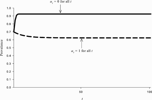This means that, starting with any prevalence level between 0.0513 and 0.973, there is an REE in which no one ever chooses to be vaccinated and the disease prevalence converges to the steady-state value , and there also exists an REE in which all susceptible agents choose to be vaccinated and the disease prevalence converges to the lower steady-state value p. An example of this is shown in Figure 2.

Figure 2. The coexistence of multiple REEs starting with the same initial prevalence level. The parameter values used are: β=1, δ=0.07, ϵ=0.8, u=100, and c=338. Given initial prevalence p ₀=0.7 (and v ₀=0), there exists an REE in which α _t =0 ∀ t and p _t converges to ; there also exists an REE in which α _t =1 ∀ t and p _t converges to p=0.62.

Just exactly what accounts for the finding that there are initial prevalence levels for which there exist an REE with α _t =1 ∀ t as well as an REE with α _t =0 ∀ t? Intuitively, the driving force behind this result is the fact that, when vaccine efficacy is low (so that ), the availability of the vaccine creates a positive feedback loop. To see this, recall that B(p), the benefit of vaccination, is decreasing in p for p above some threshold when . This means that, given a low-efficacy vaccine, if agents expect future prevalence to be sufficiently high, then they would actually have little incentive to vaccinate. However, prevalence is inversely related to the proportion of agents who choose to vaccinate. Therefore, the fewer the number of agents who vaccinate, the higher the future prevalence, which in turn further reduces the number of susceptible agents who vaccinate. Thus, the expectation that prevalence levels in the future will be high can be self-fulfilling and lead to an equilibrium in which few agents choose to vaccinate and the prevalence is high. On the other hand, if agents expect future prevalence levels to be ‘moderate’ so that vaccination is cost-beneficial,3 then this would result in lower prevalence levels in the future (although the efficacy of the vaccine places a limit on how much prevalence can be lowered). This in turn can reinforce agents’ decision to vaccinate, thus creating a positive feedback effect leading to high vaccine coverage. The self-fulfilling nature of agents’ expectations given a low-efficacy vaccine thus implies that, in certain cases, which steady state the population will end up in depends entirely on the agents’ beliefs concerning how prevalent the disease will be in the future and not on the current prevalence level.

3.3. Equilibrium switching and periodic REE

As we have seen in the previous subsection, there exist parameter values for the model such that, given an initial prevalence level p ₀ and depending on agents’ expectations concerning future prevalence levels, the population can reach either a steady state in which all susceptible agents choose to be vaccinated or one in which no one chooses to be vaccinated. Obviously, which steady state is reached has enormous welfare implications for the population, since the prevalence is lower in the steady state in which all susceptible agents are vaccinated ().

However, another implication of the model here is that, when multiple SSREEs coexist, even if the population reaches the no-vaccination steady state, the community need not be stuck there indefinitely. More specifically, if the population is at the no-vaccination steady state, then, without any exogenous shocks or external interventions, it is possible for the population to leave that steady state and reach the all-vaccinate steady state in which prevalence is lower. Put differently, there can exist an REE in which the population switches from the no-vaccination steady state to the all-vaccinate steady state (Figure 3).

Figure 3. Assuming the population is initially at the no-vaccination steady state, there can exist an REE in which susceptible agents’ behaviour changes starting at time T and the population eventually reaches the all-vaccinate steady state.

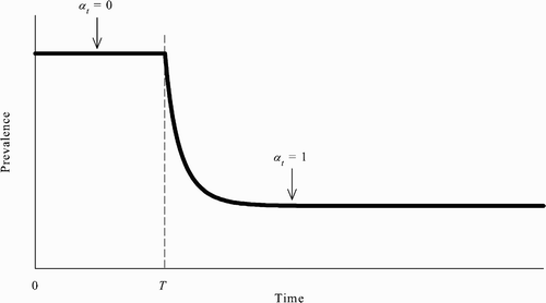
To see this, suppose that the population is at the no-vaccination steady state from time 0 to some time T−1 and that all unvaccinated susceptible agents change their behaviour at time T: all unvaccinated susceptible agents choose to be vaccinated in every period starting at time T. Formally, this assumption can be written as follows:

Note that, using Equations (5)–(7), (23)–(25) yield

We have , , and . Therefore, the population, which is at the no-vaccination steady state up until time T−1, eventually reaches the all-vaccinate steady state after the change in behaviour at time T. We now show that there exist parameter values for the model such that the situation described above (by Equations (23)–(28)) is an REE for any T.

Result 2

There exist parameter values for the model such that the sequence satisfying Equations (23)–(28) is an REE for any T.

Let and , respectively, denote the value functions W and U given Equations (23)–(28). Consider the following specification of parameter values: β=1, δ=0.07, , u=100, and c=338.

Case 1

t≥T. We already know from Section 3.2 that, given these parameter values, there exists an REE in which and α _t =1 ∀ t, i.e., α _t =1 ∀ t is a rational response by unvaccinated susceptible agents given . In this REE, and , where W and U are defined in Section 3.2. Therefore, must be optimal for unvaccinated susceptible agents given , and must be equal to , and must be equal to .

Case 2

t<T. Given that and , we have

and

which give

and

respectively. Now, according to Equation (8), is optimal for unvaccinated susceptible agents if

or, equivalently,

where and are given by Equations (29) and (30), respectively. For the given parameter values, condition (31) is satisfied for any choice of T and t<T (see Figure 4). Therefore, fixing any T, it is optimal for unvaccinated susceptible agents to choose .

Figure 4. The net cost of vaccination at time t<T given and α _t =1 ∀ t≥T. The plot shows U*(p _t )−(W*(p _t )−c), t<T, where W* and U*, respectively, satisfy Equations (29) and (30), as a function of T−t. The parameter values used are: β=1, δ=0.07, ϵ=0.8, u=100, and c=338.

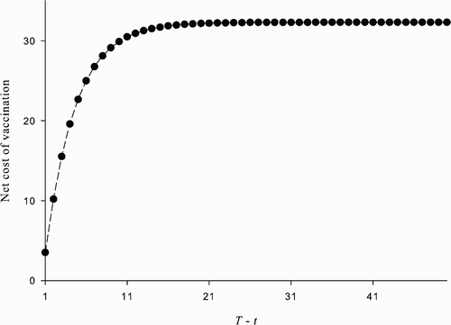
Intuitively, why such an REE exists is due to the self-fulfilling nature of agents’ expectations when vaccine efficacy is low: assuming that the population is at the no-vaccination steady state, if unvaccinated susceptible agents expect all other unvaccinated agents to switch behaviour and get vaccinated starting at some future date T (thereby driving down prevalence in the future), then, under the right conditions, it would be optimal for the agents to follow suit and choose to be vaccinated at time T. Thus, the expectation that agents would alter their behaviour in the future is self-fulfilling and results in the population moving from the no-vaccination steady state to the all-vaccinate steady state.

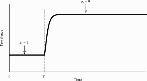
Not only are there parameter values such that there exists an REE in which the population switches from the no-vaccination steady state to the all-vaccinate steady state, given these same parameter values there can also exist an REE in which the population moves from the all-vaccinate steady state to the no-vaccination steady state. Assuming the population is initially at the all-vaccinate steady state, in this REE, the expectation that no susceptible agent would choose to get vaccinated starting at some future date T leads unvaccinated susceptible agents to optimally choose not to be vaccinated from period T onwards and results in the population moving to the no-vaccination steady state (Figure 5). To see this mathematically, suppose that the population is at the all-vaccinate steady state from time 0 to some time T−1 and that, starting at time T, all unvaccinated susceptible agents choose not to be vaccinated in every period, i.e.,

Using Equations (5)–(7), Equations (32)–(34) give

Note that , , and so that the population eventually reaches the no-vaccination steady state starting from the all-vaccinate steady state.

Figure 5. Assuming the population is initially at the all-vaccinate steady state, there can exist an REE in which susceptible agents’ behaviour changes starting at time T and the population eventually reaches the no-vaccination steady state.

Result 3

There exist parameter values for the model such that the sequence satisfying Equations (32)–(37) is an REE for any T.

Let and , respectively, denote the value functions W and U given Equations (32)–(37). Consider again the following specification of parameter values: β=1, δ=0.07, , u=100, and c=338.

Case 3

t≥T. To show that it is optimal for unvaccinated susceptible agents to choose α _t =0 , consider the following situation: and . Let and , respectively, denote the value functions W and U in this case. It can be shown that with and the given parameter specification, there exists an REE with α _t =0 ∀ t, where and (see Appendix B for details). In other words, with the given specification of parameter values, α _t =0 ∀ t is optimal for unvaccinated susceptible agents when . This implies that α _t =0 must be optimal for unvaccinated susceptible agents if and that and .

Case 4

t<T. Given the assumptions that and α _t =1 ∀ t<T, we have

and

Note that Equation (38) implies that

By Equation (8), is optimal for unvaccinated susceptible agents if

or, equivalently,

Given and , it is easy to check that the second part of condition (40) is satisfied. Moreover, the first part of condition (40) holds for any T and t<T (see Figure 6). Therefore, α _t =1 ∀ t<T is an optimal choice for unvaccinated susceptible agents for any T.

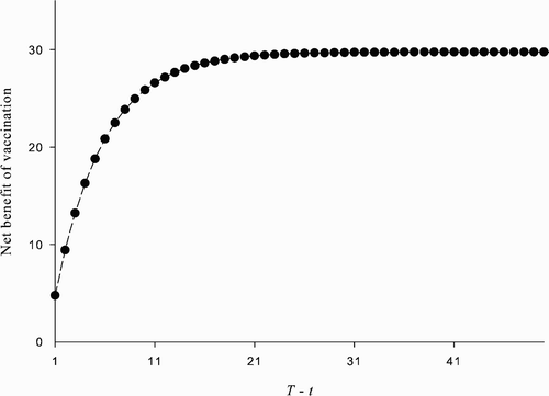
Figure 6. The net benefit of vaccination at time t<T given p _t =p ∀ t≤T and α _t =0 ∀ t≥T. The plot shows , t<T, where satisfies Equation (39), as a function of T−t. The parameter values used are: β=1, δ=0.07, ϵ=0.8, u=100, and c=338.

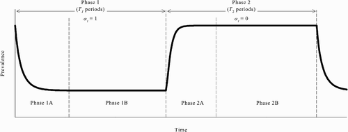
As the previous analysis shows, there are parameter values for the model such that there is an equilibrium in which the population switches from the no-vaccination steady state to the all-vaccinate steady state and an equilibrium in which the population moves in the other direction — from the all-vaccinate steady state to the no-vaccination steady state. In fact, when this situation is obtained, it is also the case that there exist periodic REEs in which the prevalence oscillates between a level arbitrarily close to and a lower level arbitrarily close to p. Since there are REEs in which the population switches from one steady state to another, we can construct a periodic REE by simply ‘piecing together’ these switches.4 More specifically, consider a cycle of period T ₁+T ₂ consisting of two phases. In the first phase (Phase 1), which lasts for T ₁ periods, all unvaccinated susceptible agents choose to be vaccinated in every period. In the second phase (Phase 2), which lasts for T ₂ periods, all unvaccinated susceptible agents choose not to be vaccinated in every period. Note that when T ₁ and T ₂ are large, the population is arbitrarily close to the all-vaccinate steady state at the end of Phase 1 and arbitrarily close to the no-vaccination steady state at the end of Phase 2. Results 2 and 3 imply that, for T ₁ and T ₂ large, there exist parameter values for the model such that the periodic behaviour described is an REE.

Intuitively, this can be seen as follows with the aid of Figure 7, which shows the time path of disease prevalence given the stated periodic behaviour. Assume that the parameter values are such that there exist REEs in which the population switches from the no-vaccination steady state to the all-vaccinate steady state (none-to-all REEs) and from the all-vaccinate steady state to the no-vaccination steady state (all-to-none REEs). Consider first Phase 1A, the early part of Phase 1 in which the prevalence is not yet close to p. Notice that, for T ₁ large, the decision problem facing an unvaccinated susceptible agent in Phase 1A is virtually identical to that such an agent faces in a none-to-all REE after the switch takes place. Since an unvaccinated susceptible agent optimally chooses to be vaccinated after the switch occurs in a none-to-all REE, it must be optimal for such an agent to choose to be vaccinated in Phase 1A given T ₁ large.

Figure 7. The existence of periodic REEs.

For T ₁ large, the disease prevalence is arbitrarily close to in Phase 1B. If T ₂ is also large, then the decision problem of an unvaccinated susceptible agent in Phase 1B is virtually the same as that such an agent faces in an all-to-none REE before the switch takes place. Because it is optimal for an unvaccinated susceptible agent to choose to be vaccinated in an all-to-none REE before the switch occurs, it must be optimal for such an agent to choose to be vaccinated in Phase 1B for large T ₂. Therefore, we can conclude that, for T ₁ and T ₂ large, choosing to be vaccinated in Phase 1 is an optimal response by unvaccinated susceptible agents.

Using arguments analogous to those above, we can argue that it is optimal for unvaccinated susceptible agents to choose not to be vaccinated in Phase 2 if T ₁ and T ₂ are both large. In Phase 2A, when the prevalence is not close to , the decision problem facing an unvaccinated susceptible agent for large T ₂ is virtually identical to that such an agent faces in an all-to-none REE after the switch occurs. Since an unvaccinated susceptible agent optimally chooses not to be vaccinated after the switch occurs in an all-to-none REE, it must be optimal for such an agent to choose not to be vaccinated in Phase 2A for large T ₂.

Finally, consider Phase 2B, in which the prevalence is arbitrarily close to for T ₂ large. If T ₁ is also large, then the decision problem of an unvaccinated susceptible agent in Phase 2B is virtually the same as that such an agent faces in a none-to-all REE before the switch takes place. Because it is optimal for an unvaccinated susceptible agent to choose not to be vaccinated in a none-to-all REE before the switch occurs, it must be optimal for such an agent to choose not to be vaccinated in Phase 2B for large T ₁. Therefore, we can conclude that, for T ₁ and T ₂ large, choosing not to be vaccinated in Phase 2 is an optimal response by unvaccinated susceptible agents.

Note that the existence of periodic REEs for T ₁ and T ₂ large is not due to the assumption that time is discrete in the model. Since the coexistence of multiple SSREEs or the technique for proving the existence of periodic equilibria described above does not depend on whether the model is formulated in discrete or continuous time, the result that there are parameter values for which periodic REEs exist when the period of cycles is sufficiently large should also obtain in the continuous-time version of the model.

4. Conclusion

In this paper, we have shown that, with rational, forward-looking agents, the impact of an imperfect vaccine when vaccination is voluntary on the prevalence of an infectious disease can depend critically on the agents’ expectations concerning the future course of an epidemic. In particular, when vaccine efficacy is low, multiple steady-state equilibria can coexist and, in certain cases, which steady state is reached depends entirely on agents’ expectations and not on the initial conditions of the model. The finding that expectations can affect the equilibrium vaccine coverage and disease prevalence has obvious policy implications and suggests that the ability of the government and public health authorities to alter or shape people's beliefs concerning the impact of a vaccine on future prevalence can be vital in determining how many people choose to be vaccinated.

Although, for the sake of simplicity, we have assumed in this paper that all susceptible agents have the same cost of vaccination, the same qualitative results should obtain if agents are heterogeneous and differ in their preferences for vaccination. Similarly, dropping the assumption that susceptible and infected agents face the same probability of death at the end of each period would not substantively alter the results of the analysis. To see why, note that an unvaccinated susceptible agent's decision problem would essentially remain unchanged if the assumption that infected agents face a higher probability of death were employed instead. Suppose in any period a susceptible agent and an infected agent die at the end of the period with probabilities δ and δ _i , respectively, where . Given this, Equations (1) and (2), respectively, yield

and

Now, letting , , and , Equations (41) and (42) can be rewritten as Equations (3) and (4), respectively. Therefore, the maximization problem facing unvaccinated susceptible agents and, hence, their behaviour do not depend on whether δ _i is equal to or higher than δ. Although assuming that would necessitate some slight modifications to Equations (5)–(7), it would not alter the implication that the steady-state prevalence is decreasing in the proportion of susceptible agents who choose to be vaccinated. Consequently, none of the results given here would be affected substantively by dropping the restriction that and assuming that instead.

As we have shown here, the dynamical behaviour of the model is rich and complex. Future work in this area can continue to characterize the set of equilibria of the model. Other research projects can analyse variations of the model and consider, for instance, the effects of heterogeneity in transmission probability, waning immunity, and policy changes that affect the accessibility of the vaccine.

Notes

^†Comments and suggestions from anonymous referees of the journal are gratefully acknowledged. This paper is dedicated to the loving memory of Lucy Hauser

For a technical exposition of rational expectations in the context of dynamic macroeconomic models, see e.g. Sargent 12.

The steady-state analysis in Chen 4 allows for heterogeneity in this cost c.

Vaccination cannot be optimal when prevalence is sufficiently low.

This technique of establishing the existence of a periodic REE is the same one employed by Burdett and Coles 2 to prove the existence of a periodic equilibrium with rational expectations in an economic model of the marriage market.

Appendix A

We show how to numerically solve the model and determine whether an REE with α _t =0 ∀ t or α _t =1 ∀ t exists.

REE with α _t =0 ∀ t

Since if (and v ₀=0), Equations (17) and (18) tell us that and , respectively, are the solutions to the functional equations

and

Now, α _t =0 ∀ t is indeed optimal if condition (16) holds. Notice that, using Equations (17) and (18), condition (16) can be rewritten as

To numerically solve for the functions and , we employed the following iterative procedure (Method of Successive Approximation):

1. Start with the functions and ;

2. Given functions and for some integer n, define the functions and , respectively, by

   and

Equations (46) and (47) define the sequences and , respectively, and the Contraction Mapping Theorem tells us that and . In particular, it is easy to show that and under the sup norm so that the functions and obtained using this procedure can be made arbitrarily close to and , respectively, by choosing n sufficiently large.

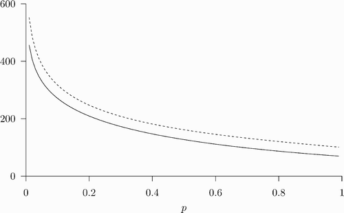
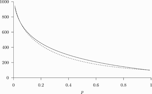
We chose n to be the first integer m such that and . To determine whether condition (45) holds for all p _t in the sequence defined using the equation , with p ₀ given, we verified whether the condition is satisfied for all p _t in the sequence . We concluded that, given p ₀, an REE with α _t =0 ∀ t exists if for all p _t in . Figure 8 shows a plot of and with respect to p for the example in Section 3.2. Since , an REE with exists .

Figure 8. A plot of (solid line) and (dashed line) with respect to p, where and , respectively, solve Equations (43) and (44). The parameter values used are: β=1, δ=0.07, ϵ=0.8, u=100, and c=338.

REE with α _t =1 ∀ t

Note that, given p ₀, α _t =1 ∀ t implies that the sequence of prevalence satisfies Equation (19). For convenience, let . Now, choosing α _t =1 ∀ t is indeed optimal if Equation (20) holds. Using Equations (21) and (22), Equation (20) can be rewritten as

where W solves the functional equation

and U satisfies

To numerically solve for the function W, we employed the following iterative procedure (Method of Successive Approximation):

1. Start with the function , where ;

2. Given the function for some integer n, define the function by

Equation (51) defines the sequence , and the Contraction Mapping Theorem tells us that , with under the sup norm. Therefore, the function obtained using this procedure can be made arbitrarily close to W by choosing n sufficiently large.

We chose n to be the first integer m such that and concluded that, given p ₀, an REE with exists if

where , for all p _t in the sequence which is defined inductively by . Figure 9 shows a plot of and with respect to p for the example discussed in Section 3.2. Since Equation (52) holds for the parameter values used as long as , and since if and α _t =1 ∀ t, an REE with exists for all .

Figure 9. A plot of W (p)−c (solid line) and u+(1−δ) (1−β p) U (f(p)) (dashed line) with respect to p, where W solves Equation (49) and U satisfies Equation (50). The parameter values used are: β=1, δ=0.07, ϵ=0.8, u=100, and c=338. The two curves cross when p=0.0513 and p=0.973.

Appendix B

If , then Equations (5) and (6) yield

where we have substituted 1−s _t −p _t for v _t . For convenience, define the following:

To see if an REE with α _t =0 ∀ t and exists given β=1, δ=0.07, , u=100, and c=338, we first solved the functional equations

using the Method of Successive Approximation (described in Appendix A). Having obtained the functions W* * and U* *, condition (8) implies that α _t =0 is indeed an optimal choice for unvaccinated susceptible agents at time t if . The unshaded region in Figure 10 is the set of (p, s) at which , while the shaded region is the set of (p, s) at which . The point is indicated by the black dot in Figure 10. Given the initial condition , every point (p _t , s _t ) in the sequence defined using Equations (53) and (54) lies on the dashed line in the figure. Since the dashed line lies entirely in the unshaded region, we can conclude that there exists an REE with α _t =0 ∀ t given . The value functions and mentioned in the text are defined as follows: given s ₀=δ; given s ₀=δ.

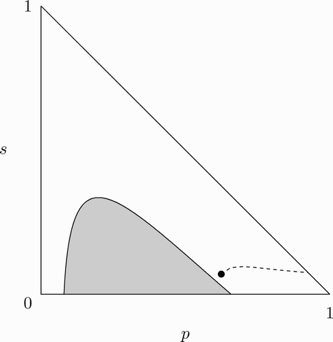
Figure 10. A comparison of U* *(p, s) and W* *(p, s)−c. The set of (p, s) such that U* *(p, s)>W* *(p, s)−c is indicated by the unshaded region, while the shaded region is the set of (p, s) at which U* *(p, s)≤W* *(p, s)−c. The point (p, s)=(p, δ) is indicated by the black dot. The parameter values used are: β=1, δ=0.07, ϵ=0.8, u=100, and c=338.

References

- Bauch , C. and Earn , D. 2004 . Vaccination and the theory of games . Proc. Nat. Acad. Sci. , 101 : 13391 – 13394 .
- Burdett , K. and Coles , M. 1998 . Separation cycles . J. Econom. Dynam. Control , 22 : 1069 – 1090 .
- Chen , F. 2004 . Rational behavioral response and the transmission of STDs . Theoret. Popul. Biol. , 66 : 307 – 316 .
- Chen , F. 2006 . A susceptible-infected epidemic model with voluntary vaccinations . J. Math. Biol. , 53 : 253 – 272 .
- Esparza , J. 2001 . An HIV vaccine: how and when? . Bull. World Health Organ. , 79 : 1133 – 1137 .
- Hanke , T. 2001 . Prospect of a prophylactic vaccine for HIV . Br. Med. Bull. , 58 : 205 – 218 .
- Johnston , M. and Flores , J. 2001 . Progress in HIV vaccine development . Curr. Opin. Pharmacol. , 1 : 504 – 510 .
- Letvin , N. 2005 . Progress toward an HIV vaccine . Ann. Rev. Med. , 56 : 213 – 223 .
- Levy , J. 2001 . What can be achieved with an HIV vaccine? . Lancet , 357 : 223 – 224 .
- Reluga , T. , Bauch , C. and Galvani , A. 2006 . Evolving public perceptions and stability in vaccine uptake . Math. Biosci. , 204 : 185 – 198 .
- Ross , S. 1983 . Introduction to Stochastic Dynamic Programming , New York, NY : Academic Press .
- Sargent , T. 1987 . Macroeconomic Theory , 2 , San Diego, CA : Academic Press . Inc
- Spearman , P. 2003 . HIV vaccine development: lessons from the past and promise for the future . Curr. HIV Res. , 1 : 101 – 120 .
- Stokey , N. and Lucas , R. 1989 . Recursive Methods in Economic Dynamics , Cambridge, MA : Harvard University Press . (with E. Prescott)
- UNAIDS/WHO . 2006 . AIDS Epidemic Update: 2006 , Geneva, , Switzerland : UNAIDS/WHO .
- Vardavas , R. , Breban , R. and Blower , S. 2007 . Can influenza epidemics be prevented by voluntary vaccination? . PLoS Comput. Biol. , 3 : 0001 – 0007 .
- WHO . 2006 . Towards Universal Access by 2010 , Geneva, , Switzerland : WHO .