Pattern formation in prey-taxis systems

Abstract

In this paper, we consider spatial predator–prey models with diffusion and prey-taxis. We investigate necessary conditions for pattern formation using a variety of non-linear functional responses, linear and non-linear predator death terms, linear and non-linear prey-taxis sensitivities, and logistic growth or growth with an Allee effect for the prey. We identify combinations of the above non-linearities that lead to spatial pattern formation and we give numerical examples. It turns out that prey-taxis stabilizes the system and for large prey-taxis sensitivity we do not observe pattern formation. We also study and find necessary conditions for global stability for a type I functional response, logistic growth for the prey, non-linear predator death terms, and non-linear prey-taxis sensitivity.

Keywords:

• predator–prey models
• prey-taxis
• stability
• pattern formation
• biological control

AMS Subject Classification :

• 92C15
• 92D25
• 92D40
• 34D23

1. Introduction

There are basically three mechanisms for spatial pattern formation in systems of two reaction–advection–diffusion equations; the Turing patterns 25, chemotaxis patterns 12, and patterns created through reaction kinetics, e.g. the Brusselator 15. Turing patterns typically arise for a fast inhibitor and a slow activator. Chemotaxis patterns are based upon aggregation towards a chemical signal.

For a predator–prey system without prey-taxis, Okubo and Levin 26 note that an Allee effect in the functional response and a density-dependent death rate of the predator are necessary to generate spatial patterns. The inclusion of species migration (constant flow) as an additional transport process may also increase the possibility of pattern formation 13. The directional movement of zooplankton plays a role in generating patterns in a plankton community model 22. For the same system, diffusion also generates pattern formation, and the combined effects of diffusion and velocity result in spatial pattern and an instability like travelling waves, i.e. travelling patchy distributions 23. Indeed, the magnitude of the relative flow velocity determines the flow-induced instability 28. Various travelling wave solutions have been studied with similar systems 4 18 33. In particular, 4 33 also considered escaping behaviours of prey from predation.

For chemotaxis models, spatial patterns have been studied analytically and numerically (see, for example, 7 35 36). In contrast to the rich development of chemotaxis models, the pattern formation of prey-taxis models is still open to wide investigations. Lewis 20 studied pattern formation in plant and herbivore dynamics and herbivory-taxis was seen to reduce the likelihood of pattern formation. Arditi et al. 3 and Chakraborty et al. 6 considered a different aspect of predator response to the prey distribution that the velocity of the predators is dependent on prey density.

The goal of this paper is to investigate the contribution of predator and prey movements to spatial pattern formation in predator–prey systems. In particular, we consider foraging behaviour of predators that move towards high prey density. For that, we extend the predator–prey diffusion–reaction model in 27 by incorporating the concept of prey-taxis 14.

1.1. The model

A prey-taxis model was derived by Kareiva and Odell in 14, and they studied predator aggregation in high prey density areas. Later the model was applied to estimate the mean travel time of a predator to reach a prey resource 9. Here we extend the Kareiva and Odell model to studying pattern formation.

The prey-taxis model discussed below contains both diffusion terms that might lead to Turing-type instabilities and a prey-taxis term that might lead to aggregation of predators on local concentrations of prey. In this paper, we will investigate the relative importance of these effects for spatial pattern formation. Prey-taxis allows predators to search more actively for prey, and can generate different spatial patterns from those formed in models without prey-taxis. Generally speaking, we find that prey-taxis tends to stabilize the predator–prey interactions.

The characteristic feature of prey-taxis equations is that taxis is incorporated as an advection term 14 17. In this paper, we consider the following prey-taxis model

where ε and γ are positive dimensionless parameters. Here v(x, t) and n(x, t) are prey density and predator density, respectively. f(v) is the per capita prey population growth rate, h(v, n) is the functional response, and is the mortality rate of the predator without the prey. The prey sensitivity, χ(v), is a non-negative non-increasing function of the prey density, and as example, we choose , or .

To investigate the pattern formation properties of Equations (1) and (2), we first consider (1) and (2) without taxis, i.e. χ=0. Secondly, we study the full model (1) and (2) with χ≠0. In Section 2.1, we study pattern formation for Equations (1) and (2). It turns out that pattern formation crucially depends on the functional forms of functional response h(v, n), on the death rate δ (n), and on the prey growth kinetics f(v). We investigate typical cases, that are discussed in the literature, see, e.g. 34. For h(v, n) we consider type I (linear) functional response h(v, n)=v, type II (hyperbolic) functional response , linear-ratio functional response , and hyperbolic-ratio functional response . The death rate δ(n) is either constant or density-dependent . For the prey kinetics, we assume either logistic growth f(v)=1−v or an Allee effect . The above parameters α, ν₀, μ, d, ν, K, and a are all positive constants. We summarize the choices of these functions, the corresponding pattern formation results, and the corresponding section in Table 1.

Table 1. The possibility of spatial pattern formation is considered in the spatial predator–prey system (1) and (2) with various functional responses, h, prey population dynamics, f, and predator death rates, δ.

Functional response h(v, n)	Death rate	Prey growth f(v)	Pattern formation without taxis	Pattern formation with diffusion and taxis	Section
Linear	Density-dependent (ν≠0)	Allee	Yes	Yes for small taxis	2.1 and 2.2
Linear ratio	Constant (ν=0)	Logistic	No	No	2.3
Hyperbolic ratio	Constant (ν=0)	Logistic	Yes	Yes for small taxis	2.4
Hyperbolic	Density-dependent (ν≠0)	Logistic	Yes	Yes for small taxis	2.5
Hyperbolic	Constant (ν=0)	Logistic	No	No	2.6
Linear	Density-dependent (ν≠0)	Logistic	No	No	2.7
Note: We study type I (linear) functional response of the form h(v, n)=v, type II (hyperbolic) functional response of the form , linear ratio functional response of the form , and hyperbolic-ratio functional response of the form . Constant death rate means and density-dependent death rate means . For logistic growth rate, we have f(v)=1−v and for an Allee effect we have . The parameters α, ν0, μ, d, ν, K, and a are all positive constants.

In Section 3 we consider global stability of the system (1) and (2) with a type I functional response, density-dependent predator death rate, logistic prey growth rate, and a prey-taxis term. We construct a Lyapunov functional and find that for some condition the coexistence steady state is globally stable. We finish the paper with a discussion and suggestions for further studies (Section 4).

Note that in this paper we implement efficient and accurate numerical methods for each term via a fractional step method 19 36 by using MATLAB. For diffusion and reactions terms, we use the Crank–Nicolson scheme and a second-order Runge–Kutta scheme, respectively 1 32. For the advection term, we use a high-resolution central scheme 16.

2. Pattern formation in prey-taxis systems

In this section we focus on constant prey-taxis and study Equations (1) and (2) on an interval [0, L] with homogeneous Neumann boundary conditions given by

We first consider Equations (1) and (2) for general f(v), h(v, n), and δ (n) and study the specific functional forms later. Since we are interested in understanding biological phenomena, the prey growth function f(v) can be negative with an Allee effect, but the functional response h(v, n) is assumed non-negative. We assume that a non-trivial coexistence steady state exists.

In order to investigate pattern formation, we follow the standard Turing stability analysis (see 25 17 for details).

We first assume that is linearly stable for the purely kinetic equations.

Assumption

where

Assumption 4 guarantees linear stability of .

Now, we consider the full reaction–taxis–diffusion system (1) and (2) and obtain the following characteristic equation for an eigenvalue λ of the linearization at :

where

and

where A, B, C, and D are defined in equation (5) and k denotes the wave number. Non-negative ε and k ² guarantee for all k, so the only way can be positive is the case that M ₂(k ²)<0 for some k ². Hence, a necessary condition for pattern formation is . Due to negative B (see Equation (5)), indeed positive χ tends to inhibit from becoming positive, as shown in the following lemma.

Lemma 2.1

Assume that A, B, C, and D are defined in Equation (5) and ε is positive. In addition, if AD−BC>0 is assumed as in Equation (4), then there exists χ*≥0 such that M ₂(k ²)>0 for all k and all . In this case, the homogeneous solution is linearly stable.

Proof

Since AD−BC>0 and ε>0, positive guarantees that M ₂(k ²)>0. From the expression , we can isolate χ and set this χ as χ₀. Then we have . We now define . We have χ*≥0 and for all , we have M ₂(k ²)>0 independent of the value k.   ▪

Therefore, prey-taxis tends to reduce the occurrence of dispersal-induced instability. It is indeed the predator diffusion that is crucial to dispersal-induced instability. When prey act anti-predator defensive behaviours such as kicking and attacking and show chemical defences 21, predators may retreat from high prey area, in which case χ in Equation (8) can be negative. As a result, a predator–prey system may generate pattern formation. But here we do not consider this case in detail. In the absence of predators, the prey diffusion would reduce local prey maxima and equilibrate the prey distribution. If predators are present and if they are attracted to local prey maxima through prey-taxis, then the reduction of local prey maxima is enhanced. Hence, if the taxis component is strong enough, we might not expect pattern formation. This is indeed the case, as given in Lemma 2.1. For a specific example, we refer to Section 2.2.

In the following subsections, we consider specific choices for the functional responses, h, the death rate of the predator, δ, and prey growth rate, f. The ability of the prey taxis model (1) and (2) to exhibit a spatial pattern crucially depends on the parameter functions h(v, n), δ (n), and f(v). Thus, in this section, we study various typical cases separately. An overview of the cases and the corresponding results is given in Table 1.

2.1. Type I functional response, density-dependent predator death rate, and Allee effect with diffusion only

In this subsection, we show that pattern formation is possible when there is a type I functional response and an Allee effect along with a density-dependent predator death rate (Table 1, row 1). We consider an Allee effect on the prey population dynamics with 0<a<1 and K=4/(1−a)², a type I functional response, h(v, n)=v, a density-dependent predator death rate, , ν≥0, and no taxis, i.e. χ=0. Here the parameter a is a threshold, below which the prey population declines. Okubo and Levin 26 argued that a predator–prey model with dispersal may generate diffusion-driven instability if the mortality of the predator depends on the population density and the per-capita growth rate of the prey is determined by an Allee effect. Note that the trivial steady state (v, n)=(0, 0) is locally stable because for (v, n)=(0, 0) the characteristic polynomial for purely kinetic equations has two negative eigenvalues, and λ=−K a. We assume biologically relevant parameters in the region 0<δ<1 and 0<a<1. For the prey-only steady state (v, n)=(1, 0), the characteristic polynomial has one positive eigenvalue and one negative eigenvalue .

For the homogeneous coexistence steady state , we find

and M ₁(k ²) and M ₂(k ²) are given by

It is noted that the sign of A depends on the sign of 1+a−2 v _s.

Here we set . Hence, when , A is negative and when , A is positive. Recall that the coexistence steady state comes from the intersection of the two nullclines: and (see Figure 1).

Figure 1. The v-nullcline N=K(1−V)(V−a) is shown as a solid curve. For two values of ν, we show the corresponding n-nullcline, N=(V−δ)/ν as a dashed line and a solid line. The equilibrium (v _s, n _s) is the intersection of the nullclines. We have chosen two values of ν so that v _s<v¯ for ν₁ and v _s>v¯ for ν₂ with ν₁<ν₂.

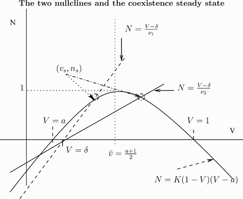
First, we consider . Since , we find that at v=v _s the v-nullcline is above the n-nullcline. This means that , which translates into the condition

For this case we prove stability.

Lemma 2.2

Assume that h(v, n)=v, and χ=0. If then no pattern formation occurs about the coexistence steady state for the system (1) and (2).

Proof

The condition implies that . Hence A<0. In addition, we find B<0, C>0, and D<0 and A<0, B<0, and D<0 imply for all real k. Hence, we cannot expect diffusion-taxis-driven instability about the coexistence steady state.  ▪

In Figure 1 it is noted that v _s should be between a and 1, i.e. a<v _s<1, otherwise n _s is negative. In Lemma 2.2, we considered that and found no pattern. Thus we now consider . First we investigate how many v _s may exist between a and v¯, and then we find conditions for the existence of v _s between a and v¯.

The v values for the coexistence steady state are obtained from

When a<δ, Figure 1 shows that Equation (12) has two real roots. Indeed, for the root less than a, n _s would be negative, which is not biologically relevant. Hence, when a<δ, Equation (12) has one biologically relevant root. In addition, leads to . Therefore, for

the biologically relevant coexistence state exists and its v value is located between .

When a>δ, we may expect two positive roots from Equation (12). However, a simple computation of Equation (12) shows that we cannot have two positive roots. Under assumption (13), the biologically relevant solution of Equation (12) is given by

The discriminant in Equation (14) is zero for

Equations (14) and (15) give a condition for the existence of the coexistence steady state,

which will be used to show that AD−BC>0, whenever v _s exists.

We find A>0 from the condition (13). Additionally, from Equation (9) we find B<0, C>0, and D<0. The stability condition A+D<0 leads to a condition

In Figure 2 we plot the left- and right-hand sides of Equation (16) as a function of v _s.

Figure 2. Plot of the left- and right-hand sides of Equation (16) as function of v _s. The region of A+D<0 is where the dashed line lies above the curve.

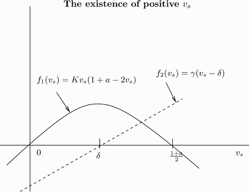
As γ varies from zero to infinity, the intersection of and changes from to . Given a value for v _s, we can always choose γ small enough such that condition (16) is not true. Thus, γ should be greater than a minimum value, γ₀. Here , where v _s is computed in Equation (14). Therefore, for , we have A+D<0.

Thus a biologically relevant v _s is in the interval

We found that Equation (17) holds under assumption (13).

Theorem 2.3

Assume that h(v, n)=v, and χ=0. If a satisfies condition (13), then (i) the coexistence steady state exists (ii) AD−BC>0, (iii) if in addition, there exists such that for each there exists a non-empty interval [k ₁, k ₂] of unstable modes, so we may expect diffusion-driven instability about the coexistence steady state, and (iv) if then is linearly stable.

Proof

• (i) It was shown that condition (13) implies the existence of a unique positive root v _s.

• (ii) When a positive v _s exists, v _s satisfies condition (17). Now we consider the condition for AD−BC>0.

  which holds if . Indeed, this is true by condition (17). Therefore, AD−BC is always positive under the assumption of the existence of a coexistence steady state.

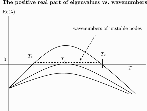
• (iii) M ₁(k ²) and M ₂(k ²) are given by Equations (10) and (11), respectively, with , B=−v _s<0, , and . Hence, A+D<0 guarantees . If , then D<0 gives , hence M ₂(k ²) is always positive. On the other hand, setting , for , we have and M ₂(k ²) can be negative for some k. Setting T=k ², the quadratic equation M ₂(T)=0 may have two roots, T _{1, 2} (see Figure 3). By solving this quadratic equation, it can be shown that for there exist real k ₁ and k ₂. For unstable modes k∈[k ₁, k ₂ with and , we have Re(λ)>0. Hence we may expect diffusion-driven instability about the coexistence steady state (see also 30).

• (iv) If , then M ₂(k ²) is always positive for all k. Hence we cannot expect diffusion-driven instability about the coexistence steady state.

  ▪

Figure 3. Plot of the eigenvalue λ (k ²) as a function of T with T=k ².

Segel and Jackson 30 also considered diffusion-driven instability in a predator–prey interaction. They used and f(v)=1+Kv, and found the wavelength of the instability (see also 26 for general discussion on diffusion-driven instability in a predator–prey interaction).

In particular, for , we apply a perturbation method to approximate two values T _{1, 2}, that is, and . Therefore, for , M ₂(T) is negative.

For example, we consider an interval [0, L] with homogeneous Neumann boundary condition given by Equation (3). If k(n)=nπ/L in [k ₁, k ₂] with positive integer n, then pattern formation occurs. Thus, we can calculate a minimum domain size for pattern formation. Since , we substitute k(n)=nπ/L and rearrange the inequality with respect to L. Then we have

which should hold for some integer n. Therefore, the minimum length for possible instabilities is L*=π/k ₂, and for L<π/k ₂, we cannot expect pattern formation.

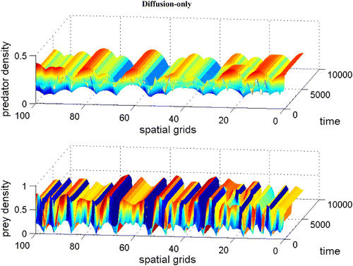
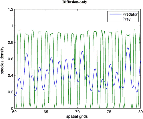
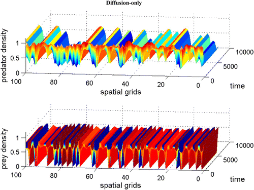
In Figure 4, we show phase portraits of the predator–prey system (1) and (2) without dispersal terms. As γ increases, the coexistence steady state bifurcates from an unstable spiral to a stable spiral. From simulations with various γ, it is noted that an unstable limit cycle occurs for a certain range of γ. When γ is smaller than the lower bound of this range, the coexistence steady state is an unstable spiral. When γ is bigger than the upper bound of the range, the coexistence steady state is a stable spiral with non-empty basin of attraction. Figure 5 shows that the stable coexistence steady state without dispersal terms becomes unstable if diffusion terms are introduced. As a result, patterns are generated. We demonstrate a snapshot of the asymptotic prey and predator distributions in Figure 6. It is noted that high prey density area seems to attract more predators. Moreover, the patch size of prey is seen to be an important factor to attract more predators.

Figure 4. Coexistence steady state is shown to be locally asymptotically stable for system (1) and (2) without dispersal terms and with f(v)=16(1−v)(v−0.5), h(v, n)=v, and δ (n)=0.6+0.1 n. Time step is d t=0.01 and γ=13. Here the coexistence steady state is (v _s, n _s)=(0.695, 0.952). Available in colour online.

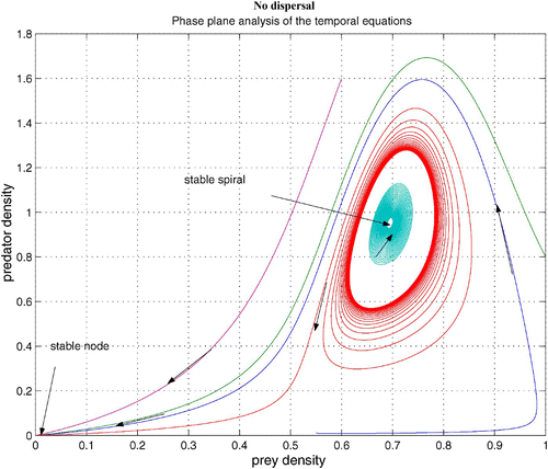
Figure 5. Coexistence steady state is shown to be locally unstable for system (1) and (2) with χ(v)=0.0, f(v)=16(v−0.5)(1−v), h(v, n)=v, and δ (n)=0.6+0.1 n. Spatial grid size is d x=0.25, time step d t=0.01, and γ=14 with 60 time units. The diffusion coefficient ε is 0.01. Here the coexistence steady state is (v _s, n _s)=(0.695, 0.952). Available in colour online.

Figure 6. With the same parameters as in Figure 5, we demonstrate a snapshot of the spatial prey and predator distributions after 60 time units between dimensionless spatial locations 10 and 15. Available in colour online.

2.2. Type I functional response, density-dependent predator death rate, and Allee effect with diffusion and prey-taxis

We now include prey-taxis in the calculations of the previous subsection (Table 1, row 1). We consider the reaction–diffusion–taxis system (1) and (2) for . We consider Allee-type growth for the prey, with 0<a<1 and K=4/(1−a)², a type I functional response, h(v, n)=v, and a density-dependent predator death rate, . We have shown in the previous subsection that for χ=0, pattern formation may occur. In this subsection, we consider how the conditions of pattern formation change if χ is introduced.

Lemma 2.4

Assume a, δ, and ε satisfy instability conditions of Theorem 2.3. Then from Lemma 2.1 we compute

such that the coexistence steady state for system (1) and (2) is linearly stable for each . For there exists an interval [k ₁, k ₂] of unstable modes.

Proof

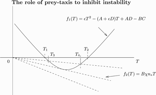
Here M ₁(k ²) from (7) is the same as in the case of diffusion-only (10) so that it is negative for all k. But M ₂(k ²) from (8) is different by the term Bχ n _s. Setting M ₂(k ²)=0 and T=k ², we obtain after rearrangements

Figure 7 shows three typical situations of intersections of the left- hand and the right-hand sides of Equation (18). In the diffusion-only case, we saw that there may be two roots, T ₁ and T ₂, of under the conditions that . Between T ₁<T<T ₂, is negative. In order for M ₂(T) to be negative, the left-hand side of Equation (18) should be less than the right-hand side. In Figure 7, the region T ₃<T<T ₄ where the solid curve is below the dashed line makes M ₂(T) negative. As we can see in Figure 7, T ₃ is always greater than T ₁ and T ₄ smaller than T ₂ for positive χ. As χ gets bigger, the slope of the line of the right-hand side of Equation (18) is steeper so that for there will be no intersection of the curve and the line (see Figure 7). In that case, M ₂(T) is always non-negative, which leads to negative eigenvalues and to stability. In Theorem 2.3, for χ=0, we found a threshold of . For χ≠0, the threshold for pattern formation is

Thus, as χ gets bigger, ε₁ requires smaller value ε for pattern formation.   ▪

Figure 7. Plot of the left- and right-hand sides of Equation (18) as a function of T with T=k ². The solid curve is from the left-hand side of Equation (18) and the dashed lines are from the right-hand side of Equation (18). As χ increases, the number of intersection changes from zero to two. Note that B is negative.

Figure 4 shows that the coexistence steady state for the spatially homogeneous predator–prey system (1) and (2) without dispersal terms is stable. In Figure 5, introducing the diffusion term generates patterns. The numerical simulations confirmed that when we introduce a large prey-taxis term, patterns disappear (not shown here).

2.3. Linear ratio-dependent functional response, constant predator death rate, and logistic growth

In this subsection, we show that pattern formation is impossible when there is a linear ratio functional response and logistic growth along with a constant predator death rate (Table 1, row 2). We consider the linear ratio-dependent functional response, with logistic growth for the prey, f(v)=1−v, and a constant predator death rate, , and ν₀ is a constant parameter. Thus the coexistence steady state is now , which is biologically relevant for . In this case, we obtain

We observe that A<0, D<0, B=0, AD−BC>0, and for all k. Hence, the homogeneous steady state is linearly stable.

Lemma 2.5

Assume f(v)=1−v, and then no pattern formation occurs about the coexistence steady state, for system (1) and (2).

2.4. Hyperbolic ratio-dependent functional response, constant predator death rate, and logistic growth

We now modify the analysis of the previous subsection to include a hyperbolic ratio rather than linear ratio functional response. This allows for the possibility of pattern formation, providing that taxis is sufficiently small (Table 1, row 3). We consider hyperbolic ratio-dependent functional response, with logistic growth for the prey, f(v)=1−v, and a constant predator death rate, , and μ≥0 and d≥0 are constants. Thus the coexistence steady state in this case is

which is biologically relevant for . In this case, we have

We consider conditions that A+D<0 and AD−BC>0. For A<0, it is seen that A+D<0 and AD−BC>0. For A>0, , with

implies that A+D<0.

Lemma 2.6

Assume f(v)=1−v, and χ=0.

• (i)  If no pattern formation occurs about the coexistence steady state, for system (1) and (2).

• (ii)  Assume . There exists such that for each there exists a non-empty interval [k ₁, k ₂ of unstable modes, so we may expect diffusion-driven instability about the coexistence steady state,

• (iii) in case (ii) if then is linearly stable.

Proof

• (i) First, implies A<0. In addition, B<0, C>0, and D<0 result in positive M ₂(k ²) from (11). Hence, we cannot expect diffusion-taxis-driven instability about the coexistence steady state.

• (ii) Second, we consider , which gives A>0. It is also seen that AD−BC>0 and for , A+D<0, which implies that M ₁(k ²) from (10) is negative. However, when ε is less than , then A+ε D is positive. Thus, M ₂(k ²) can be negative. With the same steps in Theorem 2.3, we can find k ₁ and k ₂ with , where

  Consequently for , there exist real k ₁ and k ₂. Furthermore, for k ₁<k<k ₂, we have Re(λ)>0, and we may expect diffusion-driven instability about the coexistence steady state.

• (iii) If , then M ₂(k ²) is positive for all k. Hence, we cannot expect diffusion-driven instability about the coexistence steady state.

  ▪

Alonso et al. 2 also considered a hyperbolic ratio-dependent functional response for pattern formation by using numerical exploration of the parameter space.

Now we can follow the argument of the case including an Allee effect. Thus, the reaction–diffusion system may show diffusion-driven instability depending on parameters μ, d, δ, γ, and ε. Furthermore, the prey-taxis term tends to inhibit the occurrence of dispersal-driven instability (see Lemma 2.1 and Section 2.2 for the full argument).

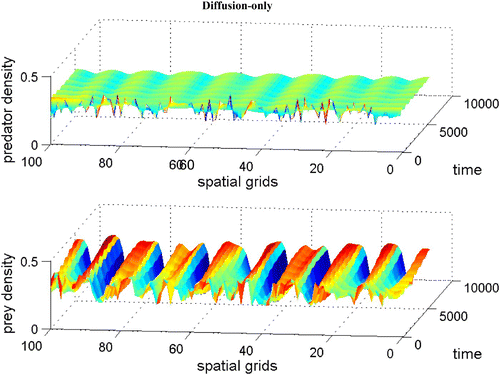
In Figure 8, we show phase portraits of the predator–prey system (1) and (2) with hyperbolic-ratio functional response and without dispersal terms. As γ increases, the coexistence steady state bifurcates from an unstable spiral to a stable spiral. Figure 9 demonstrates that this homogeneous coexistence steady state becomes unstable if diffusion terms are introduced. As a result, patterns are generated. It is shown that when we introduce a large prey-taxis term, patterns eventually disappear (see 17 for figure).

Figure 8. Coexistence steady state is shown to be locally asymptotically stable for system (1) and (2) without dispersal terms and with h(v, n)=0.8 v/(0.05 n+v), f(v)=1−v, and δ (n)=0.76. Time step is d t=0.005, and γ=15. Here the coexistence steady state is (v _s, n _s)=(0.2, 0.211). Available in colour online.

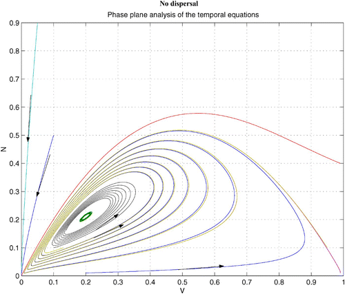
Figure 9. Coexistence steady state is shown to be locally unstable for system (1) and (2) with h(v, n)=0.8 v/(0.05 n+v), f(v)=1−v, and δ (n)=0.76 and with χ(v)=0.0. The diffusion coefficient ε is 0.01. Spatial grid size is d x=0.25, time step dt=0.01, and γ=15. Here the coexistence steady state is (v _s, n _s)=(0.2, 0.211). Available in colour online.

2.5. Type II functional response, density-dependent predator death rate, and logistic growth

Next we consider a hyperbolic functional response and a density-dependent predator death rate from the setting of the previous subsection and show that pattern formation is possible, provided that taxis is sufficiently small (Table 1, row 4). We consider type II functional response, as in 27, a density-dependent predator death rate, , and logistic growth for the prey, f(v)=1−v with α>0, 0<δ<1, and ν>0. The coexistence steady state can be obtained from the root of the following system

By applying the intermediate-value theorem, it is shown that there is at least one point v=v _s in the open interval (0, 1) such that g(v _s)=0. Moreover, since for v _s∈(0, 1), n _s corresponding to v _s is positive as well.

Lemma 2.7

Assume f(v)=1−v, and then there exists at least one coexistence steady state, for the system (1) and (2).

For an homogeneous coexistence steady state , we find

It is noted that B<0, C>0, and D<0. Thus for A<0, we cannot expect spatial pattern because M ₁(k ²)<0 and M ₂(k ²)>0 for all k. The condition for A<0 is rewritten in terms of parameters α, δ, and ν as follows:

Therefore, we can summarize the result.

Lemma 2.8

Assume f(v)=1−v, and . If then no pattern formation occurs about the coexistence steady state, for the system (1) and (2).

This result was also confirmed numerically for selected parameter values (not shown here).

Now we consider the case of A>0, that is,

The condition for

implies (after some computation)

Under condition (19), we set the positive root of A+D expressed above with v*, and then v* is between 0 and . Thus, for v _s in , we have A+D<0. Note: . Recall that v _s is independent of γ, so by controlling γ we can make v* smaller than v _s.

Now we consider AD−BC>0. Because A is positive, we cannot guarantee AD−BC>0. After rearrangement, we find

which is positive if

After some computation, we obtain that

since at , we have A=0. In addition, the continuity of G(v _s) on guarantees that there is at least one root v** in such that G(v**)=0. Therefore, for , we have AD−BC>0.

Theorem 2.9

Assume that f(v)=1−v, and χ=0. {\rm (i)} Then at least one coexistence steady state exists; (ii) there exists a such that for all we have A+D<0 and AD−BC>0; (iii) there exists such that for each there exists a non-empty interval [k ₁, k ₂] of unstable modes, so we may expect diffusion-driven instability about the coexistence steady state; (iv)} if then is linearly stable.

Proof

Property (i) was shown in Lemma 2.7. (ii) It was also shown that for , we have A+D<0 and for , AD−BC>0. Hence, we define , so for , we have A+D<0 and AD−BC>0. (iii) Now M ₂(k ²) is

with , , , and .

If , then D<0 gives , hence M ₂(k ²) is always positive, which results in no diffusion-driven instability for . Therefore, ε should be strictly less than 1. Indeed, setting , then for , we have and M ₂(k ²) can be negative for some k.

By setting T=k ², we have a quadratic form of M ₂(T), that is, . Solving this quadratic form gives that there are two positive ε, say ε₁ and ε₂ with , such that for , M ₂(T) has two positive roots, say T ₁ and T ₂ with T ₁<T ₂. Therefore, M ₂(T) is negative for k∈(k ₁, k ₂) with and . For unstable modes k∈[k ₁, k ₂], we have Re(λ)>0. Hence we may expect diffusion-driven instability about a coexistence steady state .

(iv) If , then M ₂(k ²) is always positive for all k. Hence, we cannot expect diffusion-driven instability about the coexistence steady state.   ▪

For χ≠0, we obtain a similar result as in Section 2.2.

Lemma 2.10

Assume that instability conditions of Theorem 2.9 are satisfied. Then we define

such that a coexistence steady state for system (1) and (2) is linearly stable for each . For there may exist an interval [k ₁, k ₂] of unstable modes.

Proof

See Lemma 2.1   ▪

Figure 10 demonstrates that the stable coexistence steady state without dispersal terms becomes unstable when diffusion terms are introduced (Theorem 2.9). As a result, patterns are generated. It is shown that when we introduce a large prey-taxis term, patterns are disappearing (Lemma 2.10 and see 17 for figure).

Figure 10. Coexistence steady state is shown to be asymptotically unstable for system (1) and (2) with χ=0, f(v)=1−v, h(v, n)=v(α+1)/(α+v), and δ(n)=δ+ν n with α=0.2, δ=0.6, γ=1.2, and ν=0.4. The diffusion coefficient ε is 0.01. Spatial grid size d x=0.25 and time step d t=0.01 with 60 time units. Here the coexistence steady state is (v _s, n _s)=(0.296, 0.291). Available in colour online.

2.6. Type II functional response, constant predator death rate, and logistic growth

We now modify the analysis of the previous subsection to include a constant rather than density-dependent predator death rate. This does not allow for the possibility of pattern formation (Table 1, row 5). We consider type II functional response, as in 27, a constant predator death rate, , and logistic growth for the prey, f(v)=1−v. Thus the coexistence steady state is

which is biologically relevant for . In this case,

and consequently,

for all k. Thus the homogeneous steady state is linearly stable.

It is noted that type II functional response does not play any role in pattern formation versus type I. In a numerical solution (not shown) with χ=6.5 and a randomly chosen initial distribution, we observe that the solution converges to the coexistence equilibrium .

2.7. Type I functional response, density-dependent predator death rate, and logistic growth

We now modify the analysis of Section 2.5 to include a type I rather than type II functional response. This also does not allow for the possibility of pattern formation (Table 1, row 6). We include competition in the predator death rate, so the predator death rate is . In addition, we consider type I functional response, h(v, n)=v, and logistic growth for the prey, f(v)=1−v. Thus the coexistence steady state is , which is biologically relevant for . In this case, we obtain

We find A<0 and D<0 for biologically relevant δ, which result in A+D<0. Moreover, B<0 and C>0 give rise to AD−BC>0. In addition, A<0, D<0, B<0, and AD−BC>0 give for all k. Hence, we note that M ₂(k ²)>0 for all k, hence the homogeneous steady state is linearly stable.

This result was also confirmed numerically for selected parameter values (not shown here).

3. Global stability

In the previous section, we showed that without both the Allee effect and the density-dependent predator death rate, diffusion, and prey-taxis do not change the local stability of the coexistence steady state. We choose one of the cases without pattern formation to study the global stability of . We consider logistic growth for the prey, f(v)=1−v, a type I functional response, h(v, n)=v, a density-dependent predator death rate, , and a non-constant prey sensitivity, χ (v)=b/v, for the spatially homogeneous case of system (1) and (2) on an interval Ω=[0, L] with homogeneous Neumann boundary conditions (3). The following Lyapunov function,

has been used to show the global stability of 5. We will show that is a Lyapunov functional for the spatially dependent problem (1) and (2) in this case.

Theorem 3.1

Let f(v)=1−v, h(v, n)=v, and with boundary condition (3). We assume that then the functional V(v, n) defined in Equation (20) is a strong Lyapunov function for system (1) and (2). The sets are positively invariant and is globally asymptotically stable.

Proof

Setting for L large enough, then we claim that the sets N _L are positive invariant. When , becomes zero due to [Vtilde]=0. For v>v _s, the first term of Equation (20) is positive. Similarly, the second term of (20) is positive. Therefore, [Vtilde] is positive in N _L . Hence, the functional, V(v, n), is bounded below by zero. Moreover, the definition of the Lyapunov functional,

leads to and . Since

V(v, n) is continuously differentiable for v, n>0. The next step is showing that for (v, n)∈N _L , d V/d t is negative definite for a certain parameter space.

We arrange the right-hand side of this equation into two parts; one including the local dynamics and the other including the dispersal terms. First we look at the local dynamics

(see also 5 for the case of a constant death rate of the predator). Here (v−v _s) and have the opposite sign with f(v)=1−v so that is negative. Similarly, (n−n _s) and have the opposite sign due to . Therefore, is negative unless . We now take into account the dispersal term of (21) by using integration by parts with zero flux boundary condition

where

Thus, the matrix A is symmetric. Hence, if A is positive definite, all eigenvalues of the matrix A are positive. Here tr is positive. Thus a positive determinant

guarantees two positive eigenvalues for the matrix A. As a result, for (v, n)∈N _L . With the specific example of χ(v)=b/v, we have the condition for positive eigenvalues that . For the special case of χ(v)=0, i.e. diffusion-only case, the matrix A is always positive definite for N _L . Therefore, the functional V(v, n) is shown to be a Lyapunov functional under the condition specified above. Thus, V(v, n)→0 as t→∞, so v→v _s and n→n _s. Therefore, the homogeneous steady state is globally asymptotically stable.   ▪

4. Conclusion

In this paper, we considered pattern formation for a predator–prey taxis model of reaction–diffusion–advection type given by (1) and (2). We considered various reaction terms: for the predator term they include type I and type II functional responses as well as ratio-dependent functional responses. We considered constant and density-dependent death rate of the predator and logistic growth or an Allee-type growth for the prey.

In summary, the following functional forms support spatial pattern formation:

• (i) a density-dependent death rate, e.g. , and an Allee effect, e.g. , and a type I functional response, e.g. h(v, n)=v:

  • patterns form with no prey-taxis (Section 2.1),

  • patterns persist with small prey-taxis but disappears for large prey-taxis (Section 2.2),

  • patterns disappear when Allee dynamics are replaced by logistic dynamics (Section 2.7),

• (ii) a hyperbolic ratio-dependent functional response, e.g. and logistic growth, e.g. f(v)=1−v:

  • patterns form with no prey-taxis (Section 2.4),

  • patterns persist with small prey-taxis but disappears for large prey-taxis (Section 2.4),

  • patterns disappear if a hyperbolic functional response is replaced by a linear functional response (Section 2.3);

• (iii) a density-dependent death rate, e.g. , and a type II functional response, e.g. .

  • patterns form with no prey-taxis (Section 2.5),

  • patterns persist with small prey-taxis but disappears for large prey-taxis (Section 2.5),

  • patterns disappear if a density-dependent predator death rate is replaced by a constant predator death rate (Section 2.6).

The significance of this research is as follows; contrary to a diffusion process that may give rise to pattern formation, prey-taxis tends to stabilize predator–prey interactions (Theorem 2.3). In the long run, prey-taxis tends to transform heterogeneous environments into homogeneous environments, which gives an opposite result to the chemotaxis case. Under strong chemotactic sensitivity, amoebae tend to aggregate 29. Hence the role of taxis may be strongly related to the local population dynamics of the species.

In this paper, prey-taxis is shown to tend to reduce the likelihood of pattern formation in spatial predator–prey systems, but other kinds of taxis may have the opposite effect on pattern formation. For example, we may investigate prey defences. Prey tend to adjust their relative position to the predator to reduce predation risk 10 24 37 38. We may apply the concept of prey-taxis to prey escape response to predator density. It may refer to predator-taxis. For instance, crayfish (prey) exhibit different activities depending on the presence of a predator (bass). An increased predation risk restricts crayfish foraging and increases anti-predator behaviour such as shelter seeking 8 11. Another interesting taxis is that predators may attract their prey to come nearby 31. In this case, prey move towards predators. As a conjecture, from Equation (8), we may predict that positive predator-taxis (away from predators) tends to generate pattern formation but negative predator-taxis (towards predators) tends to inhibit pattern formation. However, the detailed argument is left for future work.

Acknowledgements

We thank G. de Vries, C. Cosner, and C.J. Bampfylde for helpful discussion and comments on the manuscript. We appreciate two anonymous reviewers for helpful comments and suggestions. We would also like to thank all the members of the Lewis lab for encouragement and feedback, which have improved this research. JML was supported by a University of Alberta Studentship and by an NSERC collaborative Research Opportunity Grant. TH was supported by NSERC. ML was supported by NSERC and a Canada Research Chair.

References

- Allen , M. B. and Eli , M. B. 1998 . Numerical Analysis for Applied Science , New York : Wiley-Interscience .
- Alonso , D. , Bartemeus , F. and Catalan , J. 2002 . Mutual interference between predators can give rise to Turing spatial patterns . Ecology , 83 : 28 – 34 .
- Arditi , R. , Tyutyunov , Y. , Morgulis , A. and Govorukhin , V. 2001 . Directed movement of predators and the emergence of density-dependence in predator-prey models . Theoret. Population Biol. , 59 : 207 – 221 .
- Biktashev , V. N. , Brindley , J. , Holden , A. V. and Tsyganov , M. A. 2004 . Pursuit-evasion predator-prey waves in two spatial dimensions . Chaos , 91 : 218102
- Britton , N. F. 1986 . Reaction-Diffusion Equations and Their Applications to Biology , London : Academic Press .
- Chakraborty , A. , Singh , M. , Lucy , D. and Ridland , P. 2007 . Predator-prey model with prey-taxis and diffusion . Math. Comput. Model. , 46 : 482 – 498 .
- Dolak , Y. and Hillen , T. 2003 . Cattaneo models for chemosensitive movement numerical solution and pattern formation . J. Math. Biol. , 46 : 153 – 170 .
- Garvey , J. E. , Stein , R. A. and Thomas , H. M. 1994 . Assessing how fish predation and interspecific prey competition influence a crayfish assemblage . Ecology , 75 ( 2 ) : 532 – 547 .
- Grunbaum , D. 1998 . Using spatially explicit models to characterize foraging performance in heterogeneous landscapes . Am. Nat. , 151 : 97 – 115 .
- Hamilton , W. D. 1971 . Geometry for the selfish herd . J. Theor. Biol. , 31 : 295 – 311 .
- Hill , A. M. and Lodge , D. M. 1999 . Replacement of resident crayfishes by an exotic crayfish: the roles of competition and predation . Ecol. Appl. , 9 ( 2 ) : 678 – 690 .
- Hillen , T. and Painter , K. 2001 . Global existence for a parabolic chemotaxis model with prevention of overcrowding . Adv. Appl. Math. , 26 ( 4 ) : 280 – 301 .
- Jorné , J. 1974 . The effects of ionic migration on oscillations and pattern formation in chemical systems . J. Theor. Biol. , 43 : 375 – 380 .
- Kareiva , P. and Odell , G. 1987 . Swarms of predators exhibit ‘preytaxis’ if individual predators use arearestricted search . Am. Nat. , 130 : 233 – 270 .
- Kolokolnikov , T. , Erneux , T. and Wei , J. 2006 . Mesa-type patterns in the one-dimensional brusselator and their stability . Phys. D , 214 : 63 – 77 .
- Kurganov , A. and Tadmor , E. 2000 . New high resolution central schemes for nonlinear conservation laws and convection-diffusion equations . J. Comput. Phys. , 160 : 214 – 282 .
- Lee , J. 2006 . Prey-taxis and its applications , Edmonton, , AB, Canada : University of Alberta . Ph.D. thesis
- Lee , J. , Hillen , T. and Lewis , M. A. 2007 . Prey-taxis equations: continuous travelling waves for pest control . in preparation
- LeVeque , R. J. 2002 . Finite Volume Methods for Hyperbolic Problems , Cambridge : Cambridge University Press .
- Lewis , M. A. 1994 . Spatial coupling of plant and herbivore dynamics: the contribution of herbivore dispersal to transient and persistent ‘waves’ of damage . Theor. Population Biol. , 45 : 277 – 312 .
- Losey , J. E. and Denno , R. F. 1998c . The escape response of pen aphids to foliar-foraging predators: factors affecting dropping behaviour . Eco. Entom. , 23 : 53 – 61 .
- Malchow , H. 1995 . Flow-and locomotion-induced pattern formation in nonlinear population dynamics . Ecol. Model. , 82 : 257 – 264 .
- Malchow , H. 2000 . Motional instability in prey-predator system . J. Theor. Biol. , 204 : 639 – 647 .
- Morton , T. L. , Haefner , J. , Nugala , V. , Decino , R. D. and Mendes , L. 1994 . The selfish herd revisited: do simple movement rules reduce relative predation risk . J. Theor. Biol. , 167 : 73 – 79 .
- Murray , J. D. 1989 . Mathematical Biology , New York : Springer Verlag .
- Okubo , A. and Levin , S. A. 2000 . Diffusion and Ecological Problems: New Perspectives , 2 , New York : Springer Verlag .
- Owen , M. R. and Lewis , M. A. 2001 . How predation can slow, stop or reverse a prey invasion . Bull. Math. Biol. , 63 : 655 – 684 .
- Rovinsky , A. B. and Menzinger , M. 1992 . Chemical instability induced by a differential flow . Phys. Rev. Lett. , 69 : 1193 – 1196 .
- Segel , L. A. 1980 . Mathematical Models in Molecular and Cellular Biology , Cambridge : Cambridge University Press .
- Segel , L. A. and Jackson , J. 1972 . Dissipative structure: an explanation and an ecological example . J. Theor. Biol. , 37 : 545 – 559 .
- Shi , W. and Zusman , D. R. 1993 . Fatal attraction . Nat. Sci. , 366 : 414 – 415 . Correspondence
- Strikwerda , J. C. 1989 . Finite Difference Schemes and Partial Differential Equations , CA : Wadsworth, Inc .
- Tsyganov , M. A. , Brindley , J. , Holden , A. V. and Biktashev , V. N. 2003 . Quasisoliton interaction of pursuitevasion waves in a predator-prey system . Phys. Rev. Lett. , 91 : 218102
- Turchin , P. 2003 . Complex Population Dynamics , Princeton and Oxford : Princeton University Press .
- Tyson , R. , Lubkin , S. R. and Murray , J. D. 1999 . Model and analysis of chemotactic bacterial patterns in a liquid medium . J. Math. Biol. , 38 : 359 – 375 .
- Tyson , R. , Stern , L. G. and LeVeque , R. J. 2000 . Fractional step methods applied to a chemotaxis model . J. Math. Biol. , 41 : 455 – 475 .
- Viscido , S. V. and Wethey , D. S. 2002 . Quantitative analysis of fiddler crab flock movement: evidence for ‘selfish herd’ behaviour . Anim. Behav. , 63 : 735 – 741 .
- Viscido , S. V. , Miller , M. and Wethey , D. S. 2001 . The response of a selfish herd to an attack from outside the group perimeter . J. Theor. Biol. , 208 : 315 – 328 .